A high performance acoustic microscope - technical aspects and selected applications

A HIGH PERFORMANCE ACOUSTIC MICROSCOPE - TECHNICAL ASPECTS AND SELECTED APPLICATIONS

Abdullah Atalar+ and Martin Hoppe*

+Electrical and Electronics Engineering Department Middle East Technical University

ABSTRACT

06531 Ankara, Turkey

*Ernst Leitz Wetzlar GmbH P.Box 2020

D-6330 Wetzlar, FRG

Technical aspects of a scanning acoustic microscope with broad frequency coverage (50 .•• 2000 MHz) are described. Images demonstrating the capabilities of the microscope are shown.

INTRODUCTION

The scanning acoustic microscope is finding applications as a powerful scientific instrument for imaging and

characterization of materials (Ash, 1980; IEEE Trans. Sonics Ultrasonics SU-32, 1985). A few commercial instruments have

shown up recently at the marketplace. In this paper, we decribe the scanning acoustic microscope (ELSAM)* developed at Ernst Leitz Wetzlar GmbH, West Germany (Hoppe et al., 1983; Hoppe et al., 1985) following the guidelines of Stanford

microscope (Lemons, 1974; Quate et al., 1979; Jipson et al., 1978) .

ELSAM is an acoustic microscope combined with an optical microscope capable of generating visual or hard-copy acoustic images. Use of microprocessors released the user from routine adjustments of the complicated system, and also the hardware and wiring is simplified to result in a reliable system. In this paper, we also present some selected acoustic images obtained with ELSAM which show the capabilities of the scanning acoustic microscope.

USER _.... HIGH FREQUENCY

a.

~ ~

TERMI NAL _ELECTRONICS

+

~

1

t

POWER SI GNAL PROC.ESSI NG

SCA N 2- CONTROL SUPPLY

ELECTRONICS

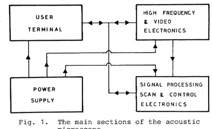
Fig. 1. The main sections of the acoustic microscope

GENERAL DESIGN FEATURES

The wavelength of the acoustic waves used in imaging is determined by the frequency of operation. To serve both high resolution and high penetration depth applications, an acoustic microscope with broad frequency coverage is necessary. The 50 - 2000 MHz frequency band is selected to be the operation range. For ease of operation and for compatibility with many obje€ts the coupling liquid is selected to be water. To get both optical and acoustical information from the same area of the object, a reflected-light microscope is combined with the acoustic microscope. The mechanical accuracy of conversion between the two micorscopes is such that the obtained images are centered to within a few micrometers of each other.

The main'sections of the acoustic microscope are its mechanical parts, its electrical parts and its acoustic part as depicted in Fig. 1 in block diagram form. The critical mechanical parts include the X-Y scan mechanism, the Z adjust-ment mechanics, the object leveling apparatus. The X-Y scan mechanism is able to generate a 1 mm by 0.8 mm raster scan with less than 0.3 micrometer deviation in the Z direction. It is a electromechanical scan utilizing electromagnets and long leaf springs. Z adjustment can be done either manually or remotely by an electrical motor. The object leveling

apparatus is coupled to the object stage to adjust the object surface parallel to the X-Y scan plane.

The user terminal is a small terminal designed around an 8-bit microprocessor to, take commands from the user and send it to the other parts of the microscope for the selected operating mode to act as a controller for the acoustic

microscope system. It is also used to inform the user on the modes of the microscope. The terminal has a dedicated keyboard and a joy-stick through which all the commands and adjustments are easily entered, and a 40 x 2 character plasma display on which all the relevant information is shown. Through the keyboard the user can select the various display and signal processing modes, change the magnification or the operation frequency.

HIGH FREQUENCY ELECTRONICS

The high frequency electronics operates in the pulse-echo mode. It receives commands from the user terminal and sets its operating point accordingly. The 50 - 2000 MHz frequency band is divided between two units. A block diagram of the high frequency electronics operating at 0.8 GHz to 2.0 GHz is shown in Fig. 2. It is basically composed of transmitter oscillators, pulse generating circuits and a superheterodyne receiver. The transmitted signal is generated by varactor tuned oscillators whose frequency can be

controlled by a voltage applied from a D/A converter driven by a computer. This signal is pulsed by a solidstate switch to generate 10 nsec pulses. The switch is driven by a pulse drive electronics again controlled by the computer. The pulsed rf signal is amplified to a level of 1 W. The signal is fed to one of the arms of a double throw switch. The

COMPUTER INTERFACE VIDEO OUT OFFSET ADJ

8

Fig. 2. The high frequency electronics for the 800 - 2000 MHz range IMPULSE GENERATOR COMPUTER Hi PASS FILTER POWER DIVIDER TO VIDEO AMP MATCH. NETW. POWER LIMITER

Fig. 3. The high frequency electronics for the 50 - 800 MHz range

common arm of the switch is connected to the acoustic lens element. The second arm of the switch goes to a wide-band preamplifier. The pulse drive interface driving this switch is adjusted such that the first arm is connected to the common arm only when the first switch is on and the second arm is connected to common arm at a time slightly after the trans-mitter pulse is applied to the lens element. The output of the preamplifier is fed to a wide band mixer. The local oscillator is also pulsed to keep the IF amplifiers away from the

saturation caused by the spurious reflections. The local oscillator is turned on only during the time the object pulse may appear. The necessary pulse is created by the pulse drive electronics using computer controlled digital delay techniques. The frequency of the local oscillator is corrected by the

microprocessor to maximize the output voltage each time a new frequency is selected. The two intermediate frequency

(IF)amplifiers in cascade provide the necessary gain. There is another switch between the two IF amplifiers to further reduce the undesired pulses. The gain of the IF amplifier is adjustable by the computer to the desired level. Finally, the output of the IF amplifier is detected by a detector diode to generate the video signal which is proportional to the

amplitude of the received acoustic signal. The computer

responsible for the whole high frequency electronics is built around an 8-bitsingle-chip microprocessor.

A block diagram of the high frequency electronics suit-able for the 50 - 800 MHz range is depicted in Fig. 3.

A. ,1 nanosecond duration base-band pulse is used to excite the transducer. This pulse is fed to the transducer through a power divider. The output of the power divider is connected to a limiter to protect the input of the receiver amplifier. After amplification a mixer is used as a switch to gate out the unwanted parts of the incoming pulse train. After the time-gating operation further amplification is performed. High pass filters are placed in the receiving chain to get rid of switching spikes caused by the time gating operation. The amplitude detection of the amplifier output provides the necessary video signal for further processing.

The basic functions of video electronics are to shift the DC level of the video signal and to change the video gain. Those variables can be adjusted by the user with the joy-stick on the user terminal. The signal. processing electronics is responsible to make some simple signal processing functions like inverting the video signal to get reverse video images, or differentiating it to get emphasized edges in the images. The video gain can be adjusted either automatically or

manually. The circuitry is controlled by the third computer of the acoustic microscope system. The output of this section is fed to either a high persistence cathode-ray-tube (CRT) fo.r display or to a high resolution CRT for photographing purposes.

SCAN AND CONTROL ELECTRONICS

The s.can electronics takes care o.f various display modes by generating. the appropriate scan drive signals for mechanical scan parts. It is possible t.o change the· magnifi-cation just by changing the drive amplitude for X and Y scans ..

A complete raster scan may contain 64, 128, 512 or 1024

horizontal lines and will be completed within a time interval which varies between 1 to 17 seconds depending on the scan magnitude and on the number of lines selected. If desired, the Y scan can be stopped to investigate just a single scan line. The video signal can be applied to Z input of CRT or to the Y input or a combination of both to get three-dimensional-like display forms. All the functions of the scan electronics are directed by the third computer and they are selected by the user at the user terminal.

The control electronics performs the miscellaneous functions like controlling the temperature of liquid medium, changing the object to lens distance all under computer command and under user instructions.

ACOUSTIC OBJECTIVE

The heart of the acoustic microscope system is its acoustic objective. It converts the electrical signals fed to it into ultrasonic signals, focusses them to a diffraction limited spot and converts the reflected acoustic signals back to the electrical form. The lenses are manufactured from single-crystal sapphire material. A spherical lens cavity is ground on one side of the sapphire with mechanical means. A ZnO thin film tranducer is deposited on the flat side of the crystal. The transducer generates planar acoustic wave fronts when used as transmitter, and as a receiver it is sensitive to the shape of the wave fronts impinging on it. The lens cavity is coated with a quarter-wavelength thick glass anti-reflection layer to reduce the anti-reflection loss. The two-way conversion loss of tranducers is typically 10 dB. The lens units are housed in small metallic tubes with the high frequency connector on one end and the lens on the other. Matching networks are included within the lens housing.

Due to bandwidth limitations the whole frequency range can not be taken care of with a single acoustic objective. Instead, the 0.8 to 2.0 GHz range is divided between two objectives: One centered at 1 GHz and the other at 1.7 GHz. The lower frequency 50 to 800 MHz range is covered by objectives operating at the following center frequencies: 100 MHz, 200 MHz and 400 MHz. A 50 MHz objective is in

preparation. All the objectives have the associated matching networks to give the necessary bandwidth. The acbustic

objectives differ not only in frequency but also in radius of lens cavity. At high frequencies the loss in the liquid medium is very high. In this case lenses with a cavity radius of 40 micrometers are used. On the other hand, at low frequencies the liquid losses drop very rapidly making large radius lenses feasible. At the low frequency end, 2000 mi-crometer radius lenses are used to increase the working distance and to make higher imaging depth possible. Working with large radius lenses is easy both from mechanical and from electrical points of view. Mechanically there is a big playroom and electrically the various internal reflection pulses are well separated from each other. On the other hand, for a 40 micrometer radius lens there is only 60 nsec sepa-ration between the first internal reflection pulse and the object pulse. Additionally the size of the object pulse is

Fig. 4. The microscope in acoustic imaging mode

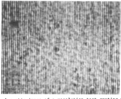
Fig. 5. Acoustic image of a resolution test grating with a period of 0.83 ~m, taken at f

=

(corre-sponding wavelength in water ~ 1 ~m).

60 dB below the spurious pulse. Any reflection in electron-ics or in cables will manifest itself as interference of object pulse with a reference. The high frequ~ncy electronics

described above is capable of separating the small object pulse from its large and close neighboring spurious pulses to generate interference free images.

The objectives of varying lens radii have varying time delays. The object pulse will not appear at the same place for the different objectives. Hence, the delays of time

gating pulses as generated by the pulse drive circuitry should be different. This time delay adjustment is made automatically for every acoustic objective by the microprocessors.

IMAGES

Fig. 4 depicts the ELSAM in its acoustic imaging mode. Referring to the figure, the housing close to the center contains the scanning mechanism for x-y movement of the acoustic objective and the stage with micrometer spindles. The acoustic objective cannot be seen in this picture. The light microscope, here out of its operating position, is on the right side of the scanner housing. At the rear right is a long-persistence CRT screen for real-time display of the acoustic slow scan image. On the table below is the user terminal with joystick and function display. A photomicro-graphic unit with a high-resolution CRT screen is located in front of the user terminal.

Figs. 5 - 7 demonstrate the high resolution and depth penetration ability of the acoustic microscope. All images were obtained from ELSAM high resolution CRT screen with a 35-mm camera attached to it. Brighter pixels represent higher levels of received signal from the corresponding object point. Darker pixels do not necessarily indicate that the acoustic energy at the object is absorbed; the reduction of the signal may be as a result of a cancellation at the phase sensitive transducer (Quate et al., 1979.)

OUTLOOK

The scanning acoustic microscope is a microscope capable of subsurface imaging with a resolution equalling a good optical microscope. Optically opaque materials or layers, which are unsuitable for the optical microscope, become the objects of the acoustic microscope. The acoustic microscope can be used with almost all objects and nondestructively. It is sensitive to a change in density or stiffness of the material. Voids within the body of the materials or

delaminations in thin film structures are easily detected due to very high acoustic impedance change at the interface. The scanning acoustic microscope has found applications in such diverse fields as materials science, thin film technology, geology, biology and new fields are emerging as the appli-cation research continues.

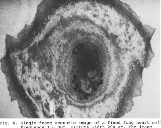
Fig. 6. Single-frame acoustic image of a fixed frog heart cell. Frequency 1.6 GHz, picture width 200 ~m. The image

shows fringes due tocelltopography. Structural

details in the 1 ~m-range are visible (stress fibers).

tal

(b)

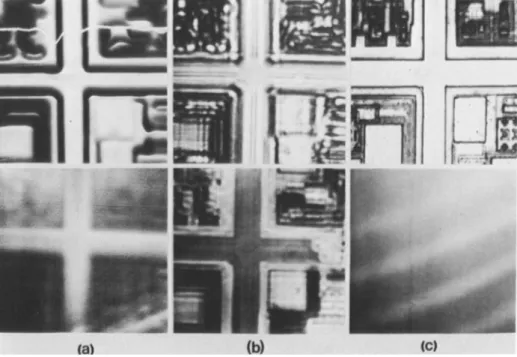
Fig. 7. Depth penetration ability of the acoustic microscope at different frequencies: (a) 100 MHz, (b) 200 MHz,

(c) 400 MHz; width of images 0.8 mm.

Upper row shows surface images of an integrated circuit (IC) .

Bottom row shows pictures of the same area, but imaged through a 250 ~m thick sheet of mica

(water - coupled to the IC surface). At 400 MHz, the mica is not penetrated (c).

Enhanced resolution vs. higher frequencies is clearly visible, too.

REFERENCES

Ash, E.A., 1980, "Scanned Image Microscopy", Academic, London.

IEEE Trans. Sonics Ultrasonics, 1985, SU-32.

Hoppe, M., Atalar, A., Patzelt, W.J. and Thaer, A., 1983, "LEITZ-Akustomikroskop ELSAM: Anwendungen in der Materialuntersuchung - erste Ergebnisse",

Leitz - Mitt. Wiss. u. Techn., VIII: 125 Hoppe, M. and Bereiter-Hahn, J., "Applications of

Scanning Acoustic Microscopy - Survey and New Aspects", 1985, IEEE Trans. Son.Ultrason., 32: 289.

Lemons, R. and Quate, C.F., 1974, Appl. Phys. Lett. ,24: 163.

Quate, C.F., Atalar, A. and Wickramasinghe, K.K., 1979,

Proc. IEEE 67: 1092.

Jipson, V. and Quate, C.F., 1978, Appl. Phys. Lett. ,32: 789.