a thesis
submitted to the department of computer engineering
and the graduate school of engineering and science
of bilkent university
in partial fulfillment of the requirements
for the degree of
master of science
By
Cansın Yıldız
Assist. Prof. Dr. Tolga C¸ apın (Advisor)
I certify that I have read this thesis and that in my opinion it is fully adequate, in scope and in quality, as a thesis for the degree of Master of Science.
Prof. Dr. B¨ulent ¨Ozg¨u¸c
I certify that I have read this thesis and that in my opinion it is fully adequate, in scope and in quality, as a thesis for the degree of Master of Science.
Assoc. Prof. Dr. Veysi ˙I¸sler
Approved for the Graduate School of Engineering and Science:
Prof. Dr. Levent Onural Director of the Graduate School
Supervisor: Assist. Prof. Dr. Tolga C¸ apın June, 2012
This thesis proposes a method that resembles a natural pen and paper interface to create curve based 3D sketches. The system is particularly useful for rep-resenting initial 3D design ideas without much effort. Users interact with the system by the help of a pressure sensitive pen tablet, and a camera. The input strokes of the users are projected onto a drawing plane, which serves as a paper that they can place anywhere in the 3D scene. The resulting 3D sketch is visu-alized emphasizing depth perception by implementing several monocular depth cues, including motion parallax performed by tracking user’s head position. Our evaluation involving several naive users suggest that the system is suitable for a broad range of users to easily express their ideas in 3D. We further analyze the system with the help of an architect to demonstrate the expressive capabilities of the system that a professional can benefit.
Keywords: Human Computer Interaction, Sketch Based Modeling, Sketching,
Depth Perception, Depth Cues, Face Tracking, Pen Tablet. iii
TABLET TABANLI 3 BOYUTLU C
¸ ˙IZ˙IM S˙ISTEM˙I
Cansın Yıldız
Bilgisayar M¨uhendisli˘gi, Y¨uksek Lisans Tez Y¨oneticisi: Yrd. Do¸c. Dr. Tolga C¸ apın
Haziran, 2012
Bu tez normal ka˘gıt ve kalem kullanıyormu¸scasına kavisli ¸sekiller ¸cizmeyi sa˘glayan bir y¨ontem ¨one s¨urmektedir. Sistem ¨ozellikle akla gelen 3 boyutlu fikirleri zaman kaybetmeden dijital ortama aktarabilmek i¸cin kullanı¸slıdır. Kullanıcılar, basınca duyarlı grafik-tablet ve kamera yardımıyla sistemle etkile¸sim haline ge¸cerler. Kul-lanıcıların tablet y¨uzeyine dokunu¸sları bir ¸cizim d¨uzlemine aktarılır ve bu d¨uzlem 3 boyutlu sahnede herhangi bir yere yerle¸stirilebilir. Sistem tek g¨ozle ilgili derin-lik ipu¸clarını ve kullanıcının kafa pozisyonunundan elde etti˘gi hareket paralaksını uygulayarak 3 boyutlu ¸cizime derinlik anlamı katar. Sistemin kullanı¸slılı˘gı ¨uzerine ¸cizim tecr¨ubesi olmayan kullanıcılarla yaptı˘gımız testler, bu sistemin geni¸s bir kitlenin 3 boyutlu ¸cizimler yapabilmesi i¸cin uygun oldu˘gunu g¨ostermektedir. Ayrıca profesyonel bir ki¸sinin sistemin daha anlamlı ve etkili ¨ozelliklerinden nasıl yararlanabilece˘gini g¨ostermek i¸cin bir mimarın katılımıyla daha ileri seviyede bir inceleme de yaptık.
Anahtar s¨ozc¨ukler : ˙Insan Bilgisayar Etkile¸simi, C¸ izim Tabanlı Modelleme, C¸ izim, Derinlik Algısı, Derinlik ˙Ipu¸cları, Y¨uz ˙Izleme, Grafik Tablet.
First and foremost, I have been indebted in the preparation of this thesis to my supervisor, Assist. Prof. Dr. Tolga C¸ apın of Bilkent University, whose patience and kindness, as well as his academic experience, have been invaluable to me. I also want to express my gratitude to Prof. Dr. B¨ulent ¨Ozg¨u¸c and Assoc. Prof. Dr. Veysi ˙I¸sler for showing keen interest to the subject matter.
I am extremely grateful to Mr. Abd¨ulkadir Toyran for demonstrating the capabilities of my system by creating the most pleasing 3D sketches. Similarly, Mr. G¨okhan T¨uys¨uz helped me a great deal with proof-reading this thesis. My friends and colleagues who participated in the user evaluation of the system have been most helpful as well. The informal support and encouragement of many of them was indispensable.
I especially want to thank my beloved G¨ul¸sah for her patience and extreme support throughout all those years. She was always there for me when I was in need.
Most important of all, my parents, Nermin and Emin Yıldız, have been a constant source of emotional and moral support during my postgraduate years, and this thesis would certainly not have existed without them.
Contents vi
List of Figures viii
List of Tables xiii
1 Introduction 1
2 Background & Related Work 4
2.1 Sketch Based Interfaces for Modeling . . . 4
2.1.1 Sketch Acquisition . . . 5 2.1.2 Sketch Filtering . . . 7 2.1.3 Sketch Interpretation . . . 9 2.2 Depth Perception . . . 14 2.2.1 Oculomotor Cues . . . 14 2.2.2 Monocular Cues . . . 15 2.2.3 Binocular Cues . . . 18 vi
2.3.2 Continuously Adaptive Mean Shift . . . 25 3 The System 30 3.1 Overview . . . 31 3.2 Sketching Pipeline . . . 33 3.2.1 Sketch Acquisition . . . 33 3.2.2 Sketch Filtering . . . 33 3.2.3 Sketch Interpretation . . . 36 3.3 Visualization Pipeline . . . 43
3.3.1 Pictorial Depth Effects . . . 44
3.3.2 Face Tracking for Kinetic Depth Effect . . . 47
4 Evaluation, Results & Discussion 54 4.1 Expert Evaluation . . . 54 4.2 User Evaluation . . . 56 4.2.1 Effectiveness . . . 56 4.2.2 Efficiency . . . 59 4.2.3 Satisfaction . . . 60 5 Conclusion 62
Bibliography 64
A Data 71
A.1 Sample Usage Data Collected for
Objective User Evaluation . . . 71 A.2 Survey Questions for Subjective User
Evaluation . . . 73 A.3 Sample Sketch Data that Represents a Scene . . . 74
2.1 The SBIM pipeline: First the input sketch is acquired and filtered. Then, the resulting smoothed input is interpreted as a 3D operation. 5 2.2 SBIM systems acquire input from pen-based devices such as a pen
tablet (a) or tablet display (b). (Wacom Bamboo and Cintiq, re-spectively.) . . . 5 2.3 (a) A stroke is performed by the user, (b) captures as a sequence
of discrete points by pen device; (c) an image-based representation can also be used to represent the input. Reprinted from [42]. . . . 6 2.4 Filtering operations: (a) smooth uniform resampling; (b) coarse
polyline approximation; (c) fit to a spline curve. Reprinted from [42]. . . 8 2.5 Over-sketching: (a) initial curve; (b) oversketch gesture in red; (c)
resulting curve. . . 9 2.6 A taxonomy of sketch interpretation techniques. Our system fall in
Free-Form Design Systems under Constructive Systems for Model Creation . . . . 10
2.7 Related Work: (a) Bourguignon et al. (b) Kara et al. (c) Tsang et al. . . 11 2.8 Related Work (cont’d): (a) Igarashi et al.’s Teddy (b) Schmidt et
al.’s ShapeShop (c) Nealen et al.’s FiberMesh (d) Das et al. . . . 12 2.9 Related Work (cont’d): Bae et al.’s ILoveSketch. . . 13 2.10 Oculomotor Cues: (a) Convergence of the eyes and lens
accom-modation occurs when a person looks at something that is very close; (b) The eyes look straight ahead and the lens relax when the person observes something that is far away. . . 15 2.11 Pictorial Cues: (a) occlusion (the road sign occludes the trees
be-hind it); (b) relative height (the tree is higher in the field of view than road sign); (c) relative size (the far trees are smaller than the near one); (d) perspective convergence (the sides of the road con-verge in the distance); (e) atmospheric perspective (the far trees seem greyed out and less sharp). (Photography courtesy of Robert Mekis) . . . 16 2.12 Pictorial Cues (cont’d): (g) The location of the spheres are
am-biguous; (h) Adding shadows makes their location clear. Notice the texture gradient on the ground as well. (Courtesy of Pascal Mamassion) . . . 16 2.13 Motion Parallax: Notice how the image of the tree moves farther
on the retina than the image of the house while eye is moving downwards. . . 18 2.14 Binocular Disparity: (a) Notice the positions of the shapes being
observed; (b) Binocular disparity happens between two eye images. Reprinted from [45]. . . 18 2.15 Different face poses. Note the variation in pose, facial expression,
of the pixels in rectangle A. The value at location 2 is A + B; at location 3, it is A + C; and at location 4, it is A + B + C + D. Therefore, the sum for rectangle D can be computed as 4+1−(2+3). 21 2.17 Schema of the detection cascade. A pipeline of classifiers are
ap-plied to every sub-windows of the image. The classifier get more complex as we proceed at pipeline (i.e. number of weak classifiers that are involved for each node increases for latter nodes). The initial classifier trained to eliminate a massive number of negative examples with very low number of weak classifiers. After several stages of processing the number of candidate sub-windows have been reduced radically. . . 24 2.18 Block diagram of color object tracking. . . 26
3.1 Overview of the system. Three modules work together to get sketch input from user, and visualize that sketch emphasizing depth per-ception with the help of face tracking enabled motion parallax. . . 31 3.2 Overview of the usage. (a) User adjusts the plane that he wants
to draw a curve on. (b) User draws the curve using pen tablet, which is mapped to the current drawing plane. (c) The input curve is then re-sampled and smoothed out. (d) User can change the camera position if he needs to. (e) This process is repeated until the desired 3D sketch is formed. (f ) Final result; a cube. . . 32
3.3 Re-sampling and Smoothing. (a) A user input would look like this before any re-sampling and smoothing (b) The distance between data points is not equal to each other. (Total of 706 points) (c) To make those distances even, the input data is re-sampled (Total of 2877 points) (d) A Gaussian filter is applied on the fly as well. (e) Reverse Chaikin subdivision is applied to simplify curve represen-tation and further smoothing (Total of 47 points used to represent the curve) (f ) Final result; a smooth B-spline curve (Total of 188 points is used to render the curve). . . . 34 3.4 Camera adjustment. Any pen movement is mapped to an invisible
Two-Axis Valuator Trackball. . . 37 3.5 Plane selection. (a) The plane that selected curve lies. (b) The
plane that’s tangential to the selected curve and perpendicular to its plane. (c) The plane that is perpendicular to both (a) and (b). (d) The Cartesian coordinate system that is formed by those three planes. (e) The plane that is adjusted by extruding a picking ray from the current viewpoint. This plane is parallel to current viewport’s near plane. . . 38 3.6 Drawing. (a) User can draw arbitrary shaped curves (b) Snap
points can help to create connected curves. . . 39 3.7 Erasing. (a) User selects the curve to be erased. (b) Performs the
erasing with simply turning over the pen and erasing the part he wants. . . 40 3.8 Editing. (a) User selects the curve to be edited, and draws the
edit curve. (b) Final result. . . . 41 3.9 A 3D replica of a real world scene at our system. Notice how
we preserved pictorial depth cues at rendering; (a) occlusion, (b) relative height, (c) relative size, (d) perspective convergence, (e) atmospheric perspective . . . 45
3.12 Sample Face Tracking results by our system. Green ellipses rep-resent Viola-Jones Detection results, while red ellipses are for CamShift, that is performed when Viola-Jones fails to detect any face. Finally, the white circle is the resulting face circle after normalizing and Kalman Filtering. . . 49 3.13 The Viola-Jones detector will detect the closer person and stop
further computation, increasing detection performance. . . 49 3.14 Kalman Filtering works in a two-step process: prediction and update. 51 3.15 Motion Parallax. (a) Planar (Traditional) vs. (b) Spherical
(Or-bital Viewing). . . 52 3.16 Motion Parallax for Scene Editing. Notice how a rotating spherical
motion parallax enables better camera directions for editing. . . . 53
4.1 Sample Results created using our system. . . 55 4.2 Twelve test cases in the actual order when test is performed. . . . 57 4.3 Relative Errors. The error is calculated by dividing the Modified
Hausdorff Distance measure by 10 (the common test object diameter. 58 4.4 Spent time in seconds. Notice the difference in time between 3D
4.1 System Usability Scale (SUS) survey results. (Strongly Disagree = 1, Strongly Agree = 5) . . . 61
of thousands of potential features at each iteration. Reprinted from [56]. . . 23
2 The Gaussian filtering step. A standard normal distribution is used as a weighting function for neighboring points to adjust newly added point’s final location. . . 35 3 Two-Axis Valuator Trackball. The normalized offset of the cursor
is used to calculate current spherical coordinates, which is the step before calculating real Cartesian coordinates. . . 37 4 Constraint Stroke-Based Oversketching for 3D Curves. Reprinted
from [24]. . . 42 5 The pre-render process of emphasizing relative size and
atmo-spheric perspective by varying line thickness and color. Notice that
minDistance and maxDistance variables converge after first
itera-tion of the render loop. . . 46
Introduction
3D modeling starts with rough sketching of ideas. The latest efforts in research on the field have focused on bringing the natural pen and paper interface to 3D modeling world. The complicated and hard-to-learn nature of current WIMP (windows, icon, pointer, menu) based 3D modeling tools is the reason for the search of a better interface. Several authors have already recognized the impor-tance of this problem[42].
Computer modeling starts with sketching ideas on a real paper medium by an artist. After that, this trained artist converts his ideas on the paper to a real 3D model manually, often spending more time digitizing the idea to 3D model then coming up with it in the first place. Because of this manual nature, 3D modeling is the biggest bottleneck for production design pipelines. There are several high-end systems to create 3D models, such as Maya[?] and SolidWorks[?], where a WIMP paradigm is used. This paradigm enforces drop-down menus, dialog boxes to enter parameters, moving control points and so on. Although such a paradigm is appropriate for a system who aims to create detailed and precise 3D models as a final product, it often lacks the flexibility an artist will need at the idea creation phase.
The recent trend in modeling research is to automate the process of converting sketches that represent ideas into 3D models. The techniques that are part of
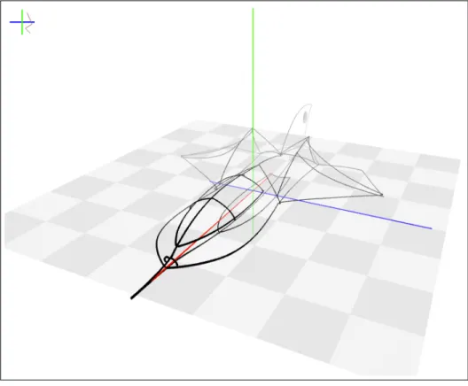
Figure 1.1: A jet fighter created using our system.
this trend are often called Sketch-Based Interfaces for Modeling (SBIM ). The motivation for an SBIM system is the ease of expressing one’s ideas with sketching and the significant flexibility of sketching over traditional WIMP paradigm. How computers will interpret the given sketch and produce a plausible 3D model, is the research question.
In this thesis, we present an SBIM method that tries to mimic the natural interface of pen and paper for creating 3D sketches (Fig. 1.1) that can be used as a starting point for a detailed 3D solid model, or simply an easier way to represent ideas in 3D without much effort. The system is designed to be as minimalistic and simple as possible, since it targets a broad range of users, from expert designers to naive users. There are two main concerns of the system. First is to minimize the learning time needed, yet still be flexible enough to create diverse free form 3D sketches. And second, to emphasize depth perception of the created objects by implementing several monocular depth cues, including motion parallax by tracking user’s head position. We test whether we are able to achieve these goals,
through several user tests (in Chapter 4: Evaluation, Results & Discussion). Our system is based on the very idea of curves, rather than 3D solid objects. Concern of creating surfaces not in mind, it is much easier to develop complicated 3D scenes and objects. Similarly, since the scene consists of only curves, users can easily predict what will be the outcome of drawing a certain stroke. Although there are several other examples of a similar 3D sketching interface, our contribu-tions to the field is to explain an easy to use 3D sketching tool, that is designed with less is more[41] thought in mind. A hybrid face tracking algorithm is also developed during the implementation of the system.
The rest of this thesis is organized as follows. Chapter 2 discusses the related work and the underlying motivation for our design decisions. The next chapter gives the details of our system in depth. Chapter 4 explains the user tests we conducted and gives a discussion of the results. Finally, Chapter 5 concludes the thesis by discussing how well we achieved our goals, and what can be done to improve the system further.
Our system has two distinct pipelines to work. These are Sketching (Section 3.2) and Face Tracking (Section 3.3.2). In order to better understand these com-ponents, one should learn the fundamentals of Sketch Based Modeling, Depth Perception, and Face Tracking. The upcoming subsections cover those areas in that order. Related Work of the system is detailed in Section 2.1.3.1.
2.1
Sketch Based Interfaces for Modeling
Sketch Based Interfaces for Modeling (SBIM) aims to create an automated (or
at least assisted) sketch-to-3D translation[42]. This trend is motivated by the expressiveness and ease of sketching.
The main concern of SBIM is to interpret the given sketch. There are two groups of interpretation an SBIM can make: using the sketch to create a 3D scene; or deforming/manipulating or adding details to an existing 3D model. Regardless of the goal, SBIM applications have a common pipeline (summarized in Fig. 2.1). The first step is sketch acquisition (Section 2.1.1) from user. Then, a filtering process (Section 2.1.2) is performed to clean the input, followed by interpretation of that input (Section 2.1.3) to a 3D operation.
Figure 2.1: The SBIM pipeline: First the input sketch is acquired and filtered. Then, the resulting smoothed input is interpreted as a 3D operation.
2.1.1
Sketch Acquisition
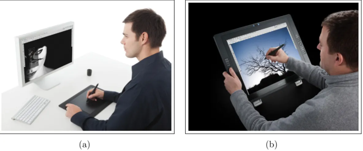
Getting the input sketch from the user is the most basic operation that needs to be performed by all SBIM applications. An input device for an SBIM system should allow freehand input. Even a standard mouse fits that broad description, but in reality devices that try to mimic the real pen and paper feel are much more suitable; such as pen tablets and recently tablet displays (Fig. 2.2(a)).
(a) (b)
Figure 2.2: SBIM systems acquire input from pen-based devices such as a pen tablet (a) or tablet display (b). (Wacom Bamboo and Cintiq, respectively.)
The benefit of a tablet display over a pen tablet is that the display is coupled with the input as well, providing even a better natural interaction.
coordinates. That positional information forms a piecewise linear approximation of the actual continuous gesture. The sample rate varies according to several factors, including but not limited to; drawing speed at a given time, or the input device’s model. Therefore, the sample points are not evenly spaced. The points tend to be closer when user moves his hand slower (e.g. corners), and further away when the gesture is faster (e.g. straight lines). This fact can be exploited to detect important parts of a drawing [48, 51].
(a) (b) (c)
Figure 2.3: (a) A stroke is performed by the user, (b) captures as a sequence of discrete points by pen device; (c) an image-based representation can also be used to represent the input. Reprinted from [42].
A time ordered sequence of input points that begins with a pen-down action and ends with pen-up is called a stroke (Fig. 2.3(a)). A sketch is the composition of many strokes. At bare minimum, a stroke is represented by a set of points, where every point p contains 2D coordinates (Fig. 2.3(b)). This information can be further enhanced by storing additional information such as the pressure that is applied to the pen at that point of time.
It is also possible to represent strokes with an image-based approach (Fig. 2.3(c)). Image-based stroke representation is mostly preferred by SBIM applications that aim to use the advantage of a fixed memory size and automatic
blending of strokes. One disadvantage of this approach is that, the temporal (i.e. time related) nature of the strokes is lost.
To be able to draw strokes to a 3D scene, the notion of a “drawing canvas” is introduced by several SBIM systems [21, 22]. Any Cartesian (e.g. x-y plane) or user-specified plane can become a drawing canvas, where the sketch is projected on. It is also possible to use non-planar surfaces as drawing canvas as well.
2.1.2
Sketch Filtering
A sketch needs to be filtered and smoothed before it can be interpreted, since the input is prone to be noisy and erroneous. There are two main sources for such noise: user and device error [52]. It is possible to end up with curves not that smooth, if the user is not proficient with drawing. Similarly, digitization of the input curve by the mechanical hardware may also induce noise. Therefore, it is essential to filter out noise by means presented below.
2.1.2.1 Resampling and Smoothing
As user’s drawing speed changes the distance between sampled points by input device also varies. Resampling that input data to even out distances is a way to reduce the noise (Fig. 2.4(a)). It can be done in real time by inserting new data points between further away sample points (i.e. interpolating), or by eliminating sample points that are too close to each other. Another approach for resampling is to apply a linear or smooth interpolation after the stroke gesture is finished.
Even a resampled input data does not guarantee a smooth curve. Therefore, it is necessary to further process input strokes to reduce discontinuities. A Gaussian filter[53] or a local averaging filter[1] can be applied to each sample point to achieve the desired effect.
(a) (b) (c)
Figure 2.4: Filtering operations: (a) smooth uniform resampling; (b) coarse poly-line approximation; (c) fit to a sppoly-line curve. Reprinted from [42].
2.1.2.2 Fitting
The number of sample points is still large after resampling and smoothing. It is important to simplify the input by fitting it to another representation. Polyline approximation is the easiest fitting that can be done, but the resulting output is not that representative (Fig. 2.4(b)). Curve fitting is the other option, which is the process of approximating the input point by means of curves, rather than lines (Fig. 2.4(c)). Obviously, curves are more representative.
There are a few different approaches of curve fitting. In general, parametric curve fitting such as Bezier[43], or B-spline[47] are more preferable than least-squares polynomial fitting[42]. One way to achieve a B-spline curve fitting is applying reverse Chaikin subdivision to generate the control points for the b-spline curve[17].
2.1.2.3 Over-sketching
When a user makes a mistake on the sketch, oversketching can be performed on the undesired region by carefully re-sketching it. The system is responsible for finding the affected region by over-sketching gesture and replacing it with the new input. The transition between old segments and the new segment should also be smoothed out (Fig. 2.6). It is possible to perform over-sketching in 2D, before the 3D interpretation [?].
(a) (b) (c)
Figure 2.5: Over-sketching: (a) initial curve; (b) oversketch gesture in red; (c) resulting curve.
several small overlapping strokes, rather than full-length smooth curves. Some SBIM systems can operate on such input by automatically blending these small strokes together to form a curve [?].
2.1.3
Sketch Interpretation
After sketch acquisition and filtering, the main step of an SBIM system is to interpret the sketch by mapping it to 3D. A freehand sketch input is open to several different interpretations, unlike selecting a menu item from drop-down menu. There are numerous open questions an SBIM system should answer. What is the user’s intention? Is the input valid? What is the correct way to map the input to a 3D operation?
There are many different interpretation of these questions, as expected. Olsen et al.[42] propose a taxonomy of SBIM systems to better explain these different interpretations. SBIM systems fall into two main categories. Those that try to fully create a 3D scene out of sketch input are called Model Creation Systems. And those that try to augment or deform an already existing 3D object with the guidance of the given input sketch can be grouped under Augmentation and
Deformation.
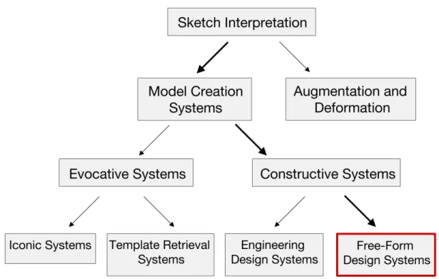
As explained, a model creation system aims to construct a 3D model or a scene from the 2D sketch input given by user. There are two distinct groups of model creation systems; Evocative Systems and Constructive Systems (Fig. 2.6). A constructive system tries to directly create the model out of the input strokes, whereas an evocative system merely uses these input strokes to come up with a
Figure 2.6: A taxonomy of sketch interpretation techniques. Our system fall in
Free-Form Design Systems under Constructive Systems for Model Creation
modified version of one of the built-in 3D model types that resembles the input. Constructive systems are harder to achieve than evocative systems, since the ambiguity of the input sketch can easily be reduced by the recognition step of an evocative system. On the other hand, the constructive systems need to recon-struct the 3D scene by just depending on the rules generated from input strokes alone. Since reconstruction is such a difficult problem, there are many diverse at-tempts to solve it. We can group these atat-tempts in two main groups; Engineering
Design Systems and Free-Form Design Systems.
Engineering design systems deal with hard-edged mechanical objects and sym-metrical properties. On the other hand, a free-form design system is mostly about (but not limited to) smooth, natural objects that need to be represented by curves, rather than straight lines. Since our system can be categorized as a Free-Form
Design System, we are going to explain the related work in this specific area in
2.1.3.1 Free-Form Design Systems
Creating free-form 3D objects and sketches from 2D user interfaces has been studied for a long time[9, 18, 59, 31]. Baudel et al.[9] describe a sketching interface for creating, manipulating and erasing curves in 2D, one of the oldest efforts. Cohen et al.[18] later propose an idea of creating 3D curves by drawing a 2D silhouette of the curve, and its shadow onto the surface. Unfortunately these invaluable efforts do not try to create a fully developed 3D sketch interface. Igarashi et al.[31] suggest such a true 3D scene creation tool later on.
(a) Bourguignon et al. (b) Kara et al.
(c) Tsang et al.
Figure 2.7: Related Work: (a) Bourguignon et al. (b) Kara et al. (c) Tsang et al.
There are recent studies on the subject that aim to enrich an already ex-isting 3D scene, either by annotating the scene or augmenting the 3D object itself[11, 34, 35, 55]. Bourguignon et al.[11] create such a system that can be used for both annotating a 3D object and creating an artistic illustration that
angle they make with the viewport. At Kara et al.[34, 35]’s work, a true 3D object is created by augmenting a simpler pre-loaded 3D template of the target object (Fig. 2.7(b)). The user then can edit this template 3D with a sketch inter-face. Similarly, Tsang et al.[55] use an image-based template to guide the users (Fig. 2.7(c)).
(a) Igarashi et al.s Teddy (b) Schmidt et al.s ShapeShop
(c) Nealen et al.s FiberMesh (d) Das et al.
Figure 2.8: Related Work (cont’d): (a) Igarashi et al.’s Teddy (b) Schmidt et al.’s ShapeShop (c) Nealen et al.’s FiberMesh (d) Das et al.
Several other studies focus on creating 3D solid objects using 2D sketches[31, 49, 40, 21]. Igarashi et al.’s Teddy[31] is one of the most well known 3D solid object creation systems. In this tool, users are able to create simple 3D objects by drawing 2D silhouettes of the target (Fig. 2.8(a)). Later this silhouette is inflated like a balloon to create the final 3D object. Schmidt et al.’s ShapeShop[49] can
be described as an extention to Teddy. ShapeShop supports three types of 3D object creation - “blobby” inflation in style of Teddy, linear sweeps and surfaces of revolution (Fig. 2.8(b)). Nealen et al.’s FiberMesh[40] is yet another extension to Teddy’s inflation system. However, unlike other systems, the user’s original stroke stays on the model to be used as a control curve for further editing (Fig. 2.8(c)). Finally, Das et al.[21] propose another system, where user strokes are interpreted as 3D space curves rather than 2D silhouettes. Using these curves, a 3D solid object is constructed (Fig. 2.8(d)).
Figure 2.9: Related Work (cont’d): Bae et al.’s ILoveSketch.
The approach we follow for 3D sketching is to ignore solid objects, and simply create scenes that only consist of 3D curves. The main advantage of such a system over 3D solid object creation is that it is easier to sketch complicated objects with full detail, since there is no concern about creating surfaces. Furthermore, it is easier for users to predict what will be the outcome of any stroke. Bae et al.’s
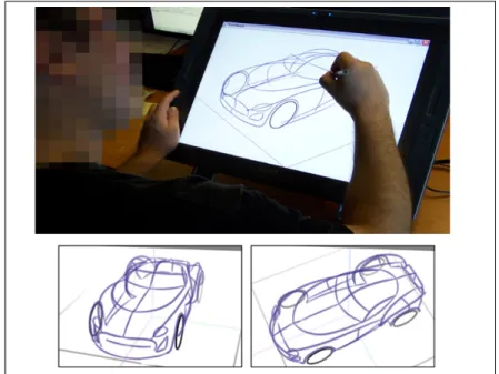
ILoveSketch[5], and later extended version EverybodyLovesSketch[6], rely on a
similar idea and allow users to create 3D sketches consisting of curves with the help of a pen display (Fig. 2.9). Bae et al.’s approach uses several different drawing tools that a user can select from: ortho plane (span), ortho plane (tick),
rotated V plane, oblique plane, extruded surface, freeform surface, 1-view epipolar surface, 2-view epipolar surface. Similarly, the system has several navigation
in depth[6]. Conversely, in our system we have chosen to use only a single way of drawing and navigating (as explained in Section 3.2.3), which makes it easier to learn.
2.2
Depth Perception
It is important to provide an accurate and informative depth perception during the design of a 3D scene. Depth cues establish the core of depth perception by helping human visual system to perceive the spatial relationships of objects. There are three main categories of depth cues[29]:
1. Oculomotor: Cues based on the position of our eyes and the shape of our lens.
2. Monocular: Cues that work with one eye. 3. Binocular: Cues that depend on two eyes.
2.2.1
Oculomotor Cues
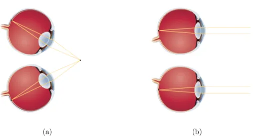
The oculomotor cues consist of Convergence, the notion of eyes being converged as we try to look at a nearby object, and Accommodation, the change in the tension of eye muscles (hence lens shape) that occurs when the distance of focus changes. The idea is that by feeling these changes at the eyes (the inward convergence and tight muscles), the human visual system can estimate the object distance (Fig. 2.10).
(a) (b)
Figure 2.10: Oculomotor Cues: (a) Convergence of the eyes and lens accommo-dation occurs when a person looks at something that is very close; (b) The eyes look straight ahead and the lens relax when the person observes something that is far away.
2.2.2
Monocular Cues
Monocular cues depend only on a single eye. They can be grouped into Pictorial
Cues, that can be extracted from a still 2D picture, and Movement Based Cues,
those related with the movement.
2.2.2.1 Pictorial Cues
Pictorial cues are those that can be perceived even from a static picture (Fig. 2.13). There are a number of different pictorial cues that we list below.
(a) Occlusion: Occlusion occurs when a farther away object is fully or partially blocked by another object that is closer to viewpoint (Fig. 2.13(a)).
(b) Relative Height: Object that are below the horizon and closer to the viewpoint have their bases lower than those farther away from the viewpoint (Fig. 2.13(b)).
Figure 2.11: Pictorial Cues: (a) occlusion (the road sign occludes the trees behind it); (b) relative height (the tree is higher in the field of view than road sign); (c) relative size (the far trees are smaller than the near one); (d) perspective convergence (the sides of the road converge in the distance); (e) atmospheric perspective (the far trees seem greyed out and less sharp). (Photography courtesy of Robert Mekis)
(g) (h)
Figure 2.12: Pictorial Cues (cont’d): (g) The location of the spheres are ambigu-ous; (h) Adding shadows makes their location clear. Notice the texture gradient on the ground as well. (Courtesy of Pascal Mamassion)
objects, the one farther away from the viewpoint will be perceived smaller and take up less of the viewport (Fig. 2.13(c)).
(d) Perspective Convergence: Perspective convergence dictates that the parallel lines extend out from the viewpoint will be perceived as converging at distance (Fig. 2.13(d)).
(e) Atmospheric Perspective: Atmospheric perspective causes distant ob-jets to be seen more blurry and less saturated with color (Fig. 2.13(e)). (f) Familiar Size: According to this cue, we can judge the distance of objects
based on our prior knowledge of their size.
(g) Shadows: Objects cast shadows which can provide information about the location of the object (Fig. 2.12).
(h) Texture Gradient: As distance increases, the elements get more closely packed with each other, even if they are actually at equal distances with their closer-to-viewpoint relatives (Fig. 2.12).
2.2.2.2 Motion-Produced Cues
Pictorial cues work even if the observer is in a stationary position. Once the observer or the objects start moving around, new cues emerge that further em-phasize depth.
(a) Motion Parallax: Motion parallax is the phenomenon that as we move, nearby objects move farther across our view volume than distant objects, which moves slower.
(b) Kinetic Depth Perception: Even if the observer is stationary, a motion based depth cue is still possible. Kinetic depth perception states that overall shape of an object can be better understand if the object rotates around its axis, eliminating ambiguities of 2D projection.
Figure 2.13: Motion Parallax: Notice how the image of the tree moves farther on the retina than the image of the house while eye is moving downwards.
2.2.3
Binocular Cues
(a) (b)
Figure 2.14: Binocular Disparity: (a) Notice the positions of the shapes being observed; (b) Binocular disparity happens between two eye images. Reprinted from [45].
In addition to monocular and oculomotor cues that depend on a single eye, there are also binocular cues, which are created by the differences in the images that is received by left and right eye. Binocular Disparity refers to that difference in the location of the object at left and right eye spheres. As object gets closer, disparity increases; and brain uses this information to extract depth information (Stereopsis).
2.3
Face Detection and Tracking
As we mention in previous section, motion based cues are fundamental for better perceiving depth information. Such a kinetic depth effect can be achieved by means of tracking the user’s face with the help of a camera. The first step that needs to be done for the tracking is Face detection. Face detection is one of the fundamental approaches for a natural human computer interaction. It is the basis algorithm for several facial analysis techniques, including but not limited to facial expression recognition, face verification, face modeling and in our case face tracking.
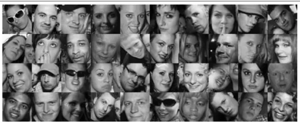
For a given arbitrary image, the face detection algorithm aims to answer the existence of any faces in the image, and their positions if they do exist[57]. Although the definition of the problem sounds primitive, the solution is not. Therefore, face detection is one of the top studied topics for computer vision. The significance of the problem lies in the several variable attributes a face has; including scale, location, pose, expression, lighting and etc. (Fig. 2.15).
Figure 2.15: Different face poses. Note the variation in pose, facial expression, lighting and etc. Reprinted from [44].
There are several different approaches to face detection. The early approaches (before 2000s) are surveyed in [57] and [30] in detail. Since the face detection is merely a tool for the greater purpose of achieving a depth perception aware sketching tool, there is no need to explain those solutions in depth. Yang et al.[57]
Feature invariant approaches aim to match structural face characteristics that are not affected by environmental variables such as pose or lighting. Knowledge-based methods assume predefined rules that are Knowledge-based on several common-sense rules about a human face to detect it. In a template matching approach, there is a face template which is compared against the target image. And finally, appearance based methods use a large dataset of various face images to train a face detector. In general, appearance based methods perform better than all the rest.
The detection algorithm that we use in our system is also an appearance based method. Developed by Viola and Jones[56], the algorithm actually made it practically possible to detect faces in real time. As stated at [60], Viola and Jones’ algorithm is the “de-facto standard of face detection”.
2.3.1
Viola-Jones Face Detector
The success of Viola-Jones Face Detector depends on three fundamental ideas: the
integral image, AdaBoost learning algorithm, and the attentional cascade struc-ture.
2.3.1.1 The Integral Image
Integral image (a.k.a. summed area table) is an algorithm to compute the sum of values in a sub-rectangle of a grid rapidly and efficiently. Crow et al.[20] first proposed the idea of integral image for use in mipmaps. Later, Viola and Jones applied the same principle to quick computation of Haar-like features. The details of the process are below.
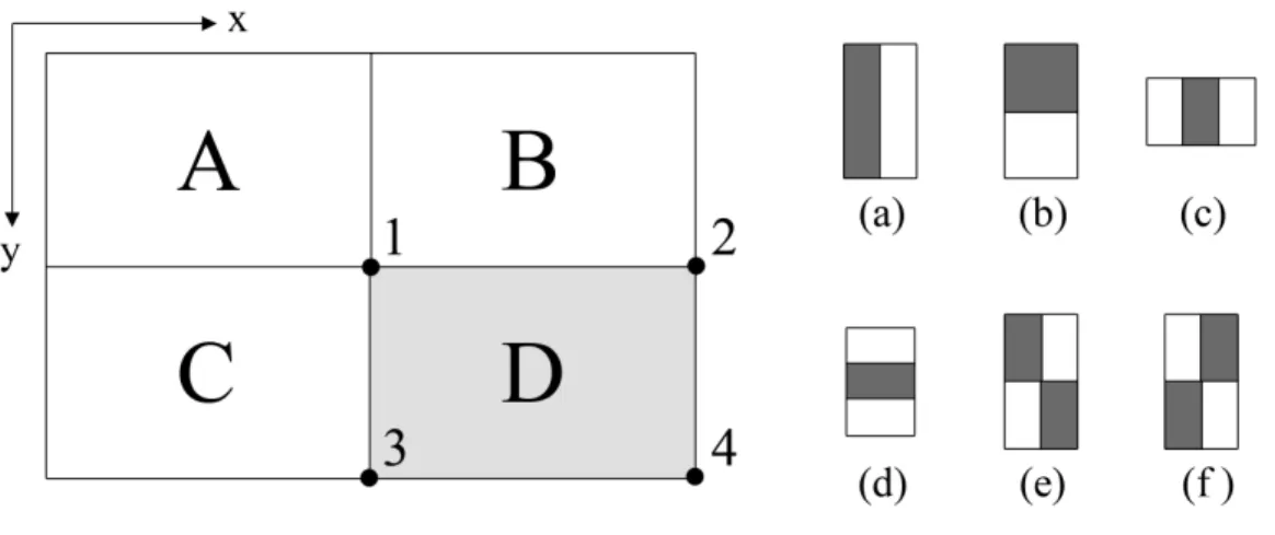
Figure 2.16: Integral image computation and Haar-like rectangle features (a-f). The sum of the pixels within rectangle D computed with four array references. The value of the integral image at location 1 is the sum of the pixels in rectangle
A. The value at location 2 is A + B; at location 3, it is A + C; and at location
4, it is A + B + C + D. Therefore, the sum for rectangle D can be computed as 4 + 1− (2 + 3).
ii(x, y) = ∑
x′≤x,y′≤y
i(x′, y′) (2.1) where ii(x, y) is the integral image value, and i(x′, y′) is the original image value for pixel location (x, y). Using the below two recursions,
s(x, y) = s(x, y− 1) + i(x, y) (2.2)
ii(x, y) = ii(x− 1, y) + s(x, y) (2.3) the integral image can be computed in a single pass using dynamic programming.
s(x, y) in the equations is the cumulative row sum, where s(x,−1) = 0, and ii(−1, y) = 0.
The sum of any sub-rectangular area can easily be computed using the integral image (Fig. 2.16). For instance, the sum of pixels in rectangle D is,
∑ (x,y)∈D
tures, as shown in Fig. 2.16(a-f). A feature is simply the intensity difference between two separate rectangular regions. For instance, the feature value (a) is computed as the difference between the average pixel value of gray and white rectangles. Since there are two common corners for these two rectangles, only six references are needed to perform the computation. Similarly, features c and
d require eight, features e and f require nine array references.
2.3.1.2 AdaBoost Learning Algorithm
There are many ways of learning a classification function, given a training set of positive and negative images and a feature set to derive. Boosting is one of such classification methods. It is the procedure of combining several weak classifiers to achieve an accurate hypothesis, hence called boosting. For a general introduction on boosting, one can read references [27] and [39]. One of the typical boosting algorithms that is also recognized as the first step of several others is the Adaptive Boosting (AdaBoost ) algorithm[26]. Viola-Jones uses AdaBoost to select a small set of features and train the classifier.
There are hundreds of thousands of Haar-like rectangular features for each image sub-rectangle, significantly more than the total number of pixels. Although the computation time for a single feature is not that exhaustive, computing the complete set of features is practically not possible. Therefore, the Viola-Jones algorithm aims to compute a fine tuned sub-set of features, which creates an effective classifier once combined. The main challenge is, of course, to find these features.
To achieve this, the single Haar-like feature that best separates positive sam-ples from negatives is selected at the weak learning algorithm. For every feature, the weak learning algorithm adjusts the optimal threshold, such that the min-imum number of examples are misclassified. In essence, a weak learner hj(x)
1. Given example images (x1, y1), . . . , (xn, yn) where yi = 0, 1 for negative and positive examples respectively.
2. Initialize weights w1,i = 2m1 ,2l1 for yi = 0, 1 respectively, where m and l are the number of negatives and positives respectively.
3. For t = 1, . . . , T :
(a) Normalize the weights,
wt,i ←
wt,i ∑n
j=1wt,j
(2.5)
(b) For each feature j, train a classifier hj which is restricted to using a single feature. The error is evaluated with respect to wt, ϵj = ∑
i|hj(xi)− yi|.
(c) Choose the classifier ht, with lowest error ϵt. (d) Update the weights:
wt+1,i = wt,iβt1−ei (2.6) where ei = 0 if example xi is classified correctly, ei = 1 otherwise, and βt= 1−ϵtϵt .
4. The final strong classifier is:
h(x) = { 1 if ∑Tt=1αtht(x)≥ 12 ∑T t=1αt 0 otherwise (2.7) where αt= log β1t
Algorithm 1: The AdaBoost algorithm selects a single feature from the hundreds
where fj is a feature, θj is the optimal threshold for that feature, and pj is the parity to adjust the direction of inequality. See Algorithm 1 for a summary of the complete boosting process.
2.3.1.3 The Attentional Cascade
Attentional cascade plays an important role in the Viola-Jones detector. As stated in [56], “the key insight is that smaller, and therefore more efficient, boosted
classifiers can be constructed which reject many of the negative sub-windows while detecting almost all positive instances”. In other words, it is possible to adjust
the threshold for each boosted classifier so that false negative rate is almost zero. That will lead to the rejection of most sub-windows with false positives in an early stage of the pipeline, making it extremely efficient.
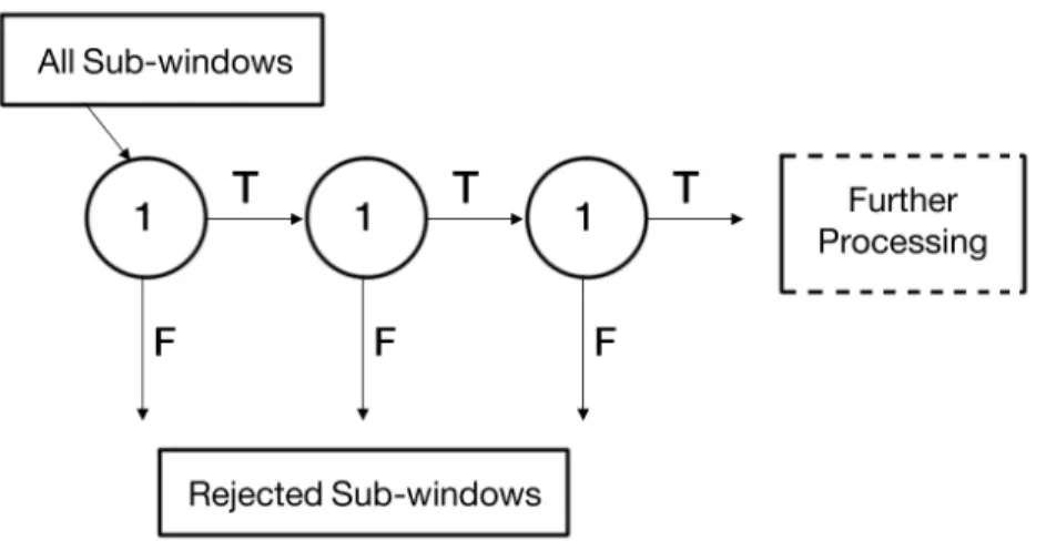
Figure 2.17: Schema of the detection cascade. A pipeline of classifiers are applied to every sub-windows of the image. The classifier get more complex as we pro-ceed at pipeline (i.e. number of weak classifiers that are involved for each node increases for latter nodes). The initial classifier trained to eliminate a massive number of negative examples with very low number of weak classifiers. After sev-eral stages of processing the number of candidate sub-windows have been reduced radically.
The process for classification of a sub-window forms a special case of a deci-sion tree, which is referred as a “cascade” in [56]. The input sub-window proceeds through a pipeline of classifier nodes for detection, as shown in Fig. 2.17. Each classifier will make a binary decision on whether a sub-window is a false negative (i.e. reject), or not (i.e. proceed to next node). The number of weak classifiers involved for each node increases as image continues its journey at the pipeline (e.g. the first five nodes include 1, 10, 25, 25, and 50 weak classifiers, respec-tively [56]). This is an expected schema, since it gets more and more difficult to reject all negative windows while keeping positive samples at later stages. The notion of having fewer number of weak classifiers at first nodes also improves the performance of the Viola-Jones detector.
The training process is also affected by the cascade structure as well. Since a positive sub-window is a rare incidence, usually billions of negative samples are needed to build a successful face detector. Viola and Jones uses a bootstrap process to handle this need. The false positive rate should be reduced at each stage of the attentional cascade. A threshold is manually chosen for the minimum reduction in the false positive rate. Then, each stage of the cascade is trained by adding weak classifiers until the threshold of false positive rate is met. More and more stages are added to the final cascade until the overall target for detection rate and false positive rate is achieved.
Viola and Jones[56] trained the attentional cascade manually as described above (i.e. the decision thresholds and the number of weak classifiers are selected manually). Given the limited computational power available at that time, it is no surprise that constructing a well performing face detector requires a significant tuning effort..
2.3.2
Continuously Adaptive Mean Shift
The Continuously Adaptive Mean SHIFT (CamShift) algorithm[14], is a
deriva-tion of the Mean Shift algorithm[19], a robust non-parametric iterative technique for finding the mode of probability distributions[25].
CamShift algorithm is summarized at Fig. 2.18. At every video frame, a color probability distribution image is created for the actual frame image via a color histogram model of the color being tracked (i.e. skin color for face tracking). CamShift algorithm operates on the probability image to locate the center and the size of the object being tracked. The last size and location is used as the search window for the next video image. That process is repeated for every frame, hence a continuous tracking is performed. As previously noted, the CamShift algorithm is an extension to the Mean Shift algorithm (Fig. 2.18).
2.3.2.1 How the Mean Shift Algorithm Works
The Mean Shift algorithm is the core part of the CamShift algorithm. It is per-formed on a color probability distribution image that is produced from histogram back-projection:
1. Decide the size of the search window.
2. Decide the initial location for the search window.
3. Compute the location of the mean value in the search window.
4. Adjust the search window’s center as the mean location computed in pre-vious step.
5. Repeat Steps 3 and 4 until convergence. (i.e. until the search window’s center has moved less than a predefined threshold.)
For a discrete image probability distribution, the location of the mean value in a search window (Steps 3 and 4 above) can be found as follows:
a. Find the zeroth moment,
M00 = ∑ x ∑ y I(x, y) (2.9)
c. Find the mean search window location as, xc = M10 M00 ; yc= M01 M00 (2.11) where I(x, y) is probability at the position (x, y) in the image, and x and y range over the search window.
2.3.2.2 How the Continuously Adaptive Mean Shift Algorithm Works
CamShift is designed for dynamic distributions, unlike the Mean Shift algorithm, which is for static distributions. Change in the distribution occurs when the tracked object moves in a video sequence so that the size and location of the probability distribution changes as well. The goal of the CamShift algorithm is to adjust the search window (both size and location). The initial window size can be set to any reasonable value. In our case, we set the initial location and size of the window using Viola-Jones Face Detector[56]. Using this initial window, CamShift continuously adapts its new window size and location for each video frame, as follows[37]:
1. Set the calculation region of the probability distribution to the whole image. 2. Choose the initial location of the 2D mean shift search window.
3. Calculate the color probability distribution in the 2D region centered at the search window location in an ROI slightly larger than the mean shift window size.
4. Run mean shift algorithm to find the search window center. Store the zeroth moment (area or size) and center location.
5. For the next video frame, center the search window at the mean location stored in Step 4 and set the window size to a function of the zeroth moment found there. Go to Step 3.
For each frame, the Mean Shift algorithm will tend to converge to the mode of the distribution. Therefore, CamShift for video will tend to track the center (mode) of color objects moving in a video scene.
Users interact with our system using a pressure sensitive pen tablet. In essence, users’ pen gestures are captured as time sequenced tablet coordinates and in-terpreted. The device has several buttons on the tablet that are used for basic non-gestural abilities such as undo, redo, toggle symmetry. The pen also has two buttons, and an eraser at back, that are used as toggles between our ges-ture modes as detailed in the Section 3.2.3. To be able to give users a real pen and paper experience, our system does not use any of the elements of WIMP (windows, icon, pointer, and menu) paradigm, hence creating a natural interface where users complete tasks simply interacting with the system as if it’s a real paper.
Depth perception is another aspect that we consider when building the system. As detailed in Section 3.3, we implement several pictorial cues to emphasize the perception of depth throughout the system. We also track the user’s head position to manipulate the position and direction of the virtual camera at the scene, creating a motion parallax based kinetic depth effect.
3.1
Overview
Our system consists of three modules: sketching, face tracking, and rendering, as pictured in Fig. 3.1. Every module is responsible for a different aspect of the system.
Figure 3.1: Overview of the system. Three modules work together to get sketch input from user, and visualize that sketch emphasizing depth perception with the help of face tracking enabled motion parallax.
The sketching module collects input strokes from user with the help of a pen tablet. The collected input strokes are then filtered and interpreted as explained
a camera. By applying a hybrid tracking, the face tracking module enables the
virtual camera to travel orbitally along the scene. Finally, the rendering step
uses pictorial depth effects to accurately visualize the current scene for the given viewpoint. Since face tracking and rendering modules are solely responsible for the “visualization” of the system, we are going to discuss the details of these systems in Section 3.3.
(a) (b) (c)
(d) (e) (f)
Figure 3.2: Overview of the usage. (a) User adjusts the plane that he wants to draw a curve on. (b) User draws the curve using pen tablet, which is mapped to the current drawing plane. (c) The input curve is then re-sampled and smoothed out. (d) User can change the camera position if he needs to. (e) This process is repeated until the desired 3D sketch is formed. (f ) Final result; a cube.
Fig. 3.2 illustrates the overall usage of the system. To be able to draw a curve, the user firsts adjust the drawing plane as explained in Section 3.2.3. Any drawing gesture that is made by the user will be reflected on this surface. Once the drawing plane is adjusted, the user can draw a curve with a simple pen gesture on the tablet. The input curve will then be re-sampled and smoothed using the
algorithms described at Section 3.2.2. During this process, the user can adjust camera position as well, using the same pen tablet device, if necessary. The user can repeat these steps to complete the 3D object.
3.2
Sketching Pipeline
There is a common pipeline as explained in Section 2.1 for sketch based interfaces, which our system also follows. The first step is to acquire input from the user (Section 3.2.1), by means of an input device, a pen tablet in our case. That step is followed by sketch filtering (Section 3.2.2), where the data is re-sampled and smoothed. Finally, the sketch is interpreted appropriately. In our case, interpretation means mapping these curves one of many gestures explained in Section 3.2.3.
3.2.1
Sketch Acquisition
Obtaining a sketch from the user is the first step a sketch based interface should perform. Our system collects free hand sketches from the user using a pen tablet. A tablet display would be even a better choice, since the user will be able to see what he draws just at the drawing surface he is using.
There are basically two different ways of storing a sketch from the user. Either it can be stored as time-ordered sequence of points (i.e. a stroke), or approxi-mated to an image based representation[42]. Since we want to preserve temporal information, stroke based approach is better suited than image representation for this purpose.
3.2.2
Sketch Filtering
It is important to perform filtering before storing a sketch to the system, since there will be some error caused by both user and the input device itself[50]. The
always exist. Therefore, the input data should be interpreted knowing that it is imperfect. To overcome this imperfection, our system applies below approaches:
(a) (b) (c)
(d) (e) (f)
Figure 3.3: Re-sampling and Smoothing. (a) A user input would look like this before any re-sampling and smoothing (b) The distance between data points is not equal to each other. (Total of 706 points) (c) To make those distances even, the input data is re-sampled (Total of 2877 points) (d) A Gaussian filter is applied on the fly as well. (e) Reverse Chaikin subdivision is applied to simplify curve representation and further smoothing (Total of 47 points used to represent the curve) (f ) Final result; a smooth B-spline curve (Total of 188 points is used to render the curve).
3.2.2.1 Re-sampling and Smoothing
The distance between consecutive data samples that are acquired from the pen tablet is not always the same (Fig. 3.3(b)). Because of this, data points that are sampled closer than a given threshold should be discarded. Similarly, if there is any data point that is sampled too far from the previous point, a interpolation
must be performed between these two data points. In our system, this re-sampling is actuated on the fly (Fig. 3.3(c)). However, re-sampling is not sufficient alone. To further smooth out the given input, we use a local Gaussian filter (Fig. 3.3(d)) to any upcoming data point (i.e. the newly acquired data point is adjusted according to a Gaussian filter applied to that point and neighboring points)[54].
1. Calculate the adjusted position pf of a newly added point Pf as,
pf = w∑i>ϵ i=0 wipi (3.1) wi = f (i, µ, σ2) (3.2) f (i, µ, σ2) = 1 σ√2πe −1 2( x−µ σ ) 2 (3.3) where µ = 0 and σ2 = 1, hence weight function w
i is a standard normal
distribution; and pi is the ith neighboring point’s current location. 2. Notice sum iterates as long as wi is greater than a small number (i.e. It
iterates for 4-5 times).
Algorithm 2: The Gaussian filtering step. A standard normal distribution is
used as a weighting function for neighboring points to adjust newly added point’s final location.
The details of the Gaussian filtering step is explained at Algorithm 2. Basi-cally, we use a standard normal distribution to decide on the weights assigned to each neighboring point of the newly added point. We adjust this new point by the calculated weighted average.
3.2.2.2 Fitting
After re-sampling and smoothing is performed, the resulting curve consists of hundreds of data points. To simplify this representation, we fit a curve onto these data points, using Reverse Chaikin Subdivision[8]. Reverse Chaikin Subdivision is a standard algorithm to produce less number of coarse points that will represent
we concluded that six iterations are suitable for our case. Assuming fine points are denoted as p1,p2,...,pn, and coarse points are denoted as c1,c2,...,cm, a coarse point cj can be computed as:
cj =− 1 4pi−1+ 3 4pi+ 3 4pi+1− 1 4pi+2 (3.4)
where the step size of i variable is two (hence halving the cardinality of the fine points).
3.2.3
Sketch Interpretation
After input sketch is acquired and filtered, the last step of the sketching pipeline is to interpret the given stroke. In our system, the pen tablet acts like a gestural
interface for users, allowing it to be used for several different tasks. The user can
switch between different modes by holding down the buttons on the pen. During a regular session with the system, one will use the pen for camera adjustment, plane selection, drawing, erasing and editing. Hence the detected input stroke will be mapped to one of these gestures, as explained below.
3.2.3.1 Camera Adjustment
When the pen is in this mode, every movement that the user does will be mapped to an invisible Two-Axis Valuator Trackball [16]. The horizontal pen movement is mapped to a rotation about the up-vector, whereas a vertical pen movement is mapped to a rotation about the vector perpendicular to view and up, as explained at Algorithm 3. Any diagonal movement is also easily mapped to a combined rotation (Fig. 3.4). As Bade et al. suggest[4], Two-Axis Valuator Trackball is “the best 3D rotation technique” among several other rotational widgets.
1. Calculate normalized x and y offsets ∆xn and ∆yn as, ∆xn=
xcurrent− xinitial
screenW idth , ∆yn =
ycurrent− yinitial
screenHeight (3.5)
2. Given ⃗Si is the initial view point position at spherical coordinate system, current view point position ⃗Sc =⟨Sc,x, Sc,y, Sc,z⟩ becomes,
⃗
Sc= ⃗Si+⟨−∆xnπ, ∆ynπ, 0⟩ (3.6) 3. Using spherical coordinate ⃗Sc, the current position in Cartesian
coordi-nate system ⃗Cc=⟨Cc,x, Cc,y, Cc,z⟩ can easily be computed as,
Cc,x = Sc,z× sin(Sc,y)× cos(Sc,x) (3.7)
Cc,y = Sc,z × cos(Sc,y) (3.8)
Cc,z =−Sc,z× sin(Sc,y)× sin(Sc,x) (3.9) 4. When camera adjustment gesture is finished (i.e. pen is lifted up from
tablet), update initial spherical view point position as,
Si = Sc (3.10)
Algorithm 3: Two-Axis Valuator Trackball. The normalized offset of the
cur-sor is used to calculate current spherical coordinates, which is the step before calculating real Cartesian coordinates.
Figure 3.4: Camera adjustment. Any pen movement is mapped to an invisible Two-Axis Valuator Trackball.
a virtual surface in the 3D scene. To enable this effect, the user should select a drawing plane beforehand. In our system, there are only two distinct ways of selecting the drawing plane.
(a) (b) (c)
(d) (e)
Figure 3.5: Plane selection. (a) The plane that selected curve lies. (b) The plane that’s tangential to the selected curve and perpendicular to its plane. (c) The plane that is perpendicular to both (a) and (b). (d) The Cartesian coordinate system that is formed by those three planes. (e) The plane that is adjusted by extruding a picking ray from the current viewpoint. This plane is parallel to current viewport’s near plane.
• In the first available approach, the user takes an assistance from coordinate
system lines and current curves on the scene. By selecting any of these curves and lines, the user changes the drawing surface as the plane that
selected curve lies in (Fig. 3.5(a)). Further flexibility is enabled with the help of toggle plane button on the tablet. Once that button is pushed, the drawing surface will be changed to the plane that’s tangential to the selected curve from the selection point, and perpendicular to the plane that the curve lies (Fig. 3.5(b)). Another toggle will change the drawing surface once more, this time as the plane that is perpendicular to both the first plane and the tangential plane (Fig. 3.5(c)). By the help of such three planes, the user can form a mental model of the Cartesian coordinate system at any position and orientation (Fig. 3.5(d)).
• To support even more flexibility, we realized a second approach to plane
selection. In this method, the user can adjust the drawing surface to a plane that is parallel to the current near plane of the scene’s viewport, and
x distant from that near plane, where that x is determined by the current
pressure on the pen (Fig. 3.5(e)).
3.2.3.3 Drawing
(a) (b)
Figure 3.6: Drawing. (a) User can draw arbitrary shaped curves (b) Snap points can help to create connected curves.
The main functionality of the system is drawing curves (Fig. 3.6(a)). In this mode, the user can simply draw several curves using the pen tablet. The time
in Section 3.2.2. Finally, a B-Spline curve is fitted to the stroke data. While in the drawing mode, the user can take advantage of snap points that will appear at the start and end points of existing curves (Fig. 3.6(b)). These snap points make it easier to draw closed or connected shapes.
3.2.3.4 Erasing
(a) (b)
Figure 3.7: Erasing. (a) User selects the curve to be erased. (b) Performs the erasing with simply turning over the pen and erasing the part he wants.
A paper and pen system cannot be imagined without an eraser. The user can simply turn over his pen device to switch to the eraser mode. Once this is done, the cursor on the screen will get larger to mimic an eraser functionality. Since in a crowded scene, there will be several curves that will lie under eraser’s cursor, it will be harder to erase a specific curve’s segment. Therefore, erasing can only be performed on the current selected curve (Fig. 3.7).
(a) (b)
Figure 3.8: Editing. (a) User selects the curve to be edited, and draws the edit curve. (b) Final result.
3.2.3.5 Editing
Sometimes, the user may want to edit a section of a curve that has a minor flaw. In such a situation, it may be appropriate to use the editing tool instead of erasing that part and re-drawing. Just as in erasing tool, editing is also only performed at the current selected plane (Fig. 3.8).
Over-sketching is a commonly used gesture, when there is a curve region that needs to be corrected. Once a secondary stroke is drawn, the system can update the initial curve by slicing it into segments, and replacing the old segment with the new stroke. A smoothing algorithm is also performed between the transitions of these segments. We use Fleisch et al.[24]’s algorithm to over-sketching that is explained in Algorithm 4.
3.2.3.6 Miscellaneous Operations
As mentioned, there are also several buttons on the tablet, that can be used to achieve miscellaneous operations. When symmetry is toggled, using one of these buttons, any gesture that is performed with the pen will also be reflected to the symmetry of that gesture. For instance, if a curve is drawn when the
1. The algorithm replaces curve segment Cd with the newly sketched seg-ment Co, resulting in Cr where,
Cd = (x0, x1,· · · , xn),
Co = (y0, y1,· · · , ym),
Cr = (r0, r1,· · · , ro)
(3.11)
2. The start xs and end xe points of the segment are found by finding the minimum distance between xi and y0 and ym as,
xs = min(|xi− y0|), i = 0, · · · , n,
xe = min(|xi− ym|), i = 0, · · · , n
(3.12)
3. The resulting curve then contains the points,
Cr = (x0,· · · , xs−1, y0,· · · , ym, xe+1,· · · , xn) (3.13) 4. The resulting curve is further smoothed to reduce hard breaks. To do that, the smoothing equation below is applied to m2 neighbors from start and end points of over-sketched segment, where m is the length of that segment:
xt= xt+ (y0− xs)× (0.5 × sin(t + 0.5π) + 0.5) (3.14) where either s− 1 −m2 < t < s− 1, or e + 1 < t < e + 1 + m2
Algorithm 4: Constraint Stroke-Based Oversketching for 3D Curves. Reprinted
symmetry is enabled, a symmetric curve will also be created. Similarly, if a part of a curve will be erased while symmetry is enabled, the same part will be erased for its symmetric counter as well. Symmetry is important to product design, since people prefer objects with symmetry, unity and harmony[10].
To prevent errors that the users might make, the system changes the pen’s cursor’s image to reflect the current gesture mode[3]. For instance, it’s a single dot for drawing, a slightly bigger red circle for editing, a cross-hair for plane selection etc. Similarly, our system also supports undo/redo actions using the tablet buttons as well. This functionality is essential for basic error recovery. As can be seen in Section 4, undo is widely used among our users.
3.3
Visualization Pipeline
Correct visualization of a scene is fairly important to make it easier for users to understand the 3D information at the scene. As in real world, computer generated scenes take advantage of depth cues to emphasize 3D. Out of three groups of depth cues (oculomotor, monocular, binocular), monocular depth cues are possible to implement using a standard computer display. One should use stereo-displays or anaglyph rendering if the aim is to benefit binocular cues as well.
Since our system also uses a generic computer display, we used monocular depth cues for 3D visualization. We have a few simple algorithms about pictorial
cues explained further in the upcoming section (Section 3.3.1). We also tracked
user’s face to achieve kinetic depth effect using motion parallax, hence empha-sized motion-based cues. The details of face tracking approach is explained in Section 3.3.2.
with the help of so called pictorial cues. There are several studies that have aimed to explain the interaction of depth cues when several of them are present within a scene. Some of these studies propose that depth cues are combined in an additive fashion[33, 32, 58], others suggest there is a non-linear relation between different depth cues[12, 46]. Whether linear or non-linear, one aspect all these studies seem to agree is that multiple depth cues help disambiguation of the visual stimuli and with the more depth cues, the better the depth perception of the observer[28].
With this reasoning in mind, we have attempted to implement as many non-conflicting depth cues as possible. The resulting effect is almost identical to the one that we expect from a real world scene. As demonstrated at Fig. 3.9, rendered from a similar viewpoint; our system emphasizes the same pictorial cues as does the real world image: occlusion, relative height, relative size, perspective convergence, and atmospheric perspective.
Perspective projection is actually responsible for some of these pictorial depth cues, and we did not have to take any special measures for it. These pictorial cues are occlusion, relative height, perspective convergence, and texture
gradient. One can expect that relative size should be listed as a
perspective-projection-resulted depth cue. But that is not the case for our system. The scenes we create consist of mere line polygons, and OpenGL does not adjust the line width according to depth. Therefore propose a solution, as explained in Algorithm 5. At every render loop, we are calculating the distance of each line from the viewpoint. Then using the normalized distance value, we are setting a proper line width and color for that line segment. The change in width results in
relative size, while the change in color emphasizes atmospheric perspective
(Fig. 3.10).
This idea is also supported by technical illustrators. In technical illustration, there are three line conventions suggested by Judy Martin[38]: use single line weight throughout the image; use heavy line weights for out edges, and parts
(a) A real world scene demonstrating pictorial depth cues
(b) A 3D replica of the same scene at our system.
Figure 3.9: A 3D replica of a real world scene at our system. Notice how we preserved pictorial depth cues at rendering; (a) occlusion, (b) relative height, (c) relative size, (d) perspective convergence, (e) atmospheric perspective