Inertial/Magnetic Sensor Units
Kerem Altun and Billur BarshanDepartment of Electrical and Electronics Engineering Bilkent University, Ankara, Turkey
{kaltun,billur}@ee.bilkent.edu.tr
Abstract. This paper provides a comparative study on the different techniques of classifying human activities that are performed using body-worn miniature inertial and magnetic sensors. The classification tech-niques implemented and compared in this study are: Bayesian decision making (BDM), the least-squares method (LSM), thek-nearest neighbor algorithm (k-NN), dynamic time warping (DTW), support vector ma-chines (SVM), and artificial neural networks (ANN). Daily and sports activities are classified using five sensor units worn by eight subjects on the chest, the arms, and the legs. Each sensor unit comprises a tri-axial gyroscope, a tritri-axial accelerometer, and a tritri-axial magnetometer. Principal component analysis (PCA) and sequential forward feature se-lection (SFFS) methods are employed for feature reduction. For a small number of features, SFFS demonstrates better performance and should be preferable especially in real-time applications. The classifiers are val-idated using different cross-validation techniques. Among the different classifiers we have considered, BDM results in the highest correct classi-fication rate with relatively small computational cost.
Keywords: inertial sensors, magnetometers, human activity recogni-tion and classificarecogni-tion, feature selecrecogni-tion and reducrecogni-tion.
1
Introduction
Computers have been in peoples’ lives for many decades. With rapidly accel-erating technology, hand-held computers have already made their way to our daily lives. Human-computer interaction has been an active research area since the introduction of computers; however, it is now becoming essential to design context-aware systems that recognize and interpret human behavior correctly. One aspect of human behavior understanding is the recognition and monitoring of daily activities. A wearable activity recognition system can improve the qual-ity of life in many critical areas, such as ambulatory monitoring, home-based rehabilitation, and fall detection.
Earlier activity recognition systems mostly used vision as the sensing modal-ity [1,2] and that track of research is still going on today [3]. However, vision-based systems can only be used in a confined space, e.g., a house, an office, or A.A. Salah et al. (Eds.): HBU 2010, LNCS 6219, pp. 38–51, 2010.
c
a laboratory, with carefully adjusted environmental parameters such as proper illumination. Using cameras can also interfere with the privacy of the individual in question and this may even cause him/her to act differently than normal. Furthermore, when a single camera is used, the 3-D scene is projected onto a 2-D one, with significant information loss. Occlusion or shadowing of points of interest (by human body parts or objects in the surroundings) is circumvented by positioning multiple camera systems in the environment and using several 2-D projections to reconstruct the 3-D scene. This requires each camera to be separately calibrated.
It is said in [4] that “Activity can be best measured where it occurs.” Miniature inertial sensors can be flexibly used inside or behind objects without occlusion ef-fects. This is a major advantage over visual motion-capture systems, that require a free line of sight. Because of such restrictions, alternative activity recognition systems, mostly using wearable miniature inertial sensors are being developed. References [5,6,7] provide comprehensive surveys on the use of inertial sensors in motion recognition and analysis.
Inertial sensor based activity recognition systems are used in monitoring and observation of the elderly remotely by personal alarm systems [8], detection and classification of falls [9,10], medical diagnosis and treatment [11], monitor-ing children remotely at home or in school, rehabilitation and physical ther-apy [12], biomechanics research [7], ergonomics [13], sports science [14], ballet and dance [15], animation, film making, TV, live entertainment, virtual reality, and computer games [16].
Vision-based systems and inertial sensor based systems are by no means exclu-sive; in a number of studies, video cameras are used as a reference for comparison with inertial sensor data [17,18,19], whereas in some studies the vision data is integrated or fused with inertial sensor data [20]. Fusion of inertial sensors with magnetometers is also reported in the literature [18,21].
In inertial sensor based systems, there has not been a universal agreement on the number and types of sensors to use, positioning of the sensors, and the methods to use for recognition. Some studies distinguish between postures, i.e., sitting, standing, and lying using the static component of acceleration [8,17,22], whereas some distinguish between as many as 20 activities [22]. Some studies also recognize transitions between postures [8,19,23,24]. The number of sensors used vary between one [8,23] to twelve [4]. To the best of our knowledge, techniques that optimally determine the number, types, and positions of sensors do not exist [22].
This paper presents the results of a comparative study on human activity recognition, using accelerometers, gyroscopes, and magnetometers. We use five sensor modules, each of which includes a triaxial accelerometer, a triaxial gyro-scope, and a triaxial magnetometer. We compare the successful differentiation rates, reliability and repeatability of the results, and computational requirements of various classification techniques using two different feature reduction methods.
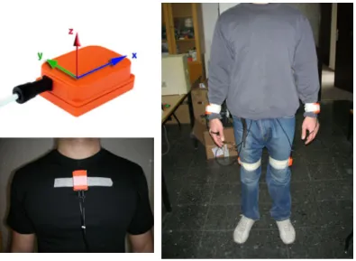
Fig. 1. Xsens sensor modules and their positioning on the body
2
Classified Activities and Experimental Methodology
The 19 activities that are classified using body-worn miniature sensor units are: sitting (A1), standing (A2), lying down on back and on right side (A3 and A4), ascending and descending stairs (A5 and A6), standing in an elevator still (A7) and moving around in an elevator (A8), walking in a parking lot (A9), walking on a treadmill with a speed of 4 km/hr (in flat and 15◦ inclined positions) (A10 and A11), running on a treadmill with a speed of 8 km/hr (A12), exercising on a stepper (A13), exercising on a cross trainer (A14), cycling on an exercise bike in horizontal and vertical positions (A15 and A16), rowing (A17), jumping (A18), and playing basketball (A19).Five MTx 3-DOF orientation trackers are used, manufactured by Xsens Tech-nologies [25]. Each MTx has a triaxial accelerometer, a triaxial gyroscope, and a triaxial magnetometer so that the sensor units acquire acceleration, rate of turn, and Earth-magnetic field data, all in 3-D.
Accelerometers of two of the MTx trackers can sense up to±5g and the other three can sense in the range of±18g, where g = 9.80665 m/s2is the gravitational constant. All gyroscopes in the MTx unit can sense in the range of±1200◦/sec angular velocities; magnetometers can sense in the range of±75μT. We use all three types of sensor data in all three dimensions.
The sensors are placed on five different places on the subjects’ body, as de-picted in Fig.1. Since leg motions in general may produce larger accelerations, two of the±18g sensor units are placed on the sides of the knees (right side of the right knee and left side of the left knee), the remaining±18g unit is placed on the subjects’ chest, and the two±5g units on the wrists.
Table 1. Subjects that performed the experiments and their profiles
subject no. profile
1 female age: 25 height: 170 cm weight: 63 kg 2 female age: 20 height: 162 cm weight: 54 kg 3 male age: 30 height: 185 cm weight: 78 kg 4 male age: 25 height: 182 cm weight: 78 kg 5 male age: 26 height: 183 cm weight: 77 kg 6 female age: 23 height: 165 cm weight: 50 kg 7 female age: 21 height: 167 cm weight: 57 kg 8 male age: 24 height: 175 cm weight: 75 kg
Each activity listed above is performed by eight different healthy subjects for 5 min. The profiles of the subjects are given in Table 1. The subjects are asked to perform the activities in their own style and were not restricted on how the activities should be performed. For this reason, there are inter-subject variations in the speeds and amplitudes of some activities. The activities are performed at the Bilkent University Sports Hall, in the Electrical and Electronics Engineering Building, and in a flat outdoor area on campus. Sensor units are calibrated to acquire data at 25 Hz sampling frequency. The 5-min signals are divided into 5-sec segments, from which certain features are extracted.
3
Feature Extraction and Reduction
Each of the five sensor units has nine sensors; thus, 45 signals are available for each 5-sec time window. We calculate the following 26 features for each signal: the minimum and maximum values, the mean value, variance, skewness, kurtosis, 10 equally spaced samples from the autocorrelation sequence, first five peaks of the discrete Fourier transform of the signal and the corresponding frequencies. As a result, 1, 170 (= 45× 26) features are available for each 5-sec window for each activity. All features are normalized to the interval [0, 1] to be used for classification.
Because this set of features is quite large and not all features are equally useful in discriminating between the activities, we have investigated different feature reduction methods. Primarily, we reduce the number of features from 1,170 to 30 through principal component analysis (PCA) [26], which is a transformation that finds the optimal linear combinations of the features, in the sense that they represent the data with the highest variance in a feature subspace, with-out taking the intra-class and inter-class variances into consideration separately. As an alternative to PCA, we considered using sequential forward feature selec-tion (SFFS) and sequential backward feature selecselec-tion (SBFS) algorithms [26] that use the extracted features themselves instead of linear combinations of fea-tures. Since SFFS performed better than SBFS in general, here we report the results of SFFS that adds features one at a time to the selected feature set such that the classification performance is maximized.
4
Classification Techniques
The classification techniques used in this study are: Bayesian decision mak-ing (BDM), least-squares method (LSM), k-nearest neighbor algorithm (k-NN), dynamic time warping (DTW), support vector machines (SVM), and artificial neural networks (ANN).
In BDM, we assume that the feature vectors are samples from a multi-variate Gaussian distribution. The mean vector and the covariance matrix of the dis-tribution are estimated using maximum likelihood estimators on the training vectors and the maximum a posteriori decision rule is used for classification. LSM is also known as the nearest-mean classifier. The training vectors belong-ing to each class are averaged. Then, for a test vector, the Euclidean distance to each average vector is calculated. The vector is assigned the class that has the minimum distance. The k-NN and SVM are widely used classifiers (see [26]). DTW is a technique used mostly in speech recognition and aims to find the similarity between two sequences by “warping” them nonlinearly in the time di-mension [27,28]. In ANN, we use a three-layer perceptron trained with the back-propagation algorithm [26]. Detailed explanations of these algorithms within the context of human activity recognition can be found in [27,29].
5
Experimental Results
5.1 Results with Features Reduced by PCA
The classification techniques mentioned in Section 4 are employed to classify the 19 different activities using the 30 features selected by PCA. A total of 9, 120 (= 60 segments×19 activities×8 subjects) feature vectors are available, each con-taining the reduced features of the sensor signals. In the training and testing phases of the classification methods, we use the repeated random sub-sampling (RRSS),
P -fold, and subject-based leave-one-out (L1O) cross-validation techniques. In
RRSS, we divide the 480 (= 60 segments× 8 subjects) feature vectors from each activity type randomly into two sets so that the first set contains 320 feature vec-tors (40 from each subject) and the second set contains 160 (20 from each subject). Therefore, two-thirds (6,080) of the 9,120 feature vectors are used for training and one-third (3,040) for testing. This is repeated 10 times and the resulting correct differentiation percentages are averaged.
In P -fold cross validation, the 9,120 feature vectors are divided into P = 10 partitions, where the 912 feature vectors in each partition are selected completely randomly, regardless of the subject or the class they belong to. One of the P partitions is retained as the validation set for testing, and the remaining P− 1 partitions are used for training. The cross-validation process is then repeated
P times (the folds), where each of the P partitions is used exactly once for
validation. The P results from the folds are then averaged to produce a single estimation. The random partitioning is repeated 10 times and the average correct differentiation percentage is reported.
Table 2. Correct differentiation rates for all classification methods and three cross-validation techniques. The results of the RRSS andP -fold cross-validation techniques are calculated over 10 runs, whereas those of L1O are over a single run.
correct differentiation rate (%)
± one standard deviation
method RRSS P -fold L1O
BDM 99.1±0.12 99.2 ±0.02 75.8 LSM 89.4±0.75 89.6 ±0.10 85.3 k-NN (k = 7) 98.2 ±0.12 98.7 ±0.07 86.9 DTW1 82.6±1.36 83.2 ±0.26 80.4 DTW2 98.5±0.18 98.5 ±0.08 85.2 SVM 98.6±0.12 98.8 ±0.03 87.6 ANN 86.9±3.31 96.2 ±0.19 74.3
Finally, we also used subject-based L1O cross validation, where the 7, 980 (= 60 vectors×19 activities×7 subjects) feature vectors of seven of the subjects are used for training and the 1,140 feature vectors of the remaining subject are used in turn for validation. This is repeated eight times such that the feature vector set of each subject is used once as the validation data. The eight correct classification rates are averaged to produce a single estimate. This is similar to
P -fold cross validation with P being equal to the number of subjects (P = 8),
and where all the feature vectors in the same partition are associated with the same subject.
Correct differentiation rates of the classification techniques and their standard deviations are tabulated in Table 2 for the three cross-validation techniques we considered. All of the correct differentiation rates are above 80% with standard deviations usually lower than 0.5% with a few exceptions. From the table, it can be observed that there is not a significant difference between the results of RRSS and P -fold cross-validation techniques. The results of subject-based L1O are always lower than the two. In terms of reliability and repeatability, the P -fold cross-validation technique results in smaller standard deviations than RRSS.
We have implemented the DTW algorithm in two different ways: In the first (DTW1), the average reference feature vector of each activity is used for com-parison. As a second approach (DTW2), DTW distances are calculated between the test vector and each of the reference vectors from different classes. The class of the nearest reference vector is assigned as the class of the test vector.
In SVM, following the one-versus-the-rest method, each type of activity is assumed as the first class and the remaining 18 activity types are grouped into the second class. We use a radial basis function kernel K(x, xi) = e−γ|x−xi|2 with γ = 4. In the implementation, LIBSVM toolbox [30] is used in MATLAB environment.
In ANN, we use a network with 30 input neurons (the features), 12 hidden neurons and 19 output neurons. The target output is one for the neuron number that the training vector belongs to, and zero for other neurons. We use the
sigmoid function as the activation function. Correct classification for a test vector is achieved when the norm of the difference between actual output and the target output is below a certain threshold.
The confusion matrices for these methods can be found in [28]. We observed that A7 and A8 are the activities most confused with each other. This is because both of these activities are performed in the elevator and the signals recorded from these activities have similar segments. Therefore, confusion at the classifi-cation stage becomes inevitable. A2 and A7, A13 and A14, as well as A9, A10, A11, are also confused from time to time for similar reasons. Two activities that are almost never confused are A12 and A17.
Among the classification techniques we considered and implemented, when RRSS and P -fold cross validation techniques are used, BDM gives the highest classification rate, followed by SVM and k-NN. SVM and k-NN methods give the highest classification rates also with subject-based L1O cross validation, but the performance of BDM is not as good. To further compare these three methods, we calculated the correct classification rates using data from subsets of the subjects. All possible subject combinations are considered exhaustively, and those that result in the highest correct classification rates are reported in Tables 3 and 4, using P -fold and subject-based L1O cross validation, respectively. Note that for L1O cross validation (Table 4), the results of a single subject cannot be provided. This is because partitioning in this method is subject-based and requires the availability of data from at least two subjects.
When P -fold cross validation is used, the performances of all three methods are comparable (Table 3). Using data from more than two subjects causes a slight decrease in performance which is expected. When L1O cross validation is used (Table 4), the classification rates are lower than those in Table 3 and it can be also observed that k-NN and SVM are superior to BDM, regardless of the number of subjects used. This means that although data from multiple subjects can be well-approximated by a multi-variate Gaussian distribution, the parameters of the distribution, when calculated by excluding one of the subjects, cannot represent the data of the excluded subject sufficiently well. The performance of BDM and SVM tend to increase with increasing number of subjects (Table 4), indicating that these classifiers generalize better as data from more subjects are included. In the case of BDM, the data may be slowly converging to a multi-variate Gaussian distribution as the number of subjects is increased. In k-NN, there is a slight decrease in performance after the addition of the fourth subject.
5.2 Computational Cost of the Classification Techniques
We also compared the classification techniques based on their computational costs. Pre-processing and classification times are calculated with MATLAB ver-sion 7.0.4, on a desktop computer with AMD Athlon 64 X2 dual core processor at 2.2 GHz and 2.00 GB of RAM, running Microsoft Windows XP Professional operating system. Pre-processing/training times and storage requirements of the different techniques are tabulated in Table 5. The pre-processing time of BDM is used for estimating the mean vector and the covariance matrix that need to be
Table 3. Best combinations of the subjects and correct classification rates usingP -fold cross validation
BDM k-NN SVM
subject no. % subject no. % subject no. %
5 99.0 1 98.9 5 98.5 2,5 99.6 1,2 99.4 1,2 99.4 2,5,6 99.5 1,2,5 99.3 1,2,5 99.4 1,2,4,6 99.5 1,2,5,6 99.1 1,2,5,6 99.3 2,4,5,6,7 99.4 1,2,3,5,6 99.0 1,2,5,6,7 99.1 1,2,3,5,6,7 99.4 1,2,3,4,5,6 98.9 1,2,3,4,5,6 99.0 1,2,3,4,5,6,7 99.2 1,2,3,4,5,6,8 98.8 1,2,3,4,5,6,7 98.9
Table 4. Best combinations of the subjects and correct classification rates using subject-based L1O
BDM k-NN SVM
subject no. % subject no. % subject no. %
1,7 64.5 2,6 87.0 2,6 65.7 1,2,7 73.2 2,4,6 90.2 2,6,7 76.6 1,2,6,7 75.9 2,4,6,7 89.8 1,2,6,7 80.0 1,2,3,6,7 75.6 1,2,4,6,7 89.3 1,2,5,6,7 82.0 1,2,3,5,6,7 76.4 1,2,4,6,7,8 88.6 1,2,4,5,6,7 85.0 2,3,4,5,6,7,8 76.8 1,2,4,5,6,7,8 88.1 1,2,4,5,6,7,8 86.9
stored for the test stage. In LSM and DTW1, the averages of the training vec-tors for each class need to be stored for the test phase. For k-NN and DTW2, all training vectors need to be stored. For the SVM, the SVM models constructed in the training phase need to be stored for the test phase. For ANN, the structure of the trained network and the connection weights need to be saved for testing. ANN and SVM require the longest training time.
The resulting processing times of the different techniques for classifying a single feature vector are also given in Table 5. The classification time for ANN is the smallest, followed by LSM, BDM, SVM, and DTW1 methods. k-NN and DTW2 take the longest time for classification, but no training time is needed.
5.3 Feature Reduction by SFFS
As another approach to feature reduction, we employ the sequential forward feature selection (SFFS) method. This method is a greedy algorithm for finding the most discriminative features, and is computationally costly. For this reason, we employ this method only for BDM, LSM, and k-NN classifiers. The selected features and the corresponding correct classification rates are presented in or-der in Table 6. The algorithm is run several times and the run with the most frequently selected features is shown in the table. As an example, the scatter
Table 5. Pre-processing and training times, storage requirements, and processing times of the classification methods. The processing times are given for classifying a single feature vector.
pre-processing/training time (ms) storage requirements processing time (ms)
method RRSS P -fold L1O RRSSP -fold L1O
BDM 28.98 28.62 24.70 mean, covariance, CCPDF 4.56 5.70 5.33 LSM 6.77 9.92 5.42 av. train. vector for each class 0.25 0.24 0.21
k-NN – – – all training vectors 101.32 351.22 187.32 DTW1 6.77 9.92 5.42 av. train. vector for each class 86.26 86.22 85.57 DTW2 – – – all training vectors 116.57 155.81 153.25 SVM 7,368.17 13,287.85 10,098.61 SVM models 19.49 7.24 8.02 ANN 290,815 228,278 214,267 connection weights 0.06 0.06 0.06
Table 6. First five features selected by SFFS using BDM, LSM, andk-NN (RL: right leg, LL: left leg, RA: right arm, LA: left arm, T: torso)
BDM LSM k-NN
feature loc. sensor % feature loc. sensor % feature loc. sensor % mean LL x-acc 33.1 min RL x-acc 40.0 max LL x-mag 47.2 DFT pk 5 RL y-mag 57.5 DFT pk 3 T x-gyro 59.0 mean RL z-mag 84.9 max LL y-mag 74.8 min RA x-acc 70.4 mean RL y-mag 92.4
max T x-acc 86.0 max RL x-acc 76.0 max T x-mag 94.7
mean RL y-acc 92.0 max LL z-acc 79.6 min RL x-mag 96.0
Table 7. Correct classification percentages using the first five features obtained by PCA using BDM, LSM, andk-NN
no. of features BDM LSM k-NN 1 38.4 36.2 34.9 2 52.7 47.1 56.8 3 75.8 67.0 84.3 4 84.1 73.9 90.5 5 90.0 78.0 94.9
plots of the first three selected features are shown pairwise in Fig.2 for the BDM method.
Based on Table 6, it can be concluded that features of magnetometer and accelerometer signals recorded on the legs are more discriminative in general, verifying our previous results on sensor selection and combination [28]. Fur-thermore, time-domain features are selected more often than frequency-domain features, as also confirmed in a previous study [31]. For the first five features, the classification rates of the k-NN method are higher than BDM and LSM. How-ever, when about 10 features are selected, both the BDM and k-NN methods achieve above 95% correct classification rate. In fact, in most runs, the correct classification rate is around 99%. We note that since feature selection is per-formed sequentially in SFFS, these features may not be the optimal subsets of
−150 −10 −5 0 5 50 100 150 200 250 mean, LL, x−acc DFT peak 5, RL, y−mag 0 50 100 150 200 250 −1 −0.5 0 0.5 1 1.5 DFT peak 5, RL, y−mag max, LL, y−mag A1 A2 A3 A4 A5 A6 A7 A8 A9 A10 A11 A12 A13 A14 A15 A16 A17 A18 A19
Fig. 2. (color online) Scatter plots of the first three features selected using BDM and SFFS
all features considered together. One should consider all subsets of the total number of features to determine the optimal subsets with a certain number of features. Obviously, this is a very time-consuming process.
Table 7 gives the results of BDM, LSM, and k-NN classifiers when up to first five features selected by PCA are used. Comparing with Table 6, it can be observed that SFFS gives better results, especially for the first few selected features. While the SFFS algorithm tries to maximize the correct classification rate, PCA captures the features with highest variances in the data by making a transformation into principal directions. The difference in performance of the two feature reduction techniques becomes smaller as more features are added to the set.
5.4 Rejection Performances
In this study, the classification performances of the methods are evaluated based on a bounded set of daily activities. The number of possible activities in daily life is much larger than the limited set of 19 activities considered here. Thus, a robust classifier should be able to reject the data from activities that do not belong to any activity class in the set. As an example, we test the rejection performances of LSM and ANN methods using a three-fold activity-based cross-validation scheme. We divide the activities randomly into three sets. At each fold, we train the classifiers using activities from two of the sets and use the remaining one for testing. We train a threshold-based classifier for each activity and each classifier is expected to reject every vector in the test set. A suitable threshold value is estimated and used based on the receiver operating characteristic (ROC) curves [26]. (The ROC curves for BDM, LSM, k-NN, and ANN methods using the data set in this study can be found in [28].)
Following this procedure, the ANN method performed perfectly and 100% of the test vectors are rejected. For the LSM method, the rejection rate is 79%. In accordance with the confusion matrices and ROC curves in [28], incorrectly classified activities are mostly A7, A8, A9, A10, and A11.
5.5 Discussion
Given its very high correct classification rate and relatively small pre-processing and classification times and storage requirements, it can be concluded that BDM is superior to the other classification techniques we considered for the given classification problem. This result supports the idea that the distribution of the activities in the feature space can be well approximated by multi-variate Gaussian distributions. However, its correct classification rate is lower when subject-based L1O cross validation is used. In any case, the low processing and storage requirements of the BDM method make it a strong candidate for similar classification problems.
The k-NN method is also very accurate but it requires considerable amount of time for classification, even though no training time is needed. SVM, although accurate, requires a considerable amount of pre-processing/training time to con-struct the SVM models. For real-time applications, LSM could also be a suitable choice because it is faster than most methods only at the expense of a slightly lower correct classification rate.
When a small number of features is used in the classification, the SFFS method gives better results than PCA in general (Tables 6 and 7). The correct classifi-cation rates obtained by using SFFS and PCA features become similar as more features are included. When about 10 features are used, correct classification rates above 95% are achieved, regardless of whether SFFS or PCA is used in feature reduction. In a real-time application, calculating all the features of the test data and performing PCA would be time consuming. For such a problem, selecting the most discriminative features beforehand by SFFS and calculating only the selected features for the test data would be a suitable approach. There-fore, if only a few features need to be calculated and used, SFFS should be employed because of its better performance with a small number of features and its speed.
6
Conclusions and Future Work
We have presented the results of a comparative study where features extracted from miniature inertial sensor and magnetometer signals are used for classifying human activities. We compared a number of classifiers based on the same data set in terms of their correct differentiation rates and computational requirements. We employed different feature reduction and cross-validation techniques for this purpose.
This work can serve as a guideline in designing context-aware wearable sys-tems that involve recognition of daily activities of an individual. Many context-aware wearable systems are designed to be used by a single person. This work
shows that for such applications, a simple quadratic classifier such as BDM is sufficient with almost perfect performance. If such a system is to be used by more than one person, providing training data from all the users is expected to result in above 95% performance. However, it is evident that if, for some reason, such training data is not available, then one must resort to more complex classifiers such as k-NN and SVM that require more computational resources.
There are several possible future research directions that can be explored: An aspect of activity recognition and classification that has not been much investigated is the normalization between the way different individuals do the same activities. Each person performs a particular activity differently due to dif-ferences in body size, style, and timing. Although some approaches may be more prone to highlighting personal differences, new techniques need to be developed that involve time-warping and projections of signals and comparing their differ-entials. We plan to explore these issues by increasing the number and the variety of subjects used in this study.
To the best of our knowledge, optimizing the positioning, number, and type of sensors has not been much studied. Typically, some configuration, number, and modality of sensors is chosen and used without strong justification.
Detecting and classifying falls using inertial sensors is another important prob-lem that has not been sufficiently well investigated [10], due to the difficulty of designing and performing fair and realistic experiments in this area [6]. There-fore, standard and systematic techniques for detecting and classifying falls still do not exist.
Fusing information from inertial sensors and cameras can be further explored to provide robust solutions in human activity monitoring, recognition, and clas-sification. Joint use of these two sensing modalities increases the capabilities of intelligent systems and enlarges the application potential of inertial and vision systems.
Acknowledgments. This work is supported by the Scientific and Technological
Research Council of Turkey (T ¨UB˙ITAK) under grant number EEEAG-109E059. The authors would like to thank the anonymous reviewers for their valuable comments and ideas for extending this paper.
References
1. Aggarwal, J.K., Cai, Q.: Human motion analysis: a review. Comput. Vis. Image Und. 73(3), 428–440 (1999)
2. Moeslund, T.B., Granum, E.: A survey of computer vision-based human motion capture. Comput. Vis. Image Und. 81(3), 231–268 (2001)
3. Moeslund, T.B., Hilton, A., Kr¨uger, V.: A survey of advances in vision-based hu-man motion capture and analysis. Comput. Vis. Image Und. 104(2-3), 90–126 (2006)
4. Kern, N., Schiele, B., Schmidt, A.: Multi-sensor activity context detection for wear-able computing. In: Aarts, E., Collier, R.W., van Loenen, E., de Ruyter, B. (eds.) EUSAI 2003. LNCS, vol. 2875, pp. 220–232. Springer, Heidelberg (2003)
5. Zijlstra, W., Aminian, K.: Mobility assessment in older people: new possibilities and challenges. Eur. J. Ageing 4(1), 3–12 (2007)
6. Mathie, M.J., Coster, A.C.F., Lovell, N.H., Celler, B.G.: Accelerometry: providing an integrated, practical method for long-term, ambulatory monitoring of human movement. Physiol. Meas. 25(2), R1–R20 (2004)
7. Sabatini, A.M.: Inertial sensing in biomechanics: a survey of computational tech-niques bridging motion analysis and personal navigation. In: Computational Intel-ligence for Movement Sciences: Neural Networks and Other Emerging Techniques, pp. 70–100. Idea Group Publishing, USA (2006)
8. Mathie, M.J., Celler, B.G., Lovell, N.H., Coster, A.C.F.: Classification of basic daily movements using a triaxial accelerometer. Med. Biol. Eng. Comput. 42(5), 679–687 (2004)
9. Lindemann, U., Hock, A., Stuber, M., Keck, W., Becker, C.: Evaluation of a fall detector based on accelerometers: a pilot study. Med. Biol. Eng. Comput. 43(5), 548–551 (2005)
10. Kangas, M., Konttila, A., Lindgren, P., Winblad, I., J¨ams¨a, T.: Comparison of low-complexity fall detection algorithms for body attached accelerometers. Gait Posture 28(2), 285–291 (2008)
11. Wu, W.H., Bui, A.A.T., Batalin, M.A., Liu, D., Kaiser, W.J.: Incremental diagnosis method for intelligent wearable sensor system. IEEE T. Inf. Technol. B. 11(5), 553–562 (2007)
12. Jovanov, E., Milenkovic, A., Otto, C., de Groen, P.: A wireless body area net-work of intelligent motion sensors for computer assisted physical rehabilitation. J. Neuroeng. Rehabil. 2(6) (2005)
13. P¨arkk¨a, J., Ermes, M., Korpip¨a¨a, P., M¨antyj¨arvi, J., Peltola, J., Korhonen, I.: Activity classification using realistic data from wearable sensors. IEEE T. Inf. Technol. B. 10(1), 119–128 (2006)
14. Ermes, M., P¨arkk¨a, J., M¨antyj¨arvi, J., Korhonen, I.: Detection of daily activities and sports with wearable sensors in controlled and uncontrolled conditions. IEEE T. Inf. Technol. B. 12(1), 20–26 (2008)
15. Aylward, R., Paradiso, J.A.: Sensemble: A wireless, compact, multi-user sensor system for interactive dance. In: Proc. Conf. New Interfaces Musical Expression, Paris, France, June 4-8, pp. 134–139 (2006)
16. Shiratori, T., Hodgins, J.K.: Accelerometer-based user interfaces for the control of a physically simulated character. ACM T. Graphic. 27(5) (2008)
17. Aminian, K., Robert, P., Buchser, E.E., Rutschmann, B., Hayoz, D., Depairon, M.: Physical activity monitoring based on accelerometry: validation and comparison with video observation. Med. Biol. Eng. Comput. 37(1), 304–308 (1999)
18. Roetenberg, D., Slycke, P.J., Veltink, P.H.: Ambulatory position and orienta-tion tracking fusing magnetic and inertial sensing. IEEE T. Bio-med. Eng. 54(5), 883–890 (2007)
19. Najafi, B., Aminian, K., Paraschiv-Ionescu, A., Loew, F., B¨ula, C.J., Robert, P.: Ambulatory system for human motion analysis using a kinematic sensor: monitor-ing of daily physical activity in the elderly. IEEE T. Bio-med. Eng. 50(6), 711–723 (2003)
20. Tao, Y., Hu, H., Zhou, H.: Integration of vision and inertial sensors for 3D arm motion tracking in home-based rehabilitation. Int. J. Robot. Res. 26(6), 607–624 (2007)
21. Zhu, R., Zhou, Z.: A real-time articulated human motion tracking using tri-axis inertial/magnetic sensors package. IEEE T. Neur. Sys. Reh. 12(2), 295–302 (2004)
22. Bao, L., Intille, S.S.: Activity recognition from user-annotated acceleration data. In: Ferscha, A., Mattern, F. (eds.) PERVASIVE 2004. LNCS, vol. 3001, pp. 1–17. Springer, Heidelberg (2004)
23. Karantonis, D.M., Narayanan, M.R., Mathie, M., Lovell, N.H., Celler, B.G.: Imple-mentation of a real-time human movement classifier using a triaxial accelerometer for ambulatory monitoring. IEEE T. Inf. Technol. B. 10(1), 156–167 (2006) 24. Allen, F.R., Ambikairajah, E., Lovell, N.H., Celler, B.G.: Classification of a known
sequence of motions and postures from accelerometry data using adapted Gaussian mixture models. Physiol. Meas. 27(10), 935–951 (2006)
25. Xsens Technologies B.V. Enschede, Holland: MTi and MTx User Manual and Tech-nical Documentation (2009), http://www.xsens.com
26. Webb, A.: Statistical Pattern Recognition. John Wiley & Sons, New York (2002) 27. Tun¸cel, O., Altun, K., Barshan, B.: Classifying human leg motions with uniaxial
piezoelectric gyroscopes. Sensors 9(11), 8508–8546 (2009)
28. Altun, K., Barshan, B., Tun¸cel, O.: Comparative study on classifying human activ-ities with miniature inertial and magnetic sensors. Pattern Recogn. 43(10), 3605– 3620 (2010), doi:10.1016/j.patcog.2010.04.019
29. Preece, S.J., Goulermas, J.Y., Kenney, L.P.J., Howard, D., Meijer, K., Crompton, R.: Activity identification using body-mounted sensors—a review of classification techniques. Physiol. Meas. 30(4), R1–R33 (2009)
30. Chang, C.C., Lin, C.J.: LIBSVM: a library for support vector machines (2001), Software available at http://www.csie.ntu.edu.tw/~cjlin/libsvm
31. Preece, S.J., Goulermas, J.Y., Kenney, L.P.J., Howard, D.: A comparison of feature extraction methods for the classification of dynamic activities from accelerometer data. IEEE T. Bio-med. Eng. 56(3), 871–879 (2009)