On the Optimality of Stochastic Signaling under an
Average Power Constraint
Cagri Goken, Sinan Gezici, and Orhan Arikan
Department of Electrical and Electronics EngineeringBilkent University, Bilkent, Ankara 06800, Turkey E-mails:{goken,gezici,oarikan}@ee.bilkent.edu.tr
Abstract—In this paper, stochastic signaling is studied for scalar valued binary communications systems over additive noise channels in the presence of an average power constraint. For a given decision rule at the receiver, the effects of using stochastic signals for each symbol instead of conventional deterministic signals are investigated. First, sufficient conditions are derived to determine the cases in which stochastic signaling can or cannot outperform the conventional signaling. Then, statistical characterization of the optimal signals is provided and it is obtained that an optimal stochastic signal can be represented by a randomization of at most two different signal levels for each symbol. In addition, via global optimization techniques, the solution of the generic optimal stochastic signaling problem is obtained, and theoretical results are investigated via numerical examples.
Index Terms– Probability of error, additive noise channels, stochastic signaling, global optimization.
I. INTRODUCTION
In this study, optimal signaling strategies are investigated for minimizing the average probability of error in binary communications systems under an average power constraint. In the literature, optimal signaling in the presence of zero-mean Gaussian noise and under individual average power constraints in the form of E{|Si|2} ≤ A for i = 0, 1 has been studied extensively, and it is known that the average probability of error is minimized when deterministic antipodal signals (S0 = −S1) are used at the power limit (|S0|2 = |S1|
2
= A) and a maximum a posteriori probability (MAP) decision rule is employed at the receiver [1]. However, in some scenarios, instead of individual average power constraints on each signal, there may be an average power constraint in the form of P2
i=1πiE{|Si|2} ≤ A, as considered in [2], where πi represents the prior probability of symbol i. In [2], the optimal deterministic signaling is investigated for nonequal prior probabilities under such an average power constraint, when the noise is zero-mean Gaussian and the MAP decision rule is employed at the receiver. It is shown that the optimal signaling strategy is on-off keying for coherent receivers when the signals have nonnegative correlation and for noncoherent receivers with any arbitrary correlation value. In addition, it is also concluded from [2] that, for coherent systems, the best performance is achieved when the signals have a correlation of−1 and the power is distributed among the signals in such a way that the Euclidean distance between them is maximized under the given power constraint.
Although the optimal detector and signaling structures are well-known when the noise is Gaussian, the noise can have significantly different probability distribution than the Gaus-sian distribution in some cases due to effects such as jamming and interference [3]. When the noise is non-Gaussian, stochas-tic signaling can provide improved average probability of error performance as compared to the conventional deterministic signaling. The main difference of the optimal stochastic signal-ing approach from the conventional approach [1] is that signals S0 and S1 are considered as random variables in the former whereas they are regarded as deterministic quantities in the latter. In [4], the convexity properties of the average probability of error are investigated for binary-valued scalar signals in additive noise channels under an average power constraint and the problem of maximizing the average probability of error is studied for an average power constrained jammer. It is obtained that the optimal solution can be achieved when the jammer randomizes its power between at most two power levels. In [5], optimal stochastic signaling is studied under second and fourth moment constraints for a given decision rule (detector) at the receiver, and sufficient conditions are presented to determine whether stochastic signaling can provide perfor-mance improvements compared to deterministic signaling. Also, [6] investigates the joint design of the optimal stochastic signals and the detector, and illustrates the improvements that can be obtained via stochastic signaling. In addition, in [7], randomization between two deterministic signal pairs and the corresponding MAP decision rules is studied under the assumption that the receiver knows which deterministic signal pair is transmitted. It is shown that power randomization can result in significant performance improvements.
Although the effects of stochastic signaling have been investigated in [5] and [6] based on individual average power constraints for different symbols (that is, E{|S0|
2
} ≤ A and E{|S1|
2
} ≤ A), no studies have considered stochastic signaling based on an average power constraint in the form of P2
i=1πiE{|Si| 2
} ≤ A. In this study, we consider this less strict average power constraint, and provide a generic formulation of the optimal stochastic signaling problem under that constraint. The formulation is valid for any given detector structure and noise probability distribution. First, sufficient conditions are derived to specify the cases in which the conventional signaling is optimal; that is, stochastic
signal-Forty-Eighth Annual Allerton Conference Allerton House, UIUC, Illinois, USA September 29 - October 1, 2010
ing cannot provide any performance improvements over the conventional one. Then, sufficient conditions, under which the average probability of error performance of the conven-tional signaling can be improved via stochastic signaling, are obtained. In addition, the statistical structure of the optimal stochastic signals is investigated and it is shown that an opti-mal stochastic signal can be represented by a randomization between at most two signal levels for each symbol. In addition, by using a global optimization technique, named particle swarm optimization (PSO) [8], optimal stochastic signals are calculated, and numerical examples are presented to illustrate the theoretical results.
II. SYSTEMMODEL ANDMOTIVATION
Consider a scalar binary communications system, as in [4] and [9], in which the received signal is given by
Y = Si+ N , i ∈ {0, 1} , (1) where S0 and S1 denote the transmitted signal values for symbol 0 and symbol 1, respectively, and N is the noise component that is independent of Si. In addition, the prior probabilities of the symbols, which are denoted byπ0andπ1, are supposed to be known [5].
Note that the probability distribution of the noise component in (1) is not necessarily Gaussian. Due to interference, such as multiple-access interference, the noise component can have a probability distribution that is different from the Gaussian distribution [3], [4].
A generic decision rule is considered at the receiver to estimate the symbol in (1). Specifically, for a given observation Y = y, the decision rule φ(y) is expressed as
φ(y) = (
0 , y ∈ Γ0 1 , y ∈ Γ1
, (2)
where Γ0 and Γ1 are the decision regions for symbol 0 and symbol1, respectively [1].
In this study, the aim is to design signalsS0andS1in (1) in order to minimize the average probability of error for a given decision rule, which is given by
Pavg= π0P0(Γ1) + π1P1(Γ0) , (3) where Pi(Γj) is the probability of selecting symbol j when symbol i is transmitted. In practical systems, the signal are commonly subject to an average power constraint, which can be expressed as π0E{|S0| 2 } + π1E{|S1| 2 } ≤ A , (4)
whereA is the average power limit. Therefore, the problem is to calculate the optimal probability density functions (PDFs) for signals S0 and S1 that minimize the average probability of error in (3) under the average power constraint in (4).
The main motivation for the optimal stochastic signaling problem is to enhance the error performance of a communi-cations system by considering the signals at the transmitter
as random variables and obtaining the optimal probability distributions for those signals [4]-[7].
In the conventional signal design,S0andS1are considered as deterministic signals and they are designed in such a way that the Euclidean distance between them is maximized under the constraint in (4). In fact, when the effective noise has a zero-mean Gaussian PDF and the receiver employs the MAP decision rule, the probability of error is minimized when the Euclidean distance between the signals is maximized for a given average power constraint [1]. To that aim, S0 and S1 can conventionally be set to
S0= − √
A/α and S1= α √
A , (5)
where α , pπ0/π1 by considering the average power constraint in (4) (see [2] for the derivation). Then, the average probability of error in (3) becomes
Pconv avg = π0 Z Γ1 pN ³ y +√A/α´dy + π1 Z Γ0 pN ³ y − α√A´dy , (6) where pN(·) is the PDF of the noise in (1). Although the conventional signal design is optimal for certain classes of noise PDFs and decision rules, in some cases, the use of stochastic signals instead of deterministic ones can improve the system performance, as studied in the next section.
III. OPTIMALSTOCHASTICSIGNALING
Instead of using constant levels for S0 and S1 as in the conventional case, one can consider a more generic scenario in which the signals can be stochastic. Then, the aim is to calculate the optimal PDFs forS0andS1in (1) that minimize the average probability of error under the constraint in (4).
Let pS0(·) and pS1(·) denote the PDFs for S0 and S1, respectively. Then, from (3), the average probability of error for the decision rule in (2) is given by
Pstoc avg = 1 X i=0 πi Z ∞ −∞ pSi(t) Z Γ1−i pN(y − t) dy dt . (7) Therefore, the optimal stochastic signal design problem can be expressed as min pS0,pS1 P stoc avg subject to π0E{|S0| 2 } + π1E{|S1| 2 } ≤ A . (8) After some manipulation, the objective function in (7) can be expressed as Pstoc avg = π0 Z ∞ −∞ pS0(x)(1 − G(x))dx + π1 Z ∞ −∞ pS1(x)G(x)dx , (9)
whereG(x) is defined as G(x),
Z
Γ0
pN(y − x) dy . (10) Then the expression in (9) can be written in terms of the expectation ofG(S1) over S1 and that ofG(S0) over S0as
Pstocavg = π0− π0E{G(S0)} + (1 − π0)E{G(S1)} . (11) SignalsS0andS1can be expressed as the elements of a vector random variable S as S , [S0 S1]. Then the final form of optimization problem in (8) can be formulated as
min
pS E{F (S)}
subject to E{H(S)} ≤ A , (12)
where the expectations are taken over S, pS(·) denotes the joint PDF ofS0 andS1, F (S), (1 − π0) G(S1) − π0G(S0) + π0 , (13) and H(S), (1 − π0)|S1| 2 + π0|S0| 2 . (14)
Note that there are also implicit constraints in the optimization problem in (12), sincepS(s) is a joint PDF.
A. On the Optimality of Conventional Signaling
In some cases, the conventional signaling is the optimal approach; that is, setting pS(s) = δ(s − SA) , where SA = [−√A/α α√A] with α =pπ0/π1, can solve the optimiza-tion problem in (12). In this secoptimiza-tion, we derive sufficient conditions that guarantee the optimality of the conventional signaling scheme.
Proposition 1: Assume thatG(x) in (10) is twice continu-ously differentiable. Then, pS(s) = δ(s − SA) is a solution
of the optimization problem in (12), if the following three conditions are satisfied:
• G(x) is a strictly decreasing function. • x G
′′
(x) > 0, ∀x 6= 0, and G′′(0) = 0 . • For every (x0, x1) that satisfies
π1[G(α √ A) − G(x1)] > π0[G(− √ A/α)) − G(x0)], (15) π0x20+ π1x21> A is satisfied as well.
Proof: In this proof, it is shown by contradiction that, when the conditions in the proposition are satisfied, there exist no signal PDFs that can result in a lower probability of error than the conventional signal SA under the given average power constraint. To that aim, it is first assumed that there exists a PDF pS(s) for signal S = [S0 S1] such that E{F (S)} < F (SA) and E{H(S)} ≤ A. In other words, suppose that there exists a signal S, with PDFpS(s), which is better than the conventional signaling (see (12)). In addition, it is assumed without loss of generality thatS0is a nonpositive and S1 is a nonnegative random variable. [This assumption does not reduce the generality of the proof as G(x) is a strictly decreasing function; hence,F (S) in (13) is a strictly
increasing (decreasing) function ofS0(S1). Since the average power depends only on the absolute value of the signals, choosing nonpositiveS0 and nonnegativeS1always achieves the minimum average probability of error. In other words, for each positive (negative) value of S0 (S1), its negative (positive) can be used instead, which results in smaller average probability of error and the same average power value.]
Under the assumptions above, if it is shown that there can exist no PDFpS(s) for the signal S = [S0S1], with S0being nonpositive andS1 being nonnegative, that satisfies the three conditions in the proposition and E{F (S)} < F (SA) under the average power constraint, it means that there can exist no signal PDF pS(s) (for any signs of S0 and S1) that has lower probability of error than the conventional signal under the average power constraint. For that purpose, it is shown in the following that F (x) in (13) is a convex function. Since F (x) = (1 − π0) G(x1) − π0G(x0) + π0, its Hessian matrix can be obtained as " ∂2F ∂x2 0 ∂2F ∂x0∂x1 ∂2F ∂x1∂x0 ∂2F ∂x2 1 # =·−π0G ′′ (x0) 0 0 π1G ′′ (x1) ¸ . (16) SinceS0 is a nonpositive random variable,x0 can take only nonpositive values and similarly since S1 is a nonnegative random variable,x1can take only nonnegative values. There-fore, under the second condition in the proposition, namely, x G′′
(x) > 0, ∀x 6= 0, and G′′
(0) = 0, the Hessian matrix is always positive semidefinite; hence,F (x) is a convex function. SinceF (S) is a convex function, Jensen’s inequality implies that E{F (S)} ≥ F (E{S}) = F ([E{S0} E{S1}]). Then, E{F (S)} < F (SA) requires that F ([E{S0} E{S1}]) < F (SA), which can be expressed from (13) as
π1G(E{S1}) − π0G(E{S0}) < π1G(α √ A) − π0G(− √ A/α) . (17) In addition, Jensen’s inequality also implies thatE{|S0|
2 } ≥ (E{S0})2 and E{|S1|2} ≥ (E{S1})2. Therefore, E{|S0|2} + E{|S1|2} ≥ (E{S0})2+ (E{S1})2 is obtained. At this point, defining x0 = E{S0} and x1 = E{S1}, and plugging them into (17) yieldsπ1[G(α
√
A) − G(x1)] > π0[G(− √
A/α) − G(x0)], which is the first inequality in the third condition of the proposition. According to the third condition, whenever this inequality is satisfied for any(x0, x1), π0x
2 0+π1x 2 1> A, equivalently,π0E{|S0| 2 } + π1E{|S1| 2 } > A, is also satisfied. Therefore,E{H(S)} > A always holds, which indicates that the average power constraint in (12) is violated. Hence, it is concluded that when the conditions in Proposition 1 are satisfied, no PDF can achieveE{F (S)} < F (SA) under the average power constraint.¤
As an example application of Proposition 1, consider a zero mean and unit variance Gaussian noiseN in (1) with pN(x) = exp{−x2
/2}/√2π, and assume equal priors (π0= π1= 0.5). Also, the average power constraintA in (12) is taken to be 1. In this case, the conventional signaling becomes the antipodal signaling with S0 = −1 and S1 = 1, and a decision rule
−3 −2 −1 0 1 2 3 −3 −2 −1 0 1 2 3 x 0 x1 Set defined by (15) 0.5x 0 2 +0.5x 1 2 =1
Fig. 1. The region in which the inequalityQ(x1)−Q(x0) < Q(1)−Q(−1)
is satisfied is outside of the circle0.5 x2 0+ 0.5 x
2 1= 1.
of the form Γ0 = (−∞, 0] and Γ1 = [0, ∞); that is, the sign detector, is the optimal MAP decision rule. Then, G(x) in (10) can be calculated as G(x) = Q(x), where Q(x) = (R∞
x e −t2/2
dt)/√2π defines the Q-function. Since Q(x) is a monotone decreasing function and x Q′′
(x) > 0, ∀x 6= 0 withQ′′
(0) = 0, the first two conditions in Proposition 1 are satisfied. For the third condition, we need to check the region in whichQ(x1) − Q(x0) < Q(1) − Q(−1) = −0.6827. Then, as Q(x) is a decreasing function, if one can find (a, b) such thatQ(a) = Q(b)−0.6827, then for every x1> a and x0= b, Q(x1)−Q(x0) < −0.6827 and 0.5x20+0.5x 2 1> 0.5a 2 +0.5b2 . Also, since the Q-function takes values only between 0 and 1, b < −0.475 should hold. A simple search on this region reveals that0.5a2
+ 0.5b2
≥ 1, where the equality holds only at(a, b) = (−1, 1). This fact can be observed from Fig. 1 as well. The geometrical interpretation of the third condition in Proposition 1 is that the set of all (x0, x1) pairs that satisfy π1[G(α
√
A) − G(x1)] > π0[G(− √
A/α)) − G(x0)] should be completely outside of the elliptical region whose boundary is π0x20 + π1x21 = A. In Fig. 1, this is shown for this example and it is observed that every point that satisfies the inequalityQ(x1)−Q(x0) < Q(1)−Q(−1), is located outside of the circle0.5 x2
0+ 0.5 x 2
1= 1. Thus, the third condition in Proposition 1 holds as well. Therefore, it is guaranteed that the conventional signaling is optimal in this scenario. B. Sufficient Conditions for Improvability
In this section, we obtain sufficient conditions under which the performance of the conventional signaling approach can be improved via stochastic signaling.
Proposition 2: Assume thatG(x) in (10) is twice continu-ously differentiable. Then,pS(s) = δ(s−SA) is not an optimal
solution of (12) if G′′(α√A) < G ′ (α√A) α√A , (18) or, alternatively, G′′(−√A/α) > G ′ (−√A/α) −√A/α . (19)
Proof: In order to prove the suboptimality of the conven-tional solutionpS(s) = δ(s − SA) , it is shown that, under the conditions in the proposition, there existλ ∈ (0, 1), ∆1,∆2, ∆3, and∆4 such that1
pS 2(s) = λ δ(s − (SA+ ǫ1)) + (1 − λ) δ(s − (SA+ ǫ2)) , (20) where ǫ1 = [∆1 ∆2] and ǫ2 = [∆3 ∆4], yields a lower probability of error than thanpS(s) and satisfies the constraint in (12). Specifically, proving the existence ofλ ∈ (0, 1), ∆1, ∆2,∆3, and∆4 that satisfy
λ F (SA+ ǫ1) + (1 − λ) F (SA+ ǫ2) < F (SA) (21) and π0[λ (− √ A/α + ∆1) 2 + (1 − λ) (−√A/α + ∆3) 2 ] + π1[λ (α √ A + ∆2) 2 + (1 − λ) (α√A + ∆4) 2 ] = A (22) is sufficient to prove that the conventional signaling is not optimal. From (22), the following equation is obtained:
£π0¡λ∆ 2 1+ (1 − λ)∆ 2 3¢ + π1¡λ∆ 2 2+ (1 − λ)∆ 2 4¢¤ / √ A = −2 " π1(λ∆2α + (1 − λ)∆4α) − π0 µ ∆1λ α + (1 − λ)∆3 α ¶# . (23)
Since the left-hand-side of the equality in (23) is always pos-itive, the term on the right-hand-side should also be pospos-itive, which leads to the following inequality sinceα =pπ0/π1:
λ∆2+ (1 − λ)∆4< λ∆1+ (1 − λ)∆3 . (24) In addition, from (13) and (21), the following inequality is obtained: λπ1G(α √ A + ∆2) + (1 − λ)π1G(α √ A + ∆4) − λπ0G(− √ A/α + ∆1) − (1 − λ)π0G(− √ A/α + ∆3) < π1G(α √ A) − π0G(− √ A/α) . (25)
For infinitesimally small ∆1,∆2, ∆3 and ∆4, the first three terms of the Taylor series expansion for G(α√A + ∆2), G(α√A + ∆4), G(− √ A/α + ∆1) and G(− √ A/α + ∆3) can 1It is assumed that∆
1,∆2,∆3, and∆4are not all zeros, since that would
be used to approximate (25) as G′(α√A)[λπ1∆2+ (1 − λ)π1∆4] + G′(−√A/α)[−λπ0∆1− (1 − λ)π0∆3] + G ′′ (α√A) 2 [λπ1∆2 2 + (1 − λ)π1∆4 2 ] + G ′′ (−√A/α) 2 [−λπ0∆1 2 − (1 − λ)π0∆3 2 ] < 0 . (26) For∆1= ∆3= 0, (24) becomes λ∆2+ (1 − λ)∆4< 0 and (23) becomes π1(λ∆ 2 2+ (1 − λ)∆ 2 4) = −2 √ Aπ1π0(λ∆2+ (1 − λ)∆4). Then, (26) simplifies to G′(α√A)[λπ1∆2+ (1 − λ)π1∆4] + G′′(α√A)[−pAπ0π1(λ∆2+ (1 − λ)∆4)] < 0 . (27) Sinceλ∆2+ (1 − λ)∆4< 0, (27) implies that G
′
(α√A)π1− G′′(α√A)√Aπ0π1> 0, which is equivalent to G
′
(α√A) − G′′(α√A)(α√A) > 0; that is, the first condition in the proposition.
Similarly, for ∆2 = ∆4 = 0, (24) becomes λ∆1+ (1 − λ)∆3 > 0 and (23) becomes π0(λ∆
2
1 + (1 − λ)∆ 2 3) = 2√Aπ1π0(λ∆1 + (1 − λ)∆3). Then, (26) can be rewritten as follows: G′(−√A/α)[−λπ0∆1− (1 − λ)π0∆3] + G′′(−√A/α)[−pAπ0π1(λ∆1+ (1 − λ)∆3)] < 0 . (28) Sinceλ∆1+ (1 − λ)∆3> 0, (28) becomes G ′ (−√A/α)π0+ G′′(−√A/α)√Aπ0π1 > 0, which is equivalent to G′(−√A/α)+G′′(−√A/α)(√A/α) > 0. Hence, the second condition in the proposition is obtained.
This proof indicates that that pS 2(s) in (20) can result in a lower probability of error than the conventional signaling for infinitesimally small ∆2 and ∆4 values along with ∆1 = ∆3= 0, or, for infinitesimally small ∆1 and∆3values along with∆2= ∆4= 0, which satisfy (23).¤
Proposition 2 provides simple sufficient conditions to de-termine if stochastic signaling can improve the probability of error performance of a given detector. A practical example is presented in Section IV on the use of the results in the proposition.
C. Statistical Characteristics of Optimal Signals
The optimization problem in (12) may be difficult to solve in general since the optimization needs to be performed over a space of PDFs. However, by using the following result, that optimization problem can be formulated over a set of variables instead of functions, hence can be simplified to a great extent. Lemma 1: Assume that G(x) in (10) is a continuous function and possible signal values for S0 and S1 reside in [−γ, γ] for some finite γ > 0. Then, the solution of the optimization problem in(12) is in the form of
pS(s) = λ δ(s − s1) + (1 − λ) δ(s − s2) , (29) whereλ ∈ [0, 1] and si is two-dimensional vector fori = 1, 2.
Proof: Optimization problems in the form of (12) have been investigated in various studies in the literature [7], [10], [11], [12]. Under the conditions in the lemma, the optimal solution of (12) can be represented by a randomization of at most two signal levels as a result of Carath´eodory’s theorem [13], [14]. Hence, the optimal signal PDF can be expressed as in (29).¤ Lemma 1 states that the optimal signal PDF that solves the optimization problem in (12) can be represented by a discrete probability distribution with at most two mass points. Therefore, the optimization problem in (12) can be simplified as follows:
min λ,s1,s2
λF (s1) + (1 − λ)F (s2)
subject to λH(s1) + (1 − λ)H(s2) ≤ A . (30) In other words, instead of optimization over functions, an opti-mization over a five-dimensional space (two two-dimensional mass points, s1and s2, plus the weight,λ) can be considered for the optimal signaling problem as a result of Lemma 1.
Although (30) is significantly simpler than (12), it can still be a nonconvex optimization problem in general. There-fore, global optimization techniques such as particle-swarm optimization (PSO) [8], [15], [16], genetic algorithms and differential evolution [17], can be used to obtain the optimal solution [11], [18]. In the next section, the PSO algorithm is used to calculate the optimal stochastic signals in the numerical examples. For the details of the PSO algorithm, please refer to [8] and for the PSO parameters used in PSO approach on this paper, please refer to [6].
IV. NUMERICALRESULTS
In this section, a numerical example is presented to show the improvements over conventional signaling via optimal stochastic signaling. For this example, a binary communi-cations system with priors π0 = 0.2 and π1 = 0.8 is considered [2]. Hence α = pπ0/π1 is equal to 0.5 in this case. Also, the average power constraint A is set to 1. It is assumed that the receiver employs a simple threshold detector such that Γ0 = (−∞, τ) and Γ1 = (τ, ∞), where τ = (2σ2
ln(0.25) − 3.75)/5. In fact, this is the optimal MAP decision rule for given the prior probabilities and the average power constraint, when the conventional signaling is performed and the noise is zero-mean Gaussian noise with varianceσ2
.
In this example, the effective noise in (1) is modeled by Gaussian mixture noise [3], whose PDF can be expressed as
pN(y) = 1 √ 2π σ L X l=1 vle−(y−µl) 2 2σ2 . (31)
By using this noise model, and the receiver structure specified above,G(x) in (10) can be obtained as
G(x) = L X l=1 vlQ¡−τ + x + µl σ ¢ . (32)
0 5 10 15 20 25 30 35 40 45 10−4 10−3 10−2 10−1 100 A/σ2 (dB)
Average Probability of Error
Conventional Deterministic Stochastic
Fig. 2. Average probability of error versusA/σ2
for conventional, optimal deterministic, and optimal stochastic signaling.
In the numerical example, v= [0.465 0.035 0.035 0.465] and µ = [−1.251 − 0.7 0.7 1.251] are used. Gaussian mixture noise is encountered in practical systems in the presence of interference [3]. Note that the variance of each component of the Gaussian mixture noise is set toσ2
and the average power of the noise can be calculated as E{N2
} = σ2
+ 1.4898 for the given values.
In this example, three different signaling schemes are con-sidered:
Conventional Signaling: In this case, the transmitter selects the signals asS0 = −
√
A/α = −2 and S1 = √
A α = 0.5, which are known to be optimal if the noise is zero-mean Gaussian and the receiver structure is as specified above [1].
Stochastic Signaling: In this case, the solution of the most generic optimization problem in (8) is obtained. Since that problem can be reduced to the optimization problem in (30), the optimal stochastic signals are calculated via PSO based on the formulation (30) in this scenario.
Deterministic Signaling: In this case, it is assumed that the signals are deterministic, and the optimization problem in (12) is solved under that assumption. That is, the optimal signal PDF is given by pS(s) = δ(s − s∗), where s∗ is the solution of the following optimization problem:
mins F (s)
subject to H(s) ≤ A . (33)
In other words, this solution provides a simplified version of the optimal solution in (12). Indeed, there are two optimization variables (two signal levels,S0 and S1) in this case, instead of the five optimization variables in the stochastic signaling case (see (30)).
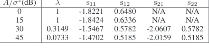
TABLE I
OPTIMAL STOCHASTIC SIGNALING. A/σ2 (dB) λ s11 s12 s21 s22 0 1 -1.8221 0.6480 N/A N/A 15 1 -1.8424 0.6336 N/A N/A 30 0.3149 -1.5467 0.5782 -2.0607 0.5782 45 0.0733 -1.4702 0.5185 -2.0159 0.5185 TABLE II
OPTIMAL DETERMINISTIC SIGNALING. A/σ2 (dB) S0 S1 0 -1.8221 0.6480 15 -1.8424 0.6336 30 -1.6911 0.7314 45 -1.6249 0.7306
In Fig. 2, the average probabilities of error are plotted versus A/σ2
for the three signaling schemes. In order to calculate both the stochastic signaling and the deterministic signaling solutions, the PSO approach is used. From Fig. 2, it is observed that for low values of σ, the conventional signaling performs worse than the others, and the stochastic signaling achieves the lowest probabilities of error. Specifi-cally, afterA/σ2
exceeds30 dB, significant improvements can be obtained via stochastic signaling over the conventional and deterministic signaling approaches. Indeed, improvements are expected based on Proposition 2 as well. For example, at30 dB,G′′(−2) = 0.6514 and G′(−2) = −0.441, and at 40 dB, G′′(−2) = 13.84 and G′(−2) = −1.389, which results in G′′
(−2) > −G′
(−2)/2 for both of the cases. Therefore, the second sufficient condition in Proposition 2 (i.e., the inequality in (19)) is satisfied and improvements over the conventional solution are guaranteed in those scenarios.
Moreover, it should be noted that the average probability of error does not monotonically decrease for the conventional and deterministic solutions asA/σ2
increases. This is because of the fact that average probability of error is related to the area under the two shifted noise PDFs as in (6). Since the noise PDF has a multimodal PDF in this example, and the amount of shifts that can be imposed on the noise PDFs is restricted by the average power constraint, that area may increase or remain same asA/σ2
increases in some cases.
In order to provide further explanations of the results, Table 1 and 2 present the solutions of the stochastic and deterministic signaling schemes for some A/σ2
values. In Table 1, the optimal s1 and s2 in (30) are expressed as s1 = [s11 s12] and s2 = [s21 s22] for each A/σ
2
value. For small A/σ2 values, such as 0 dB and 15 dB, the deterministic solutions are the same as the stochastic ones. In fact, the performance of the deterministic and the stochastic signaling is same for A/σ2
values less than 20 dB, as can be observed from Fig. 2. Also, their performance is very close to the performance of conventional signaling at highσ values. For example, at 0 dB, the average probability of error for the conventional signaling is 0.120, and it is 0.117 for the other schemes.
Furthermore, it can be observed from Table 1 that as A/σ2
increases, the randomization between two signal vectors becomes more effective and this helps reduce the average prob-ability of error as compared with the other signaling schemes. For example, at A/σ2
= 45 dB, the average probability of error for the stochastic signaling is 5.66 × 10⁻⁴
, whereas it is 0.007 and 0.02 for the deterministic signaling and the conventional signaling schemes, respectively.
V. CONCLUDINGREMARKS
The optimal stochastic signaling problem has been studied under an average power constraint. It has been shown that, under certain conditions, the conventional signaling approach, which maximizes the Euclidean distance between the signals, is the optimal signaling strategy. Also, sufficient conditions have been obtained to specify when randomization between different signal values may result in improved performance in terms of the average probability of error. In addition, the discrete structure of the optimal stochastic signals has been specified, and a global optimization technique, called PSO, has been used to solve the generic stochastic signaling prob-lem under the average power constraint. Finally, numerical examples have been presented to illustrate some applications of the theoretical results.
REFERENCES
[1] H. V. Poor, An Introduction to Signal Detection and Estimation. New York: Springer-Verlag, 1994.
[2] I. Korn, J. P. Fonseka, and S. Xing, “Optimal binary communication with nonequal probabilities,” IEEE Trans. Commun., vol. 51, no. 9, pp. 1435–1438, Sep. 2003.
[3] V. Bhatia and B. Mulgrew, “Non-parametric likelihood based channel estimator for Gaussian mixture noise,” Signal Processing, vol. 87, pp. 2569–2586, Nov. 2007.
[4] M. Azizoglu, “Convexity properties in binary detection problems,” IEEE
Trans. Inform. Theory, vol. 42, no. 4, pp. 1316–1321, July 1996.
[5] C. Goken, S. Gezici, and O. Arikan, “Stochastic signaling under second and fourth moment constraints,” in Proc. IEEE International Workshop
on Signal Processing Advances for Wireless Communications (SPAWC),
Marrakech, Morocco, June 2010.
[6] ——, “Optimal signaling and detector design for power-constrained binary communications systems over non-Gaussian channels,” IEEE
Commun. Lett., vol. 14, no. 2, pp. 100–102, Feb. 2010.
[7] A. Patel and B. Kosko, “Optimal noise benefits in Neyman-Pearson and inequality-constrained signal detection,” IEEE Trans. Sig. Processing, vol. 57, no. 5, pp. 1655–1669, May 2009.
[8] K. E. Parsopoulos and M. N. Vrahatis, Particle swarm optimization
method for constrained optimization problems. IOS Press, 2002, pp.
214–220, in Intelligent Technologies–Theory and Applications: New Trends in Intelligent Technologies.
[9] S. Shamai and S. Verdu, “Worst-case power-constrained noise for binary-input channels,” IEEE Trans. Inform. Theory, vol. 38, pp. 1494–1511, Sep. 1992.
[10] H. Chen, P. K. Varshney, S. M. Kay, and J. H. Michels, “Theory of the stochastic resonance effect in signal detection: Part I–Fixed detectors,”
IEEE Trans. Sig. Processing, vol. 55, no. 7, pp. 3172–3184, July 2007.
[11] S. Bayram, S. Gezici, and H. V. Poor, “Noise enhanced hypothesis-testing in the restricted Bayesian framework,” IEEE Trans. Sig.
Pro-cessing, vol. 58, no. 8, Aug. 2010.
[12] L. Huang and M. J. Neely, “The optimality of two prices: Maximizing revenue in a stochastic network,” in Proc. 45th Annual Allerton
Confer-ence on Commun., Control, and Computing, Monticello, IL, Sep. 2007.
[13] R. T. Rockafellar and R. J.-B. Wets, Variational Analysis. Berlin:Springer-Verlag,, 2004.
[14] D. P. Bertsekas, A. Nedic, and A. E. Ozdaglar, Convex Analysis and
Optimization. Boston, MA: Athena Specific, 2003.
[15] S. Koziel and Z. Michalewicz, “Evolutionary algorithms, homomorphous mappings, and constrained parameter optimization,” Evolutionary
Com-putation, vol. 7, no. 1, pp. 19–44, 1999.
[16] X. Hu and R. Eberhart, “Solving constrained nonlinear optimization problems with particle swarm optimization,” in Proc. Sixth World
Multiconference on Systemics, Cybernetics and Informatics 2002 (SCI
2002), Orlando, FL, 2002.
[17] K. V. Price, R. M. Storn, and J. A. Lampinen, Differential Evolution:
A Practical Approach to Global Optimization. New York: Springer,
2005.
[18] S. Bayram and S. Gezici, “Noise-enhancedM -ary hypothesis-testing in the minimax framework,” in Proc. International Conference on Signal
Processing and Commun. Systems, Omaha, Nebraska, Sep. 2009, pp.