Efficient parallel digital signal processing algorithms for hypercube-connected multicomputers

P R O C E S S E S Á L G O B iT H lá S

f ú ñ

$ У ® У ? Т Г і0 Т О Т Н Е © е ^ Д Г Г ? л Ш Т О ? С О М Ш Т іЙ

і с і ш с і

A N D П Ш т $ ш и т £ O r EN ■■ Ш Е І Ш Ш

βΦΙύ S C IE N C E

'3^<Í*Í..3!^ _{.Wird \:y.íK ■:- -wií.···«* V ν,ί*.·.} -JI í,4i¿' . . Äi _{*ь ,·\ ·.- i«},.?»,'. ·**

W ' W ¿ ί '«! ·Μ · ^ V ΜΜτ*”.

« ä Λ,-t-T-i S ■ЛИС_{w ^¿.'.»■ ^‘i ' j » · ·*' ■iiw V W W W · ' V i Ä r * . i. w · « M}

, . ГЛ !, «!< Í Л Ѵ

A fv'иГ! U ^“ÿ· /іл-іуг.? t Οΰ·!ί_{i· ,1"* Ч Ö ií '■* '·*' ‘***'}

HYPERGUBE-CONNECTED MULTICOMPUTERS

A THESIS

SUBM ITTED TO THE D EPA RTM ENT OF C O M PU T E R EN G INEERIN G A N D INFORM ATION SCIENCE AND THE IN ST IT U T E OF ENGINEERING AND SCIENCE

OF BILK EN T U NIV ERSITY

IN PARTIAL FU LFILLM EN T OF THE REQ U IR EM EN TS FO R TH E DEGREE OF

M A STER OF SCIENCE

By

Argun Derviş

April 1992

VL

^ і о г . з ■ Ь і г

1332

I certify that I have read this thesis and that in my opin­ ion it is fully adequate, in scope and in quality, as a thesis for the degree of Master of Science.

Assoc. Prof. Cevdet Ao^kanat(Principal Advisor)

I certify that I have read this thesis and that in my opin­ ion it is fully adequate, in scope and in quality, as a thesis for the degree of Master of Scienc

Assoc. Prof. Kemal Oflazer

I certify that I have read this thesis and that in my opin­ ion it is fully adequate, in scope and in quality, as a thesis for the degree of Master of Science.

Assoc. Prof. Enis Çetin

Approved by the Institute of Engineering and Science:

ABSTRACT

EFFICIENT PARALLEL DIGITAL SIGNAL PROCESSING

ALGORITHMS FOR HYPERCUBE-CONNECTED

MULTICOMPUTERS

Argun Derviş

M. S. in Computer Engineering and Information Science

Supervisor: Assoc. Prof. Cevdet Aykanat

April 1992

In this thesis, efficient parallelization of Digital Signal Processing (DSP) algorithms, (FFT, FHT and FCT), on multicomputers implementing the hy­ percube interconnection topology are investigated. The proposed algorithms, maintain perfect load-balance, minimize communication overhead, can overlap communications with computations and achieve regular computational pat­ terns. The proposed parallel algorithms are implemented on Intel’s iPS C /2^ hypercube multicomputer with 32 processors. High efficiency and almost linear speedup values are obtained for even small size problems.

Keywords: Digital Signal Processing, Hypercube, Parallel Processing, FFT, FHT, FCT.

HPSC/2 is a registered trademark of Intel Corporation

N \ N N

HIPERKUP ÇOK

BİLGİSAYARLARINDA

v e r i m l i p a r a l e l

SAYISAL İŞARET İŞLEME

ALGORİTMALARI

Argun Derviş

Bilgisayar Mühendisliği ve Enformatik Bilimleri Bölümü

Yüksek Lisans

Tez Yöneticisi: Assoc. Prof. Cevdet Aykanat

Nisan 1992

Bu tez kapsamında, hiperküp bağlantı yapisini içeren çok işlemcili bilgisa­ yarlarda, tek boyutlu Sayisal İşaret İşleme algoritmalari, FFT, FHT ve FCT araştirilmiştir. Önerilen algoritmalar, eşit yük dağilimi, minimum haberleşme, haberleşmeleri sayisal işlemlerle birleştirebilme ve düzgün algoritmik yapilar içermektedir. Önerilen paralel algoritmalar, Intel’in hiperküp bilgisayarinda, 32 işlemcisiyle denenmiştir. Küçük boyuttaki problemler için bile yüksek kazanç ve hizlar elde edilmiştir.

Anahtar kelimeler : Sa5Üsal işaret işleme, Hiperküp, Paralel işleme, FFT, FHT, FCT.

ACKNOWLEDGEMENT

I would like to express my deepest gratitude to Assoc. Prof. Dr. Cevdet Aykanat for his guidance, suggestions, advice, encouragement and his friendly supervision. I shall always be indebted to ASELSAN Military Electronics Inc. and the manager of Embedded Systems Division İsmet Atalar for the consid­ erable support that, they have provided to me during my study.

I am also gratefull, to Assoc. Prof. Dr. Kemal Oflazer and Assoc. Prof. Dr. Enis Çetin for their valuable suggestions. I would also like to thank to my friends especially to Taçli Yazicioğlu and Ayşegül Göçmen for their endless support and morale.

I finally would like to thank to my family for their endless support and kindness that they have provided to me.

1 Introduction 1

2 The Fast Fourier Transform 5

2.1 Intro d u ctio n ... 5

2.2 The Sequential FFT A lg o r ith m ... 6

2.3 Parallel FFT A lgorithm s... 9

2.3.1 Perfect Load B a la n ce ... 13

2.3.2 Overlapping Communication with C o m p u ta tio n ... 18

2.4 Experimental R e su lts... 25

2.5 Conclusion... 30

3 T he Fast H artley Transform 32 3.1 In tro d u ctio n ... 32 3.2 Sequential FHT A lg o rith m ... 33 3.3 Parallel FHT A lg o r ith m ... 43 3.3.1 Perfect Load B a la n ce ... 48 3.4 Experimental R e s u lts ... 67 VI

CONTENTS Vll

3.5 Conclusion 68

4 The Fast Cosine Transform 71

4.1 In tro d u ctio n ... 71

4.2 Sequential FCT A lg o rith m s ... 72

4.2.1 Lee’s Sequential FCT A lgorithm ... 73

4.2.2 Malvar’s Sequential FCT A lgorithm ... 75

4.3 Perfect Load Balance FCT A lgorithm ... 78

4.4 Experimental R e su lts... 82

4.5 Conclusion... 84

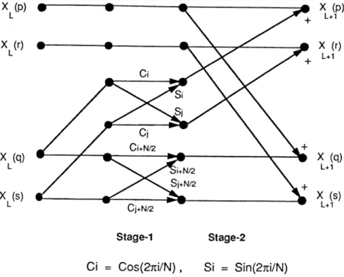
2.1 Simplified Butterfly. 7

2.2 Basic Butterfly... 7

2.3 Computational flow graph for a 16-point FFT and its static map­ ping on an hypercube with 4-processors... 11

2.4 Dynamic mapping of 16-point FFT data and computations on a hypercube with 4-processors... 15

2.5 Variation in a with respect to N /2 P ... 17

2.6 Percent Overlap curve for Program (2.4) compared to Program(2.3). 26 2.7 Percent Overlap curve for Program (2.5) compared to Program (2.3). 27 2.8 Percent Improvement of Program (2.3) over Program (2.2) dur­ ing the last d-stages... 28

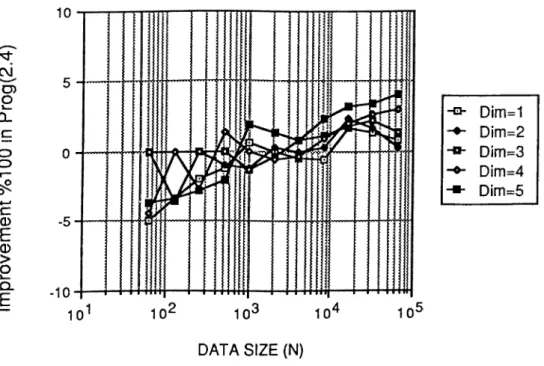
2.9 Percent Improvement of Program (2.4) over Program (2.3) dur­ ing the last d-stages... 28

2.10 Percent Improvement of Program (2.5) over Program (2.3) dur­ ing the last d-stages... 29

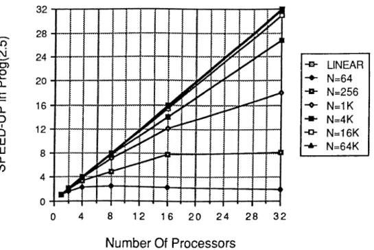
2.11 Speedup curve for Program (2.5)... 29

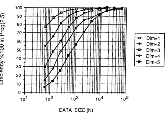
2.12 Efficiency curve for Program (2.5)...30

3.1 Computational steps in Fast Hartley T ra n sfo rm ... 35

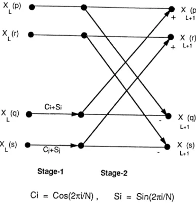
3.2 Basic Fast Hartley Transform Butterfly, Typel (1 < ^ < n-1) . . 36 3.3 Basic Fast Hartley Transform Butterfly, Type2 ( ! < ^ < n - l ) . . 36 3.4 Simplified Fast Hartley Transform Butterfly, T y p e l ...38 3.5 Simplified Fast Hartley Transform Butterfly, Type2 ...39 3.6 Sequential FlowGraph of Fast Hartley Transform for N=32 points 40 3.7 Static mapping of an (N=32) point Fast Hartley Transform on

a 3-dimensional h y p e rc u b e ... 45 3.8 Two steps of Simplified Fast Hartley Transform Butterfly, Typel 50 3.9 Two steps of Simplified Fast Hartley Transform Butterfly, Type2 51 3.10 Two steps of Restructured Simplified Fast Hartley Transform

Butterfly, T y p e l... 55 3.11 Two steps of Restructured Simplified Fast Hartley Transform

Butterfly, T y p e2 ... 56 3.12 Restructured Fast Hartley Transform for N=32 p o in ts ...58 3.13 Static Mapping of Restructured Fast Hartley Transform for N=32

points on a 2-dimensional h y p e rc u b e ... 63 3.14 Dynamic Mapping of Fast Hartley Transform for N=32 points

on a 4-node h y p e rc u b e ... 65 3.15 Speedup curve for Prog.(3.3)...69 3.16 Efficiency curve for Prog.(3.3)... 69

4.1 Computational Flow Graph of 16-point FCT (Lee’s method). . . 73 4.2 Basic FCT B u t te r f ly ... 76 4.3 Computational Flow Graph of 16-point FCT (Malvar’s method). 77

4.4 Dynamic mapping of 32-point FCT on a 4-processor hypercube (Malvar’s method)... 80 4.5 Speedup curve for Prog. (4.3)... 83 4.6 Efficiency curve for Prog. (4.3)... 84

List o f T ables

3.1 Sequential timing results of F F T and F H T , Prog.(2.1) and Prog.(3.1) (msec)... 53

4.1 Timing results (msec) for sequential FCT algorithms, Prog. (4.1) and Prog. (4.2). . ... 33

In the 1960s, a group of engineers and mathematicians working at AT&T Bell Labs invented a set of techniques known as Digital Signal Processing (DSP). The algorithms they invented are used today in many fields, including radar, sonar, seismic processing, image enhancement, communications, radio astron­ omy, medical imaging and etc.

Digital Signal Processing of real-time signals has gained importance with re­

cent advances in digital computer technology. Digital signal processors - digital computers specializing in signal processing - are in development and available on the market. All of this growth is for massive amounts of computations in various DSP applications.

One way to satisfy the performance requirement of DSP applications is to choose clever algorithms or expand the processor performance or both of them. DSP applications are characterized by computations that are massive but fairly straightforward and simple. Furthermore, these computations exhibit orderly structures. Besides, DSP algorithms are very efficient. These algorithms are optimized and improved several times until now. However, it is still not enough for most of the DSP applications. Performance of conventional computers are still very limited in cases where extensive number crunching computations are required. Discrete Fourier Transform (DFT), Discrete Hartley Transform (DHT) and Discrete Cosine Transform (DCT) are such examples.

Discrete Fourier Transform provides an efficient method for spectral anal­

ysis of discrete signals. Thus, Cooley and Tukey providing a more efficient algorithm [1], named as Fast Fourier Transform (FFT), made possible many applications concerning the computation of DFT to be realizable because of performance problems. FFT algorithm hcis a very wide application domain and known to be the most widely used digital signal processing transformation.

Beyond the highly accepted usage of FFT, it is a complex transforma­ tion. If the signals in the time domain are real, then the FFT contains redun­ dancy. Discrete Hartley Transform (DHT) exists for this reason [11] and can be called as a real version of DFT. Discrete H artley T ra n sfo rm is applied to signals, where the domain is formed of only real inputs. As well as FFT,

Discrete H artley T ra n sfo rm has also a fast formulation called Fast Hartley T ra n sfo rm FHT [13]. FHT provides efficient spectral analysis of real discrete

signals and it is faster than FFT.

Dicrete Cosine T ra n sfo rm (DCT) [20] is another transformation for DSP.

DCT is used mainly for speech and image coding applications. DCT is also a real transformation like DHT and has also a fast computation formula referred as Fast Cosine T ra n sfo rm [25] or shortly FCT in this work. Importance of FCT comes from the fact that, it has the best performance among the other known fast computable transforms. With this feature FCT is a promising al­ ternative to FFT and FHT.

CHAPTER 1. INTRODUCTION 2

As mentioned earlier, although fast algorithms exist for DSP transforma­ tions, conventional computers are still not fast enough to compute these al­ gorithms (FFT, FHT, FCT) in real-time. Extensive research has been made in this area, in order to overcome the difficulties faced during real-time com­ putation of DSP algorithms. This led people to design special purpose hard­ wares, DSP microprocessors, VLSI circuits and use general high-performance computers to solve these problems in real-time. Distributed memory, message­ passing parallel computers, which are usually named as multicomputers, are

the most promising general purpose high performance computers. These ar­ chitectures have the nice scalability feature due to the lack of shared resources and increasing communication bandwidth with the increasing number of pro­ cessors. In multicomputers, processors have neither shared memory nor shared address space. Each processor can only access its local memory. Processors of a multicomputer are usually connected by utilizing one of the well-known direct interconnection network topologies such as ring, mesh, hypercube and etc. Hypercube topology is very well suited for many of the DSP applications including FFT, FHT and FCT.

In this thesis, efficient parallelization of several one-dimensional FFT, FHT and F C T algorithms on multicomputers implementing the hypercube inter­ connection topology are investigated. In order to achieve speedup on such architectures, the algorithm must be designed so that both computations and data can be distributed to the processors with local memories in such a way that computational tcisks can be run in parallel, balancing the computational loads of the processors. Communication between processors to exchange data must also be considered as part of the algorithm. One important factor in designing parallel algorithms is granularity. Granularity depends on both the application and the parallel machine. In a parallel machine with high com­ munication latency, the algorithm should be structured so that large amounts of computation are done between successive communication steps. Another im portant factor is the ability of the parallel system to overlap communication and computation. In order to exploit this property of the parallel system, the algorithm must be structured so that the communication can be overlapped with computation. The algorithms presented in the following chapters, achieve efficient parallelization by considering all these points in designing efficient parallel one dimensional FFT, FH T and FC T algorithms for hypercube multi­ computers. These parallel algorithms eliminate fragmentary message passing for efficient parallelization on medium-to-coarse grain, MIMD type hypercube multicomputers. Proposed parallel algorithms do not disturb the inherent reg­ ularity of FFT, FHT and FCT so that they can be implemented on SIMD type hypercube multicomputers. These algorithms are structured such that over­ lapping communications with computations is possible. Proposed algorithms

are written and compiled in ANSI C language on a 32-node iPSC/2 hypercube multicomputer.

CHAPTER 1. INTRODUCTION 4

In chapter 2.3.1, perfect-load balance FFT algorithm is discussed. In chap­ ter 2.3.2, overlapping FFT algorithms are presented. In chapter 2.4, experi­ mental results are given for the presented algorithms.

In chapter 3.3.1, restructuring of FHT along with its perfect-load balance algorithm is presented. In chapter 3.4, experimental results are given for the presented algorithms.

In chapter 4.2.2, parallelization of FCT along with its relation to FHT is presented. In chapter 4.3, perfect-load balance FCT algorithm is given. In chapter 4.4, experimental results are given for the presented algorithms.

2.1

In tro d u ctio n

After its’ foundation in the Century by Jean Baptiste Joseph Fourier, Discrete Fourier Transform (DFT) has been the most widely used signal pro­ cessing transform all over the world. It simply transforms signals from their time domain to their frequency domain; in other words, obtains the frequency components of a signal.

Discrete Fourier Transform is the heart of digital signal processing appli­ cations and used in most of the digital signal processing applications. Some include cellular-phones, radar, sonar, satellite communications, VCRs, hi-fi equipment, camcorders etc.. Also other DSP transforms can also be computed with the help of DFT.

The Discrete Fourier Transform of a signal f{ i) (e = 0 ,1, . . . , — 1) is,

m = E f ( i ) K ‘ i=0 N - l = 53(/(0[C'os(27ribi7iV)-i5m(27rH/A^)]) (2.1) 1=0 where (k= 0, l , . . . , N-l) and

As is written, DFT requires on the order of multiplications and addi­ tions. If is a power of 2, (eg., N — 2”) then there are several ways to change

this Fourier Transform into something different called Fast Fourier Transform (FFT) which can be calculated in less time [1]. The difference between DFT and FFT is the computation methods.

Different strategies exist for the computation of FFT and some include deci­ mation in-time, decimation in-frequency, radix-2, radix-4, radix-8, mixed-radix etc. Some algorithms are named after their founders such as Cooley-Tukey FFT [1], Good-Thomas FFT [2], Goertzel FFT [4], Winograd FFT [3] etc.

The FFTscheme choosen for parallelization is Radix-2 Cooley-Tukey scheme and the sequential algorithm is presented and discussed in Section 2.2. Paral­ lelization of the chosen FFT scheme is discussed in Section 2.3. Parallel FFT algorithms presented in Section 2.3 are implemented on an 32-node iPSC/2 hy­ percube multicomputer. Section 2.4 presents the implementation results and the relative experimental performance evaluation of the designed algorithms.

2.2

T h e S eq u en tial F F T A lg o rith m

CHAPTER 2. THE FAST FOURIER TRANSFORM 6

There are many variants of the F F T algorithm in the literature [5]. The

decimation-in-time decomposition scheme, with input in bit-retiersed order, is

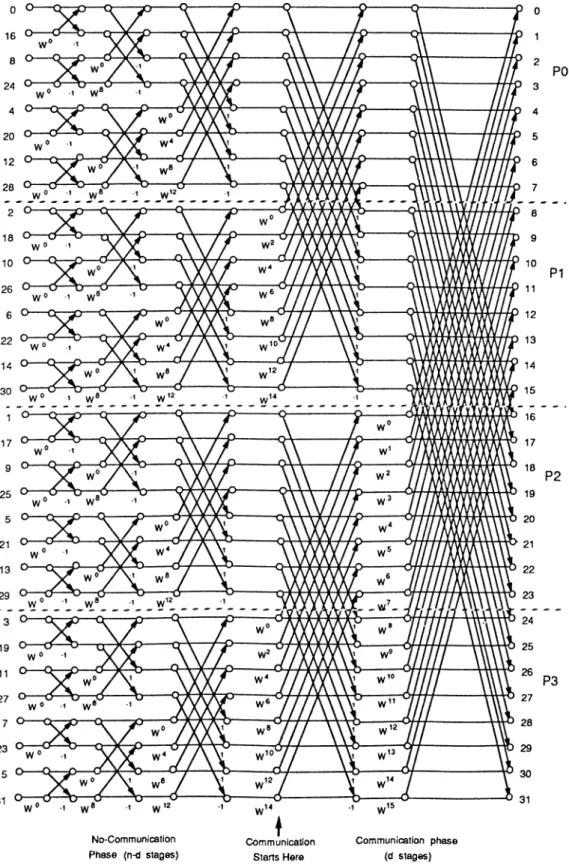
investigated in this chapter. The computational flow graph of this scheme is given in Figure 2.3 for a (N=16)-point FFT computation. The input in this scheme is iV-complex numbers in bit-reversed order. The output is A-complex numbers in normal order. As is seen in Figure 2.3, each stage of the compu­ tation takes a set of N complex numbers and transforms them into another

N complex numbers. This process is repeated n = logj N times, resulting

in the computation of the desired discrete Fourier transform in normal order. At each stage of the FFT algorithm N /2 simplified-butterfly computations are performed. The computational flow graph for simplified-butterfly computation is illustrated in Figure 2.1. On the other hand, in the basic-butterfly scheme two complex multiplications and two additions/subtractions are performed on each F F T point. Fig. 2.2 shows clearly the redundant multiplication which is

X (P) k

X,(q) k

Figure 2.1. Simplified Butterfly.

X (p) k

X ,(q) k

Figure 2.2. Basic Butterfly, discarded in the siinplified-buitci'fly scheme.

The simplified-butterfly computations required at the stage of an N- point FFT algorithm is,

temp = W]^ X Xk{q)

^k+i{p) = Xk{p) + temp

^^k+i{q) = X k { p ) - te m p (2.2)

where q = p -l· 2^', Wjij = That is, at the stage, N /2

simplified-butterfly computations are performed on partially transformed pairs separated

The SEQFFTk function shown in this program performs N /2 simplified-

butterfly computations required at the k^'’· stage of the algorithm. The SF- QFFTk function is invoked n = log2 N times to compute the complete A^-point FFT. In this program, A^-complex inputs a.o(f) {i = 0 , 1, . . . , 1) are assumed to be stored, in bit-reversed order, in one dimensional A'-array of size N. Note that, after the initialization of input in the Al-array, the computations are per­ formed in place and the results are obtained in the A^-array in normal order [5].

CHAPTER 2. THE FAST FOURIER TRANSFORM 8

As is seen in Eq. 2.2 and Prog. 2.1 only one complex multiplication and two complex addition/subtraction operations are required in a butterfly computa­ tion. Since N /2 butterfly computations are performed at each stage, the FFT algorithm requires (A/^/2) log2 A^ complex multiplications and 7Vlog2 A'^ com­ plex additions and subtractions. Hence, the calculation of an A^-point FFT requires 2A^log2 N real multiplications and 3A^log2 N real additions. Since the real multiplication and addition takes almost equal amount of time in most of the current arithmetic coprocessors (e.g., 80387[6]), the complexity of the sequential F F T can be expressed as,

= [5iVlog2yV]ica/c (2.3) where tcaic ¡s tlie time taken by a floating point multiplication/addition.

The computations of the complex coefficients M'7/ are not involved in the given complexity analysis. In most of the real time applications (e.g., radar applications), A^-point FFT is applied consecutively, for a fixed N , to A^-point input data sets. Hence, the computation of the W fa c coefficient values (twiddle factors) as they are needed, will be extremely inefficient. Hence, in general, N /2 coefficient values are computed once, as the value of the N is fixed, and stored in a table. These coefficients are then accessed by a simple table lookup procedure during successive F FT computations. Thus, the computational complexity of the coefficient calculations are negligible in such applications.

/* Input in bit-reversed order in X[0 ... N-1] */ /*' Output in normal order in X[0 . . . N-1] */

n := logj N

for k :=0 to n — 1 do

C all SEQFFTk (X, Wfac, N, k) en d fo r

/* Performs N/2 Butterfly computations over the bit */

SEQFFTk (X,Wfac,N,k) for i :=0 to {N12^'^^) — 1 do for j :=0 to 2^ — 1 do p := i X 2'^'+’ -t- j q := P + 2*-· temp := Wfac x X(q) X(q) := X(p) — temp X(p) := X(p) + temp endfor en d fo r en d SEQFFTk P ro g ra m 2.1 : Sequential N-pt FFT Algorithm

2.3

P arallel F F T A lg o rith m s

Butterfly computation of the FFT algorithm is very suitable for parallelization on multicomputers implementing the hypercube interconnection topology. The distribution of data and computations is straightforward for coarse grain par­ allelism whenever the number of F F T points, N = 2", is greater than or equal to the number of processors, P — 2^, in the hypercube. The straightforward mapping can easily be achieved by using the decimal ordering of the processors in the hypercube. The first processor in the decimal ordering is assigned the first M = N fP points of the A-array, the second processor will be assigned the next M-points and so on. Hence, successive processors in the decimal ordering will be assigned the successive slices of the X-array with each slice containing equal amount of, M = N /P , F F T points. The decomposition of a 16-point

F F T data and computations on a 2-dimensional hypercube, with M = 4 FFT

points assigned to each processor, is illustrated in Figure 2.3. In this scheme, each processor is responsible for carrying out the complete in place computa­ tions required for the FFT-points assigned to itself. As is seen in Figure 2.3, in

CHAPTER 2. THE FAST FOURIER TRANSFORM 10

the first {n — d) stages of the FFT algorithm butterfly computations are per­ formed for pairs separated by 2“, 2^,... Hence, no communication is required between processors during the first (n — d) stages since butterfly pairs separated by up to M /2 = N f2 P = 2”'/(2*2'^) = are assigned in groups to the same individual processors. In the last d stages of the FFT algorithm, butterfly pairs are separated by 2”“'^, 2"“'^"''\. . . , 2”“ ’ where p and q points of each butterfly pair are assigned to different neighbor processors whose indices differ by 2 ° , 2 \ . . . ,2“^-^ respectively. Hence, ¿-concurrent exchange commu­ nication steps are required in the last d stages of the parallel F F T algorithm where d = logj P- A pseudo-code for the node program of the parallel FFT algorithm is given in Prog. 2.2.

The function SEQFFTk given in Prog. 2.1 performs the in place (in X - array) computations corresponding to the stage of an A/^-point FFT. The first for-loop in Prog. 2.2 accumulates the summations over the first (n — d) bits by performing butterfly computations for the local p, q pairs separated by 2°, 2 \ 2 ^ , . . . , 2”““^“ ^ Hence, the first for-loop involves no interprocessor communication. The second for-loop in Prog. 2.2 accumulates the summa­ tions over the last ¿-bits by performing butterfly computations for the p, q pairs separated by 2"““^, 2""'^'*·^,..., 2”~^. Hence, an A^-point data exchange is performed concurrently at each iteration of the second for-loop by issuing a send/receive message pair. As is seen in Prog. 2.2, this scheme introduces a storage overhead of size N /P per processor due to the local receive buffer

XRB-axToy.

The straightforward mapping scheme described above achieves mapping the FFT-poiut groups that need mutual communication into nearest-neighbor processors of the hypercube. However, this scheme hcis two major drawbacks. First, in the given scheme, partially transformed N /P FFT-points have to be exchгınged between pairs of processors at each stage of the last d stages. Second, perfect load balance is disturbed during the last d stages. These two drawbacks can explicitly be seen when Prog. 2.2 is analyzed. At each iteration of the second for-loop., one half of the processors hold only the updated values

No-Comm unication Phase (n-d stages)

Com m unication Starts Hero

Com m unication phase (d stages)

Figure 2.3. Computational flow graph for a 16-point FFT and its static map­ ping on an hypercube with 4-processors.

CHAPTER 2. THE FAST FOURIER TRANSFORM 12

/* Computation over the first (n — d) bits: No communication */

n := logj N] d := logj P; M := N /P] m := ]og2 M;

for k :=0 to n — d — 1 do Call SEQFFTk (X,Wfac,M,k) endfor

/* Computation over the next; hence the last d bits */

/* d concurrent exchange steps */

for k :=n — d to n — 1 do

£ — k — (n — d); dnode := mynode © 2^;

if ((P* bit of mynode) = 1) then do for i :=0 to M — } do

X(i) : = Wfac X X(i) endfor

csend from (X(i): i= 0,l,2, . . . , M-1) to dnode crecv into (XRB(i): i=0,l,2, . . . , M-1) from dnode for i :=0 to M — 1 do

X(i) := XRB(i) - X(i)

endfor else

csend from (X(i): i= 0,l,2, . . . , M-1) to dnode crecv into (XRB(i): i=0,l,2, . . . , M-1) from dnode for i :=0 to M — 1 do

X(i) := X(i) © XRB(i)

endfor endif endfor

Program 2.2 : Parallel N-pt FFT Algorithm on a hypercube with P proces­

sors

for the p-points and the other half hold only the updated values for ^-points of the butterfly pairs. Since only the updated values of the ^-points of the butterfly pairs have to be multiplied by the coefficients those processors holding

N jP q-points performs N /P complex multiplications and the other processors

waits idle for receiving the multiplication results from those processors. Hence, the parallel complexity of this scheme is,

57V N RN N

Tp2 = [-p-^Og2^]tcalc+[-p-iog2P]tcalc-I-[tau + -pttr]^Og2P (2.4)

Here, fju represents the message startup overhead or the message latency and

tir is the time taken for the transmission of a complex floating-point word

(2 4 bytes) between two neighbor processors. Note that, the performance of the given scheme effectively degrades to the performance of the basic-butterfly

scheme (two complex multiplications per pair) during the last d stages. The communication time required for down-loading the input data and off-loading the results to/from the processors of the hypercube is not included in the above complexity model. However, each one of these operations can be performed in logj P communication steps.

2.3.1

P erfect Load B alan ce

Parallel E F T algorithms which achieve perfect-load balance are given in [7] for input in bit-reversed order and in [8] for input in normal order. Both of these two parallel algorithms exploit the simplified-butterfly scheme. The implementation details are not given explicitly in [8]. The parallel running time model given in [8] shows the volume of comunication as N /P complex

F F T points per stage although it is indicated that only N /2 P complex FFT

points are exchanged in a stage. The parallel program implemented in [7] performs two exchange communications per stage of the FFT algorithm. The algorithms given in [9] also achieve perfect load balance. However, these algo­ rithms use basic-butterfly scheme iov the FFT computations. In this subsection, we present a parallel FFT algorithm which achieves perfect load-balance for the F F T scheme using the simplified-butterfly with inputs in bit-reversed order. In the presented scheme, N /2 P complex FFT points are exchanged only once between processor pairs at each stage of the last d-stages.

The straightforward mapping scheme used in Prog. 2.2 already maintains perfect load balance during the first (n — d) stages. Hence, this mapping is maintained during the first (n — d) stages of the parallel algorithm proposed in this subsection. As is indicated earlier, one half of the processors hold only updated values for the p-points and the other half hold only the updated val­ ues for the ^-points of the butterfly pairs during the last d-stages. This static mapping scheme is altered at the beginning of each stage of the last d stages. At the very beginning of each stage, each processor holding only updated val­ ues for the ^-points [N /2P FFT points) exchange one half of its ^-points with the N ¡2P p-points of its neighbor processor which holds all the p-points of its

CH A PTER 2. THE FAST FO URIER TRA NSFORM 14

butterfly pairs of that stage of the algorithm and vice versa. This exchange operation is not only the échangé of data values to be used at that stage of the algorithm. In fact, processors effectively exchange the responsibility of the further F F T computations associated v^dth those exchanged F FT points.

This dynamic mapping scheme is illustrated in Figure 2.4 for a 16-point

F F T on a 4-processor hypercube. The pseude-code for the node-program of

the proposed parallel FFT algoithm is given in Prog. 2.3. A C-like notation is used in Prog. 2.3 and throughout the chapter to represent the for-loops. The initial mapping scheme and the first for-loop in Prog. 2.3 is exactly similar to Prog. 2.2. It is the second for-loop where those two programs differ from each other. As is seen in Figure 2.4 and Prog. 2.3, each processor exchange either the first half or the second half of its local A^-array in place by simply checking the bit value of its processor index where I denotes the channel over which the exchange operation is to be performed on that stage. Due to the dynamic mapping scheme, each processor performs ÿimplified butterfly computations on local p and q pairs separated by 2”‘^~^ = N j2 P after the exchange operations at each stage of the last d stages. Hence, in this scheme, each processor holds equal number of p and q points {N f2P p-points and N /2 P q-points) after the exchange operation. Each processor performs equal number of (N /2P ) com­ plex multiplication thus achieving a perfect load balance. Furthermore, the volume of communication at each exchange communication step is reduced by a factor of two (from N /P to N f2 P complex floating-point words). Hence, the parallel complexity of the proposed scheme is.

P

N N

T p 3 — [ u ^ ] l c a l c “t" [^su T ^ "f (^•'^)

In the complexity model given above, two concurrent serid communication op­ erations (for an exchange operation) between a pair of processor are assumed to be overlapped completely. The startup overheads (<,„) for the mutual semd operations are in fact overlapped completely. The overlap of mutual data trans­

27 O—t f S ?

31

o ( / \ Q X r ^ / A/

X t) -- O--- O-A A A O______

/V w* /YY\ ---- Q- /Y \^ —o— o X X _{w'* /VYV} M / V \ r W ® .1 J / V V w'® / / \ V w’* / / \ V V w " / \ W® -I W * ·’ No-CommunIcation ‘ w” ’ 1 ° w” ■’

Communication Communication phase

w’* ·'

Phase (n-d stages) Starts Here (d stages)

Figure 2.4. Dynamic mapping of 16-point FFT data and computations on a hypercube with 4-processors.

CHAPTER 2. THE FAST FOURIER TRANSFORM 16

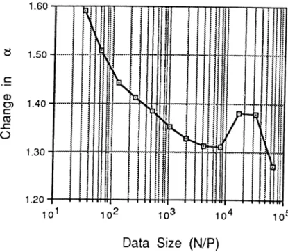
links are present between neighbor processors as in iPS C /2. However, the in­ ternal hardware architecture of an individual iPSC/2 processor is such that internal bus conflicts occur due to the outgoing and incoming long messages during an exchange operation. Hence, a complete overlap cannot be achieved in iPSC/2 during the mutual data transmission Y>ha.se of the exchange operation. The performance of the exchange operation can be modeled as [tsu - f a x -^ttr] in iPSC /2, where a is measured to be 1.3 < a < 1.6 in [10]. The variation of

a with respect to concurrent incoming and outgoing message length is given

in Figure 2.5. Hence, this a parameter should be inserted as a coeflScient to the term in Eq. 2.5 to give the running time model of the parallel algo­ rithm on iPSC/2. Note that, in Prog. 2.3, each processor issues synchronous

receive just after the synchronous send operation. Due to the perfect load

balance, communicating processor pairs perform the synchronous send opera­ tions concurrently. A synchronous send operation returns the control back to node program only after the outgoing message leaves the indicated send buffer A"6'j9-array. Whenever an incoming message begins to arrive to a destination processor, it does not find a pending receive, hence it is copied to a temporary system buffer by the node operating system NX. Later, whenever the receive operation is issued by the node program, that message is copied from the tem­ porary system buffer to the indicated receive buffer X-array. Hence, late issue of the synchronous receive message introduces a block copy overhead for N ¡2P complex floating-point words. The last term in Eq. 2.5 accounts for this receive overhead where t^opy represents the time taken for the copy of a single complex floating-point word from the system buffer to the indicated receive buffer X - array. Note that, such a receive overhead is not included in the parallel time complexity model given in Eq. 2.4 for Prog. 2.2. In Prog. 2.2, due to the lack of load balance, communicating processor pairs do not initiate send operations concurrently. The model in Eq. 2.4 is given for the bottleneck processors which stay idle, waiting for the multiplication results from their neighbor processors. These processors always issue an early synchronous receive. Due to a pending receive for an incoming message, the incoming message is directly copied into the indicated receive buffer X /?jB-array.

Figure 2.5. Variation in a· with respect to N /2P .

/* Computation over the first (??. — d — 1) bits: No communication */

n := logj/^; d := log-2 P; M := A^/P; m := log2 M\

for k :=0 to n — d — 1 do

Call SEQFFTk (X, Wfac, M, k)

endfor

I* Computation over the next d bits: d concurrent exchange steps */

for k :=n — d to n — 1 do

£ := k — (n — d)] dnode := mjmode 0 2^; if ((P^' bit of mynode) = 1) th e n do

csend from (X(p): p=0,l,2, . . . , M/2 — 1) to dnode crecv into (X(q): q=0,l,2, . . . , M/2 — 1) from dnode else

csend from (X(q): q = M /2, M /'l — 1, M /2 — — 1) to dnode

crecv into (X(p): p = M /2, M /2 — 1, A//2 — 2 . . . , M — 1) from dnode endif for (p :=0, q \=M¡2\ p < A //2; p + + , q+ P ) do temp := Wfac x X(q) X(q) := X(p) - temp X(p) := X(p) + temp endfor endfor

P ro g ra m 2.3 : Parallel N-pt FFT Algorithm with Perfect Load-Balance on a hypercube with P processors

CH A PTER 2. THE FA ST FO URÎER TRA NSFORM 18

balance. As is seen in Prog. 2.3, this scheme requires no extra storage for

send!receive buffers since send/receive operations are performed in place to

or from the local A"-array. As is seen in Figure 2.4, the output results are slightly scrambled (in N /2 P blocks) in this scheme due to the dynamic map­ ping scheme proposed. However, the off-loading of the results from the pro­ cessors of the hypercube can also be performed in log2 P communication steps without increasing the volume of communication.

2.3.2

O verlapping C o m m u n ication w ith C o m p u ta tio n

There are strong data dependencies in the FFT algorithm. The update of each FF T point requires communication in tlie last d-stages of the algorithm. Hence, as is also indicated in [9, 10], the F F T algorithm differs from local spatially decomposed problems such as Finite Difference and Finite Element problems. In such problems, communications associated with the boundary points can easily be overlapped with the updating of interior data points[9j. Thus, com­ munication and computation in the FFT algorithm cannot be overlapped easily.

Zhu has proposed a scheme for overlapping communication with the com­ putation of the complex coefficients (complex exponentiations) in [8]. However, as is discussed earlier, computation of the coefficients as they are needed is not an efficient scheme compared to the table lookup scheme. Walker has proposed a scheme in [9] for overlapping communication and computation for the F FT algorithm using the basic-butterfly scheme which requires two complex multipli­ cation per butterfly pair. In this section, we propose two schemes which overlap the communication with one fifth of the computations involved in a stage of the FjET algorithm which uses the simplified-butterfly and the table lookup scheme.

Schem e 1: A synchronous Send and Synchronous R eceive

The pseudo-code for the node program of the parallel F F T algorithm which overlaps communication and computation is given in Prog. 2.4. The initial

static mapping for the first (n — d) stages and the dynamic mapping for the

last d-stages is similar to the scheme given in Prog. 2.3. However, as is seen in Prog. 2.4, the first for-loop iterates only (n — d — 1) times which is one less than the iteration count in Prog. 2.3. Then at each iteration (computation stage) of the second for-loop each processor pipelines the send portion of the exchange operation required at the following stage in the current stage. Each processor classifies its computational task at each stage into two categories: those updates to be sent to the destination processor in the following stage and other updates to be kept as local in the following stage. Then, each pro­ cessor first performs the computations associated with those points required by the destination processor in the next stage. Hence, each processor first per­ forms N /2P complex multiplications associated with its local N /2 P q-points. Then, each processor updates either the values of its local p-points or ^-points simply by checking the (£ bit value of its processor index. Here, ^ + 1 denotes the channel over which the exchange operation required in the next stage. Upon completion of these N /2 P updates, each processor issues an asyn­

chronous (non-blocking) send to initiate the transmission of the updated N /2P

FFT-point values to the destination processor. After initiating the send oper­ ation, each processor completes the computation associated with that stage by updating other half of its local FFT-points that will be kept local in the follow­ ing stage. Upon completion of the second type updates each processor issues a synchronous receive to complete the already initiated exchange operation.

As is seen in Prog. 2.4, the first inner for-loop of the second outer for-loop performs the updates to be send immediately to the destination processor. Each processor performs these updates into a send buffer {XSB array) of size

Nf 2 P since it does not need these updates in further FFT computations. How­

ever, receive portion of the exchange operations can be done in place into the local A-array since synchronous receive is issued after the completion of the overall computations associated with that stage. Hence, the proposed scheme

CHAPTER 2. THE FAST FOURIER TRANSFORM 20

/* Computation over the first (n — d — 1) bits: No communication */ n r^ lo g jA ^ ; d := lo g 2P; M : = N / P · , m := ] o g 2 M;

for k :=0 to n — d — 2 do

Call SEQFFTk (X, Wfac, M, k) endfor

/* Computation over the next d bits: d-concurrent exchange comm, steps */

for k :—n — d — 1 to n — 2 do

£:= k — {n — d); dnode := mynode 0 2^+^;

if {{£ + bit of mynode) = 1) then do

for (p :=0, q :=Ai/2; p < A//2; p + + , q 0 + ) do X(q) := Wfac x X(q)

XSB(p) X(p) + X(q)

endfor

isend from (XSB(p): p = 0 ,1 , 2 , . . . , M /2 — 1) to dnode

for (p := 0, q :=M/2; p < M/2; p + + , q++) do X(q) := X(p) - X(q)

endfor

crecv into (X(p): P = 0 ,1 ,2 ,..., M /2 — 1) from dnode else

for (p :=0, q :=M /2; p < M /2; p + + , q + + ) do

X(q) := Wfac X X(q) XSB(p) := X(p) - X(q)

endfor

isend from (XSB(q): q = 0 , 1 , 2 , . . . , A//2 — 1) to dnode for (p :=0, q :=Mf2·, p < M/2; p + + , q+ + ) do

X(p) := X(p) + X(q) endfor

crecv into (X(q): q = M /2, M /2 -f M /2 + 2 . . . , M — 1) from dnode

endif

m sgw ait on isend endfor

/* Perform M /2 Butterfly computations over the local (m — 1)*^‘ bit */

Call SEQFFTk (X, Wfac, M, m - 1)

P ro g ra m 2.4 : Overlapped Parallel N-pt FFT Algorithm with Perfect Load- Balance on a hypercube with P processors Scheme

introduces a storage overhead of size N / 2 P per processor due to the local send buffer XSB array. Note that, the size of the local A’-array is N / P . The only computational overhead is the loop overhead since two for-loops are required instead of one. The number of floating-point computations is exactly equal to the number of computations required in Prog. 2.3. As is seen in Prog. 2.4,

N / 2 P complex additions/subtractions shown in the second inner for-loop of

the second outer for-loop are overlapped with communication. Hence, commu­ nication is overlapped with one fifth of the computations involved in a stage. Thus, the parallel complexity of the proposed algorithm is

I)N N AN

Tp4 [ p ~p\lcalc “t" [ p log2 P]tcalc T

N N N

[ Mq.x{ p i c a t c i Usu T ^ ’P

2P '■copy

Hence, for sufficiently large N f P^ where.

N N

plcalc ^ l-su T 2,P^^^

complete overlap of communication can be achieved.

(

.

)

(2.7)

Schem e 2: Asynchronous Send and Asynchronous R eceive

As is seen in Prog. 2.4, only the send portion of the communication is over­ lapped with one fifth of the computation. Note that, in Prog. 2.4, each pro­ cessor issues synchronous receive after initiating asynchronous send operation and performing N / 2 P complex addition/subtraction operations. Due to the perfect load balance, communicating processor pairs initiate the asynchronous

send operations concurrently. Hence, there is no pending receive in a destina­

tion processor for an incoming message. The last term in Eq. 2.6 accounts for the receive overhead due to the late issue of the synchronous receive operation. If, however, there is a pending asynchronous receive for an incoming message, then it is directly copied into the indicated receive buffer. Hence, it is also pos­ sible to overlap the receive portion by issuing an early asynchronous receive. In this section, we present a second scheme which overlaps both send/receive portions of the communication with computation using the simplified-butterfly and the table lookup methods described before. The pseudo-code for the node

CHAPTER 2. THE FAST FOURIER TRANSFORM 22

program of the parallel FFT algorithm which overlaps both send/receive op­ erations with computation is given in Prog. 2.5. Because the whole algorithm is lengthy, we only give the ¿-concurrent exchange phase of Prog. 2.5. The remaining part is similar to Prog. 2.4.

As is discussed in the previous section, the static mapping for the first n — d stages and the dynamic mapping for the last d stages are similar to the algo­ rithm given in Prog. 2.4. The main difference between them is; in Prog. 2.5 we issue an asynchronous (non-blocking) receive at the beginning of each iteration of the d concurrent exchange phase in order to initiate the receive operation before any asynchronous (non-blocking) send is issued. This scheme outper­ forms Prog. 2.4, since in this case, we also overlap the receive operation as well as send operation. On the other hand, the overhead introduced to the origi­ nal program (i.e.. Prog. 2.3) is only the for-loop overhead in Prog. 2.4. The only disadvantage of this scheme is that, it brings an additional N / P memory overhead compared to Prog. 2.4. In this scheme, we use an A-array of size

2 N / P compared to N / P in Prog. 2.4. The second half of the A'^-array is used

as a receive buffer of length N / P . The first half of the receive buffer is named as X R B - O D D and the second half as X R B - E V E N . According to the cycle count incoming message is received either into X RB-ODD or X R B - E V E N . This switching receive buffer scheme is chosen to avoid the contamination of the message received in the previous cycle by the incoming message expected in the current cycle.

At the beginning of each iteration during the ¿-concurrent exchange phase, each processor issues an asynchronous receive operation. According to the value of the cycle count, odd or even, the receive operation is initiated to the respective buffer (i.e., X RB-ODD or X R B - E V E N ) . Processors use X R B -

ODD and X R B - E V E N buffers one after other in an alternating fashion. If

a processor has used X R B - O D D in the previous cycle then it should use

X R B - E V E N in the current cycle and vice versa. After initiating the receive

operation, each processor calculates the address of p and q pairs. If in the previous cycle the send operation was for p-points then the address of p-points

/* Computation over the next d bits: ¿-concurrent exchange comm, steps */

cycle := 0;

for k :=n — d — I to n — 2 do

£:= k — (n — d)] dnode := mynode 0 2^+^; cycle := cycle + 1; if (cycle = odd) th e n do

irecv into (X(p): p=M, M + 1, M + 2, . . . , 3M /2 — 1) else

irecv into (X(q): q = 3M /2,3M /2 + 1, 3M /2 + 2 , . . . , 2M - 1) e n d if

Calculate pstart and qstart qptr := qstart; pptr := pstart; if ({£ + bit of mynode) = 1) th e n do for (p :=0, q :=M /2; p< M/2\ p + + , q + + , p p tr+ + , q p tr+ + ) do X(q) := Wfac X X(qptr) XSB(p) := X(pptr) + X(q) en d fo r

isend from (XSB(p): p = 0 ,1, 2, . . . , M /2 — 1) to dnode

for (p := 0, q := M /2, pptr := pstart; p< M /2; p + + , q + + , p p tr+ + ) do X(q) := X(pptr) - X(q) en d fo r else for (p :=0, q := M /2; p< M /2; p + + , q + + , p p tr+ 0 , q p tr+ + ) do X(q) := Wfac X X(qptr) XSB(p) := X(pptr) - X(q) en d fo r

isend from (XSB(q): q = 0 ,1, 2 , . . . , M /2 — 1) to dnode

for (p :=0, q :=M /2, pptr := pstart; p< M/2; p + + , q + + , p p tr+ + ) do x(p ) := x(pptj') + x(q) en d fo r e n d if m sgw ait on isend m sgw ait on irecv en d fo r

P ro g ra m 2.5 : Overlapped Parallel N-pt FFT Algorithm with Perfect Load- Balance on a hypercube with P processors Scheme # 2 [d-concurrent exchange

CHAPTER 2. THE FAST FOURIER TRANSFORM 24

in this cycle is either X R B - O D D or X R B - E V E N and the address of ^-points is in place. On the other hand, if the send operation was for ^-points then the address of g-points is either X RB-ODD or X R B - E V E N and the address of p-points is in place too. This address calculation scheme makes sure that every processor finds p and q pairs correctly in A^-array.

During the d concurrent exchange phase, each processor classifies its com­ putational task at each iteration similar to the one in Prog. 2.4. Also the calculations done inside the second for-loop are the same as in Prog. 2.4. The only difference is at the end of the calculations; each processor issues a msgwait operation on already started asynchronous Send/Receive operations in order to complete the exchange operations.

In order to be complete, a prelude and a posilude section is included before and after the d concurrent exchange phase. The prelude section, organizes the data according to the d concurrent exchange phase. The postlude section, is similar to S E Q F F T k . The only difference is that, in the postlude section p and q pairs can be in X R B - O D D / X R B - E V E N . The postlude code handles it.

As is seen in Prog. 2.5, the size of the local A^-array is 2NfP. The second half of it is used as two consecutive receive buffers (of size N/2P) named as

X R B-O DD and X R B - E V E N . The size of A^.S'5-array is N / 2 P as in the case

of Prog. 2.4. Hence this scheme introduces an extra storage overhead of N / P for the receive buffer, compared to Prog. 2.4. On the other hand, the introduced computational overhead is as same as in Prog. 2.4, only an extra for-loop. The number of floating point computations associated in each stage is exactly equal to the number of computations required in Prog. 2.3 and Prog. 2.4. Thus the parallel complexity of the proposed algorithm can be written as:

N 4-N

T p , = [ ^ i o g , J ] t „ u + l - p l o g , P ] t „ „ . ^

N N

[Max{-ptcaic, {tsu + Oi— itr)}] logj P

(

.

)

asynchronous receive. It should be noted here that, the parameter a in Eq. 2.6

and Eq. 2.8 is expected to be slightly greater than the a used in Eq. 2.5 for iPSC/2 architecture. The reason is the expected increase in the local bus conflicts due to the local F F T computations overlapped with the outgoing and incoming messages.

2.4

E x p erim en ta l R esu lts

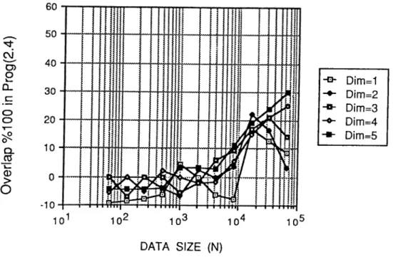
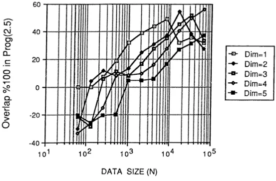
All programs presented in this chapter have been coded in C language and run on an 32-node iPSC/2 hypercube multicomputer for various N = 2" data sizes, 64 < < 64K. Figure 2.6 and Figure 2.7 displays the variation of percent overlap achieved in Prog. 2.4 and Prog. 2.5 respectively. Total communication time and overlapped communication times in Prog. 2.4 and Prog. 2.5 are com­ puted by running Prog. 2.3 without invoking csend and crecv communication routines and subtracting these timings from the original execution timings of Prog. 2.3, Prog. 2.4 and Prog. 2.5 respectively. Percent overlap is then com­ puted by dividing overlapped communication times by total communication times. As is seen in Figure 2.6 and Figure 2.7, percent overlap increases with increasing data size as expected. Note that, for-loop overhead is also included in these timings.

For small data sizes, the amount of computation is not large enough to achieve complete overlap of the communication (Eq. 2.7). Hence, negative per­ cent overlap values are obtained for small data sizes. The oscillations seen in Figure 2.6 and Figure 2.7 for small data sizes are due to the resolution of the system clock used for timings. As is also seen in Figure 2.6 and Figure 2.7, percent overlap begins to decrease slightly after reaching a maximum value at large data sizes (16/i" < N f 2 P < Z2K).

This decrease is closely related to the change in variation of a for those large data sizes. A maximum overlap of % 23 and % 54 are obtained in Prog. 2.4 and Prog. 2.5 respectively in spite of the for-loop overhead. Also, as is indicated

CHAPTER 2, THE FAST FOURIER TRANSFORM 26 cJ o> o CL· C O 0 1— Q. _cd 1 0) > O - o _Dim=1 Dim=2 -B- Dim=3 -0- _Dim=4 ♦ Dim=5 DATA S IZ E (N)

Figure 2.6. Percent Overlap curve for Program (2.4) compared to Pro­ gram (2.3).

in [6], a complete overlaj) cannot be achieved due to the internal architecture of an individual iPSC/2 processor. Figure 2.8, illustrates the variation of per­ cent performance improvement of Prog. 2.3 compared to Prog. 2.2 during the

d exchange communication phases. As is seen in Figure 2.8, Prog., 2.3 outper­

forms Prog. 2.2 as expected since it achieves jrerfect load balance and reduces volume of communication by a factor of two compared to Prog. 2.2. As is also seen in Figure 2.8, percent performance improvement of Prog. 2.3 compared to Prog. 2.2 increases with increasing data size.

Figure 2.9 and Figure 2.10 disjilays the variation of percent jjerformance improvement of Prog. 2.4 and Prog. 2.5 compared to Prog. 2.3 during the d exchange communication phase. As is seen in Figure 2.9 and Figure 2.10, the variation of percent performance improvement is very similar to the variation of overlap curves in Figure 2.6 and Figure 2.7 as expected. As is seen in Fig­ ure 2.9, Prog. 2.4 gives better performance results compared to Prog. 2.3 for

N / P > 8K (e.g. N=16K and P = 2). On the other hand, as is seen in Fig­

LO O) o 1L_ ü_ O O Q. _(0 \_ Q) > o 10'^ 10 DA TA S IZ E (N) -D- _Dim=1 Dim =2 Hl· _{Dim =3} -0- _{Dim =4} Dim =5

Figure 2.7. Percent Overlap curve for Program (2.5) compared to Pro­ gram (2.3).

N / P > 32 (e.g. N=256 and P=4). Comparing Prog. 2.4 and Prog. 2.5, obvi­

ously Prog. 2.5 outperforms Prog. 2.4 for all N. Ttiis result is expected since the introduced overheads both in Prog. 2.4 & Prog. 2.5 are equal compared to Prog. 2.3. Furthermore in Prog. 2.4 only sei}d operation is overlapped while in Prog. 2.5 both send and receive operations are overlapped.

The main reason wdiy Prog. 2.4 and Prog. 2.5 doesn’t give better perfor­ mance results compared to Prog. 2.3 for N / P < 8K and N / P < 32 is due to the extra overhead which is introduced with the second for-loop. This for-

loop overhead in the algorithm cannot be assumed to be negligible and must be

taken into account since it is equal to Upsec/FFT point (experimentally calcu­ lated value). While on the other hand an empty for-loop overhead is equal to

1.2fisec/FFT point. The reason whj' this for-loop introduces a considerable

amount of overhead (i.e., more than an empty for-loop is heavily dependent on the structure of 80387 and the compiler used in the iPSC/2 system.

CHA PTER 2. THE FA ST FO URIER TRA NSFORM 28 CO O) o qI c o o c CD E 0) > 2 Q . E -D- Dim=1 Dim=2 -n- Dim=3 -0- _Dim=4 Dim=5

Figure 2.8. Percent Improvement of Program (2 the last d-stages.

over Program (2.2) during

O) o CL C o o c 0 E 0 > o I— CL E HQ- Dim=1 Dim=2 -D- _Dim=3 -O- Dim=4 Dim=5

Figure 2.9. Percent Improvement of Program (2.4) over Program (2..3) during the last d-stages.

UO O) o CL C o o c CD E 0 > o Q-E -Q. _Dim=1 Dim=2 Dim=3 -0- Dim=4 Dim=5

Figure 2.10. Percent Improvement of Program (2.5) over Program (2.3) during the last d-stages.

ir> o> 0 1— CL C CL Z )₁ Q LU Lll Q. (f) 4 8 12 16 2 0 2 4 2 8 3 2 Number Of Processors -D- LINEAR N =64 -0- _{N =256} -0- _N=1K N=4K N=16K N=64K

CHAPTER 2. THE FAST FOURIER TRANSFORhi 30 -D- _Dim=1 Dim=2 -D- _Dim=3 -O- _Dim=4 Dim=5

Figure 2.12. Efficiency curve for Program (2.5).

As is seen in Figure 2.11, almost linear speed-up is acieved for N > IK. As is seen, in Figure 2.12, efficiency remains over %90 when N / P > 256 F F T points mapped to an individual processor of the hypercube.

2.5

C onclusion

In this chapter we have discussed three efficient parallel F F T algorithms for coarse-grain, distributed-memory, message-passing multiprocessors implement­ ing the hypercube interconnection topology. The first proposed parallel FFT algorithm, Prog. 2.3 achieves both perfect load balance, reduces the volume of communication by a factor of two and doesn’t introduce any memory over­ head. The second proposed parallel F F T algorithm, Prog. 2.4 overlaps one fifth of the computation with only the send portion of communication using

asynchronous send and stjnchronous receive. This method introduces an ex­

tra. send buffer of length N ¡2P. The third proposed parallel F F T algorithm. Prog. 2.5 overlaps one fifth of the computation with both send and receive por­ tions of communication using asynchronous scnd/rcceive. This method further introduces an extra receive buffer of length N / P .

The overall improvement in Prog. 2.4 L· Prog. 2.5 according to Prog. 2.3 is rather small in our case (i.e., for a maximum cube dimension of 3). The reason is, d concurrent exchange phase of the F F T algorithm takes very small amount of time in the overall computation. Also a complete overlap cannot be achieved due to the internal architecture of an individual iPSC/2 processor [6]. Obviously algorithms perform better on higher cube dimensions. Also for different architectures which can achieve complete overlap, the performance index of Prog. 2.4 and Prog. 2.5 will be much higher.

3. T he Fast H artley Transform

3.1

In trod u ction

The Fourier transform allows signals to be treated in the complex frequency domain. If the signals in the time domain are real, then the Fourier transform contains redundancy. The Fast Hartley Transform is an alternative compu­ tation to the complex Fast Fourier Transform when the input signal to be transformed consists of real numbers only. The Fast Hartley Transform is as fast as or faster than the Fast Fourier Transform and still serves for all needs in the digital signal processing world where Fourier transform is presently applied.

Recalling the Discrete Fourier Transform for an input sequence /( ) is,

N - l

F{k) = ^(/(¿)[C'os(27rA:i7A^) -i.9m(27riti7iV)]) (3.1)

t = 0

where (k = 0 ,l,..., N-l) and N is the length of input sequence. As one can see. Discrete Fourier Transform as well as its fast transform includes complex arithmetics. For a more efEcient, simple and faster transformation, the Hartley transform was developed [11]. Its discrete form is ,

N - l

H{k) = ^ {h{i)[Cos(2wki / N) + Sin(2Trki/N)]) (3.2)

i=0

where the input sequence h{) is constrained to real numbers only.

Hartley transform does not neccesitate any complex arithmetics. This im­ portant feature of the Hartley transform increases the performance of D H T by

a factor of two, while decreasing the memory requirements again by a factor of two at the same time. Both of the discrete transformations have a computation time which is proportional to N'^. Fast Fourier Transform reduces this time to A^log2 N [1]. Similar methods can also be applied to the Hartley transform and one can easily obtain a fast transformation for Hartley called Fast Hartley Transform or shortly F H T [12, 13]. There are several Fast Hartley Transform algorithms named as Radix-2 Decimation-in-Time F H T , Radix-2 Decimation- in-Frequency F H T , Radix-4 F H T , Split Radix F H T , Recursive F H T and Vector F H T [14, 15, 16, 17]. One can also calculate F H T through F F T or vice versa [14].

The Fast Hartley Transform presented in Section 3.2 is a decimation-in- time, radix-2 algorithm as presented in [15]. In Section 3.3, static mapping and parallelization of the choosen F H T scheme is discussed. Section 3.3.1 presents the proposed restructuring of the F H T algorithm for an efficient par­ allelization. The dynamic mapping scheme proposed for the restructured F H T algorithm is also presented in Section 3.3.1. Section 3.4 presents the experimen­ tal results and performance evaluation of the proposed algorithms on Intel’s iPSC/2 hypercube multicomputer.

3.2

S eq u en tia l F H T A lg o rith m

Computational steps for a 32-point radix-2, decimation-in-time F H T algo­ rithm is illustrated in Fig. 3.1. This tabular representation is proposed in [17]. The input in this scheme is A^-real numbers in bit-reversed order. The out­ put is iV-real numbers in normal order. The C{i) and S{i) factors Fig. 3.1 represent Co${2'KilN) and Sm{27rilN) respectively. As is seen in Fig. 3.1, each level of F H T algorithm takes a set of N real numbers and transforms them into another set of N real numbers. This process is repeated n = logj N times, resulting in the in-place computation of the desired Discrete Hartley

T r a n s f o r m in normal order. However the tabular representation is not suf­

ficient for a detailed analysis of the computational interdependencies which is crucial for an efficient parallel algorithm design. In this work, computational