A n Intelligent Backtracking S c h e m a
in A Logic P r o g r a m m i n g E n v i r o n m e n t
I l y a s C i c e k l i
Dept. of Comp. Eng. and Info. Sc., Bilkent University 06533 Bilkent, Ankara, Turkey, e-mail: [email protected]
A b s t r a c t
We present a new method to represent variable bindings in the Warren Abstract Machine (WAM), so that the ages of variable bindings can be easily found using this new representation in our intelligent backtracking schema. The age of a variable bound to a non-variable term is the youngest choice point such that backtracking to that choice point can make that variable an unbound variable again. The procedure backtracking point is the choice point of the procedure currently being executed or the choice point of its first ancestor having a choice point. Variable ages and procedure backtracking points are used in the process of figuring out backtracking points in our intelligent backtracking schema. Our intelligent backtracking schema performs much better than the results of other intelligent backtracking methods in the literature for deterministic programs, and its performance for non-deterministic programs are comparable with their results. K e y w o r d s : Logic Programming, Intelligent Backtracking, Prolog, Abstract Machine.
1
I n t r o d u c t i o n
T h e backtracking method used in a standard Prolog implementation is known as naive backtracking. In naive backtracking when a goal fails, backtracking is done to the most recent choice point during that failure (last alternative), although this choice point m a y be nothing to do with that failure. In this approach, a lot of unnecessary backtrackings will be done even though the same failure occurs many times. An intelligent backtracking m e t h o d analyzes the reasons of failures to choose proper choice points to avoid redundant backtrackings. The chosen choice point may not be the most recent choice point during that failure. In other words, the alternatives of choice points between the most recent one and the chosen one are discarded without retrying them. If they are retried, the system will reencounter with that same failure.
The Warren Abstract Machine (WAM) is an abstract machine for Prolog execution which consists an instruction set and several data areas on which instructions operate. The WAM is recognized as a breakthrough in the design of Prolog systems and other computational logic systems by the logic programming community. Many commercial [2, 15] and non-commercial [3] Prolog systems based on the WAM are implemented during the last decade. In this paper, we will assume that the reader is familiar with the WAM. The details of the WAM can be found in Warren's original paper [17] and Kaci's tutorial book on the WAM [1].
Many intelligent backtracking schemes [4, 5, 6, 7, 9, 11, 12, 13, 14, 16, 19] are presented to avoid unnecessary backtracking steps. Early works in intelligent backtracking [4, 9, 14] are implemented as Prolog interpreters. Implementations of later works [6, 7, 11, 12] are WAM based systems.
Our intelligent backtracking schema whose some parts are presented in this paper is implemented as an extension of the WAM, like the systems in [6, 11]. Our mechanism is similar to the mechanisms used in those systems except in the way how we keep unification information for variable bindings and how we find reasons of failures. The mechanism to find the ages of variables causing failures is the central part of any intelligent backtracking schema. In this paper we concentrate on a new representation for variable bindings in the WAM, so that the ages of variables can easily be found. The mechanism we propose is naturally integrated into the WAM architecture, and our performance results are better than the performance results of other systems in [4, 6, 11].
The rest of this paper is organized as follows. Section 2 summarizes the related research about intelligent backtracking. Section 3 introduces procedure backtracking points which play an important role in the determination of variable ages. In Section 4, we present unification graphs to give a concrete definition for variable ages of Prolog variables. In Section 5, we present a new representation for bindings of WAM variables and an algorithm to find ages of WAM variables bound to non-variable terms. The mechanism used in figuring out the intelligent backtracking point for a proced~ure call failure is described in Section 6. Finally, we present some of the performance results in Section 7.
2
R e l a t e d Research
T h e research on intelligent backtracking started in the late 70's. The initial proposals were made by Bruynooghe and Pereira [4], and Cox and Pitrzykowski [9]. These two systems are implemented by extending Prolog interpreters. These methods collect information about bindings during unification and analyze it to determine the intelligent backtracking point when failure occurs. They also retain information from a failure to ensure that a failure is not repeated for the same reason. These methods are known as intelligent backtracking methods based on unification failure analysis. Our backtracking schema has similarities with Bruynogghe's work in the sense that we also collect information about bindings by tagging bindings and
determine the intelligent backtracking points by analyzing these tagged bindings during failure. However our schema is implemented as a WAM-based system, theirs is a Prolog interpreter.
Lin, Kumar and Leung's schema [10, 11, 12] chooses intelligent backtracking points by doing an analysis of literals instead of the analysis of unification failures. In their early work [10], they used the data dependency technique at the clause level for parallel execution of logic programs. A similar mechanism is used by Woo and Choe [19] for A N D / O R parallel process models. Lin and Kumar [11, 12] extend their method for sequential execution of Prolog by using the data dependency technique for the whole proof tree instead of the data dependency technique at the clause level. Later they integrated their technique into the WAM. In their WAM-based implementation they maintain a list of goals for each goal, called B-list, to represent goals such that backtracking to that goal may cure failures of goals in that list. They also tag all variables to represent the data dependency graph. These tags are used to figure out bindings causing the failure of a goal. To reduce the overhead for constructing the d a t a dependency graph, Chang and Despain [5] construct a worst-case data dependency graph at compile time for each clause. Since backtrack literals are chosen at compile time, their schema has a little bit overhead at run time. However, this method is not capable of handling better situations at run time, because it tries to meet the requirements of the worst case. This method also needs information about possible activations of goals before the compile time analysis. This information must be given by the user. Without this information, this static data-dependency analysis may degenerate into the naive backtracking. So, the main responsibility is on the user and the efficiency of this method depends on how well the possible activations of goals are marked.
Codognet and his colleagues propose a depth-first intelligent backtracking schema in [6] and they give its WAM-based implementation in [7]. In their schema, unification instructions record the source of bindings and failure routines choose the intelligent backtracking point and update sets of intelligent backtracking points. During unifications, they create a simplified version of the unification graph which records the time of bindings. They also attach a set of intelligent backtracking points to each literal. These sets are created at first entrances to literals, and they are maintained during the backtracking process. To minimize the maintenance overhead of these sets, bit-vectors are used to implement them. They claim that the forward overhead of their schema which occurs during unifications is 1 0 - 15% compared with the WAM, and the backward overhead which occurs during failures is 5%. They accept that the total overhead for deterministic programs is 20%.
Toh and Ramamohanrao [16] propose an intelligent backtracking schema that does not require a data-dependency analysis or information to be collected during unification. According to their method, the failed atom is itself used to figure out the intelligent backtracking point. Since a failure-directed mechanism is less accurate than a unification-based schema, their schema gives less accurate results compared to other unification based schemes including our schema.
Most of the intelligent backtracking methods in the literature associate some kind of sets with literals to store intelligent backtracking points. These sets are called alternative backtracking points in [6, 7], B-lists in [12], rejected procedures in [4], witness sets in [18] and candidate sets in [8]. These sets have to be updated either during unification or during failure. The main difference of our method is that we do not have to maintain this kind of sets. In our method, we tag bindings during unifications and use the information in tagged bindings to figure out intelligent backtracking points during failures. The most of the overhead in our method occurs when we try to find the intelligent backtracking point during a failure. In other methods, the big percentage of the overhead of the intelligent backtracking mechanism occurs when they maintain these sets. Since some of these methods create these sets during the unification, they pay a heavy penalty even in deterministic programs. In our mechanism, however, we pay the penalty during failures, and therefore our gain from the intelligent backtracking mechanism in nondeterministic programs can compensate these overheads. Since our mechanism has a little overhead during unification, these overheads do not cause big penalties in deterministic programs. In fact, the forward overhead of our schema which occurs during unifications is only 2 - 3%.
3
P r o c e d u r e Backtracking P o i n t s
In a regular Prolog system, a backtracking is made to the most recent choice point when a failure occurs due to a unification. This failure occurs because a variable bound to a non-variable term cannot be unified with a different non-variable term or the unification algorithm cannot unify two variables bound to two different non-variable terms. Since a variable bound to a non-variable term is responsible of that failure, the reoccurrence of that failure can only be avoided by backtracking to a choice point such that this variable will not be bound to that non-variable term when that same unification occurs. So, a backtracking to the most recent alternative in a regular Prolog system may not fix the problem and that same failure may occur again. Thus, we should backtrack to the youngest choice point such that the variable causing the failure can be unbound again. This choice point will be called as the reason of that failure. We can also avoid that failure by backtracking to the first alternative of the clause in which that failure occurs. This means that we wilt completely skip the clause where the unification causing that failure occurs. Of course, the youngest one of these two points is going to be the backtracking point for that failure in our intelligent backtracking schema. Now, we give a definition to formaUy describe the procedure backtracking point.
D e f i n i t i o n 3.1 ( P r o c e d u r e B a c k t r a c k i n g P o i n t ) Let p be the current procedure being executed. The procedure back- tracking poinl at a certain lime of execution is:
* the choice point of p if p has a chowe point
. the choice point of p's first ancestor which has a choice point ofherwise
r p q p
g - - - X Y ... Z X f(Y)
Notation: ]
Variables X and Y were unified when the choice point q
X P Y of procedure p was the procedure backtracking point, g
a. A Unification G r a p h with Variables b. A Unification Graph with Terms
Figure 1: Unification Graphs
T h e procedure backtracking point indicates the furthest choice point to which the system can backtrack during a failure. When a failure occurs, the system should backtrack to a choice point between the m o s t recent one and the procedure backtracking point. If the procedure backtracking point is equal to the most recent choice point, this is known as shallow backtracking. In t h a t case, the most recent choice point is tried. If the procedure backtracking point is older than the m o s t recent choice point, in t h a t case the point t h a t the system will backtrack depends on the reason of the failure. If the reason of t h a t failure indicates a choice point which is older than the procedure backtracking point, we can only backtrack up to the procedure backtracking point. By backtracking to the current procedure backtracking point, we completely skip the clause where the unification causing that failure occurs. In other words, we will not reencounter with that same failure because we are not going to execute that unification again.
In the WAM based implementation of our intelligent backtracking schema we introduce a new register PB (Procedure Backtracking Point) to hold the procedure backtracking point in addition to the registers in the original WAM architecture. T h e register PB is u p d a t e d with a new choice point which is created by a try instruction. The previous value of the register PB is saved in the new choice point by t h a t try instruction. During a backtracking, this register is changed to point to the backtracked choice point. In fact, that choice point is the most recent choice point at t h a t time. T h e register PB is also restored with the saved value in a choice point when t h a t choice point is discarded.
T h e PB register is saved in the environments by the allocate instruction in the s a m e way as saving the environment register E, except that the register PB is not u p d a t e d by the allocate instruction. The reason of saving it in environments is that it can be restored with the stored value in the current environment by the proceed instruction. When a proceed instruction is executed, we get out from a context of a procedure and return to the context of one of its ancestors. Since t h a t ancestor has an environment and its procedure backtracking point is saved in its environment, the register PB can be restored with t h a t value.
4
Unification Graphs
In this section, we introduce unification graphs to represent the unifications of variables in a Prolog program. T h e aim of this section is to define the concept of the age of a eariable in a Prolog environment. T h e age of a Prolog variable (bound to a non-variable term) which causes a failure plays an i m p o r t a n t role to figure out the intelligent backtracking point for t h a t failure.
A unification graph for a set of variables is a labeled acyclie undirected graph such that vertices of t h a t graph are variables in that set and an edge represents the unification of variables indicated by two vertices. T h e label on an edge indicates the age of t h a t unification.
The age of a unification is the procedure backtracking point during t h a t unification. T h e backtracking to the choice point indicated by the age of a unification can avoid the reoccurrence of that unification. In other words, the backtracking to the age of a unification will completely skip the clause where that unification occurs.
Figure 1.a gives a unification graph for three variables X, Y, Z and a non-variable term g. Labels on edges are the names of procedures whose choice points are the procedure backtracking points during those unifications. In the example, X is unified with Y and g such that the procedure backtracking points during these unifications are the choice points of procedures p and r, respectively. During the unification of Y and Z, the choice point of procedure q is the procedure backtracking point. Note that, all variables are bound to non-variable term g as the result of three unifications in that graph. T h e labels on edges do not reflect the times of unifications. T h a t is the three unifications given in the graph of Figure 1.a can be performed in any order.
The age of a Prolog variable which is bound to a non-variable term is the youngest one among the choice points indicated by the labels on the path from t h a t variable to t h a t non-variable term in a unification graph. If a failure occurs because of a variable which is bound to a non-variable term, the backtracking to any one of the choice points indicated by the labels on the p a t h from that variable to that non-variable will avoid the reoccurrence of that failure. In Figure 1.a, Z is bound to
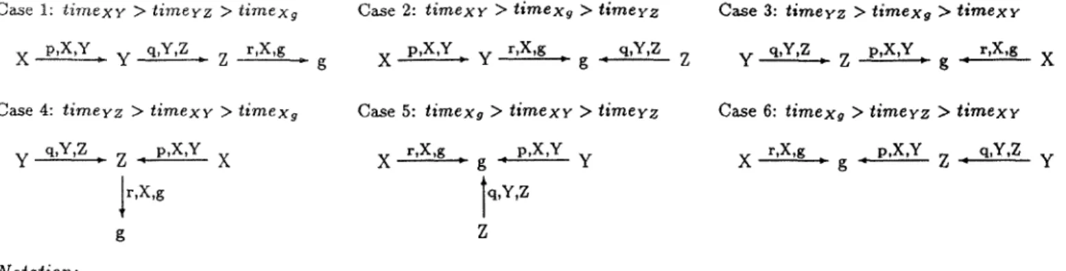
Case 1: t i m e x y > t i m e y z > t i m e x 9 X p,X,Y y q , Y , Z Z r,X,g Case 2: t i m e x Y > t i m e x g > t i m e y z X p,X,Y , . y r,X,g P g ' q,Y,Z Case 3: t i m e y z > t i m e x a > t i m e x r Z y q,Y,Z , Z p,X,Y,, g ~ r,X,g X Case 4: t i m e y z > t i m e x y > t i m e x g y q,Y,Z , Z - p,X,Y X
l
r,X,g g Notation: L1 p , X , Y L2 t i m e x y : Assumption :Case 5: timexg > t i m e x v > t i m e r z Case 6: timexg > timeyz > t i m e x r
X r,X,g g p,X,Y Y X r,X,g p,X,Y q,Y,Z
" " ' g ° Z " Y
'[q,Y,Z
Z
Location LI is bound to location L$ because o] a unification such that the age o] that unification is p and variables involved in that unification are X and Y.
Time of the unification of X to Y. Relations < and > will be used to indicate younger and older relations among times. Creation order .for variables is g, if, Y, and X and all o] them live on the same data area (the heap).
Figure 2: Corresponding Reference Chains For A Unification Graph
t e r m f(Y) to figure out the intelligent backtracking point. In the second case, we use the youngest one of the unification ages on paths from X to f(Y) and from Y to g.
5
A g e s of W A M Variables
In this section, we present a new representation technique for bindings of WAM locations, and discuss variable ages in terms of binding ages of WAM locations. We do not use unification graphs directly in our WAM based implementation. A unification graph can be m a p p e d into different structures of WAM locations. We can calculate the age of a WAM location corresponding to a Prolog variable in each of these different structures of WAM locations.
A variable in the WAM is a chain of locations ending with an unbound location or a non-variable term. Since non- variable terms cause failures during unifications, we will concentrate on reference chains ending with non-variable terms. If an unbound location is bound to another location, this operation is called binding. If a variable having a binding in its reference chain causes a failure because of that binding, we have to backtrack to the procedure backtracking point at the time of t h a t binding. Note that the age of a binding m a y not be the most recent choice point at the time of t h a t binding. In the following example, the ages of the bindings similar to the bindings of variables X and Y must be equal.
p :- X = l , q, Y=2, s(X,Y), q. Ages of bindings of X to 1 and Y to 2 are equal, namely the choice point of p. p. q. Note that the most recent choice points are different during these bindings. T h e age of both of those bindings is the choice point of procedure p which is the procedure backtracking point during both of those bindings. Thus, if procedure s fails due to binding of Y to 2, we should backtrack to the choice point of p instead of the choice point of q.
D e f i n i t i o n 5.1 ( A g e o f B i n d i n g ) The age of a binding is the procedure backtracking point in the register P B at the time of that binding.
This definition corresponds to the definition of the age of a unification in unification graphs. It is obvious t h a t the age of a binding must be equal to the age of the unification causing t h a t binding in Prolog.
Since we need the ages of all bindings, we use extra entries to store information about bindings in our representation. In our method, we use four value cells for each bound WAM location. The first value cell holds the actual value which is stored there as a result of the binding operation. It will be a pointer to another WAM location or a constant. The procedure backtracking point during that binding is saved in the second position. This is the age of the binding and it m a y be different than the most recent choice point during that binding. The third and fourth positions hold the first locations of variables whose unification causes this binding.
A unification graph can be mapped into different structures of WAM locations depending on the times of unifications and creation times of locations for variables in t h a t graph. Let us assume that the locations for X, Y, Z and g in Figure 1.a are created in reverse order (i.e. the creation order is g, Z, Y and X) in the same d a t a area. We can have six different structures for the reference chains of variables depending on the times of three unifications in that graph. Figure 2 gives the reference chains for these six cases. In the figure, an arrow represents a binding, and a label on each arrow represents the age of that binding and the first locations of variables whose unification causes that binding. For example, in Case 5 the
f u n c t i o n age(V:location) : age; {
g ~ location of the non-variable term at the end of the reference chain of V; i f g = V t h e n agev ~ age 9
e l s e { notvisited ~ junctionsetv g; visited ~ empty;
done ~ f a l s e ;
w h i l e ( n o t done ) d o {
delete first node ( ( x, y), ageset~y ) from notvisited;
i f (x,y) = (V,g) t h e n { agesety9 ~ ageset~y; done ~-- t r u e ; } else { f o r e a c h ((w, z), agesetwz) in junctionset~y d o
i f (w, z) -~ (z, y) a n d (w, z) f~ visited a n d (w, z) ~ notvisited t h e n add ((w, z), agesetwz) to notvisited as last node;
f o r e a c h ((w, z), agesetwz) in visited d o
i f (x, y) and (w, z) share a common location t h e n {
let (b, c) be new pair where b, c are other locations in (z, y) and (w, z); if (b, c) ¢ (z, y) a n d (b, c) fE visited a n d (b, c) f~ notvisited t h e n
add ( (b, c), agesetx~ t.J agesetwz ) to notvisited as last node; } add ((z, y), agesetxy) to visited as last node; } }
agey ~ youngest in agesetvg; } r e t u r n agey }
Figure 3: Algorithm to Find Age of Variable Bound To Ground Term
arrow from Z to g with labels q, Y, Z represents the binding of Z to g. The age of that binding is q and the first locations of variables causing that binding are Y and Z. Note that q is also the age of unification of Y with Z in the corresponding unification graph in Figure 1.a.
D e f i n i t i o n 5.2 ( A g e S e t o f B i n d i n g o f T w o L o c a t i o n s ) Let X and Y be two WAM locations and their reference chains join at some location. The age set of binding of X and Y is the set of ages of bindings causing that junction. We will use
the notation a g e s e t z y to represent the age set of the binding of X and Y.
D e f i n i t i o n 5.3 ( A g e o f W A M L o c a t i o n ) Assume that X is a WAM location whose reference chain ends with location G holding a non-variable term. The age of X is the youngest age in agesetxa. We will use the notation agex to represent the age of X.
If the reference chains of two locations end in the same location, they must have a junction location. At the worst case, this junction location is the last location in their reference chains. For example, X and Y in Case 3 of Figure 2 has the location of g as a junction location, but the junction location for Y and Z is Z.
D e f i n i t i o n 5.4 ( J u n c t i o n S e t ) If X and Y have a junction location Z, their junction set is the set of all bindings from X to Z and from Y to Z. We will use the notation j u n c t i o n s e t x y for the junction set of X and Y.
Each item in a junction set is a pair representing a binding. The first element in that pair is also a pair of the first locations of variables whose unification causes that binding. The second element in the binding pair is a singleton set of the age of that binding. For example, the junction set of X and Y in Case 3 of Figure 2 is equal to {((Y, Z), {q}), ((X, Y), {p}), ((X, g), {r})}, but the junction set of Y and Z is {((Y, Z), {q})}. In fact, a junction set is a special form of sets of bindings with age sets. A set of bindings with age sets is the same as a junction set except that the second element in a binding pair can be any non-empty set of ages. A binding age pair ((Y, Z), {q}) means that Y and Z are bound to each other because of a unification whose age is q. In general, the age set in a binding age pair represents the ages of unifications causing the binding of two locations in that pair.
Figure 3 gives an algorithm written in pseudo-code to find tile ages of variables bound to non-variable terms. In that algorithm, we first find the location g of a non-variable term at the end of a reference chain of a given variable V. If V is equal to g, then the age of the location of the non-variable term is the age of V. Otherwise, we have to construct agesetvg which is the set of ages of unifications causing the binding of V to g to find the age of V. We start from the junction set junctionsetvg of V and g to accomplish this task because the age of at least one of the bindings in junctionsetvg will be in agesetvg. We continue to enlarge our set of bindings with age sets by adding junction sets of variables of bindings currently in our set and new bindings are constructed by joining two bindings in our set. Two bindings can be joined to get a new binding if they share a common variable. In other words, if there are bindings (x,y) and (y, z), we create a new binding (x, z). The age set of this new binding will be the union of the age sets of those bindings involved in that join operation. Bindings which have been considered are put into the set visited and the rest of bindings stay in the set
notvisited. New bindings are added to notvisited if they have not been produced earlier. During the enlargement of the set, we check whether we find the binding of V and g, or not. The enlargement stops when we find it. This algorithm is a breath first search in the search space of all possible bindings. Since the age of a variable is the youngest age in its age set, we compute the youngest age in its age set instead of computing the whole set in the actual implementation of this algorithm.
Example :
This example shows the enlargement steps while the algorithm tries to find the age of Z in Case 3 of Figure 2. At each step, we give the sets visited and notvisited to indicate the current search space of bindings.
, Calculate junctionsetzg and assign it to notvisited. notvisited = {((X, Y), {p})} visited = {}
• Visit (X, Y ) by adding junctionsetxy and the results of join operations of ((X, Y), {p}) with all bindings in visited to notvisited.
notvisited = {((Y, Z), {q}), ((X, g), {r})} visited = {((X, Y), {p})} • Visit (Y, Z) by adding junetionsetyz and the results of join operations of
((Y, Z), {q}) with all bindings in visited to notvisited.
notvisited = { ( ( X , g ) , { r } ) , ( ( X , Z ) , { p , q } ) } visited = { ( ( X , Y ) , { p } ) , ( ( Y , Z ) , { q } ) } ® Visit (X, g) by adding junctionsetxg and the results of join operations of
((X, g), {r}) with all bindings in visited to notvisited.
notvisited = {((X,Z),{p,q}),((Y,g),{p,r})} visited= { ( ( X , Y ) , { p } ) , ( ( Y , Z ) , { q } ) , ( ( X , g ) , { r } ) } ® Visit (X, Z) by adding junctionsetxz and the results of join operations of
((X, Z), {p, q}) with all bindings in visited to notvisited.
notvisited = {((Y, g), {p, r}), ((Z, g), {p, q, r})} visited = {((X, Y), {p}), ((Y, Z), {q}), ((X, g), {r}), ((X, Z), {p, q})} • Visit (Y, g) by adding junctionsety 9 and the results of join operations of
((Y, g), {p, r}) with all bindings in visited to notvisited.
notvisited = {((Z, g), {p, q, r})} visited = {((X, Y), {p}), ((Y, Z), {q}), ((X, g), {r}), ((X, Z), {p, q}), ((Y, g), {p, r})} • Visit (Z,g). We found agesetzg.
agesetzg = {p, q, r}
® Choose the youngest age in agesetzg as agez.
To optimize our algorithm, we can stop the search immediately after the binding ((Z, g), {p, q, r}) is found during the visit to the binding ((X, Z), {p, q}).
6
F i n d i n g t h e R e a s o n s o f a P r o c e d u r e F a i l u r e
A failure normally occurs during the unification of head arguments. Unification instructions used in head matching can be divided into two groups. Instructions in the first group (e.g. get_constant and unify_constant ) try to unify a variable with a specific non-variable term. A failure occurs when that variable is bound to a non-variable term which is different than that specific non-variable term. The second group instructions (e.g. get_val and unify_va 0 are complete unification instructions which take two variables to be unified. In this case, a failure occurs when those variables are bound to two different non-variable terms. In the first case, the age of that variable determines the reason of that failure. In the second case, the youngest one of the ages of two variables plays role in the determination of the reason of that failure. In both cases, the reason of the failure will point to the choice point which is actually the procedure backtracking point during the binding causing that failure.
A procedure call fails if all clauses of that procedure fail. T h e reason of the failure of that procedure call is the youngest one of failure reasons of its clauses. To store the youngest reason of a procedure failure, we reserve a space in choice points. After this point, we call that field in choice points as t~B (Reason Backtracking Point). This field is initialized by a special value during the creation of that choice point by try instructions. During a failure, the RB field of the choice point indicated by the procedure backtracking point register PB may be updated with the reason of that failure. It is updated with the reason of that failure, only if that reason is younger than the value stored in RB field. So, RB field always holds the youngest one of failure reasons of the clauses of the procedure in question.
When a failure occurs with a failure reason R which points to a choice point, the failure routine compares R with the value stored in register PB. If R is younger than PB, R is chosen as the backtracking point. This means that we stay in the context of the current clause of the procedure owning the choice point indicated by PB. In other words, that clause has not failed yet. If R is equal to PB, the clause of the procedure owning the choice point indicated by PB fails, but this failure does not depend on any outside reason. In this case, IR is again chosen as the backtracking point. If R is older than PB, the clause fails due to an outside reason. Since the procedure has other alternatives, backtracking point is the next alternative in the choice point indicated by PB register. Since a clause of the procedure in question fails, the reason of that clause failure may be needed to be recorded in RB field of its choice point. Of course, that reason is only recorded if it is younger than the failure reasons of previous clauses of that procedure.
mapcolor(A,B,C,D,E) :-
next(A,n), next(A,C), next(A,D), next(A,E), next(B,C).
next(X,Y) :- nextl(X,Y). next(X,Y) :- nextl(Y,X).
Figure 4: Map Coloring
nextl(green,red). nextl(green,yellow). nextl(green,blue).
next 1 (red,yellow). next 1(red,blue). next 1 (yellow,bl ue).
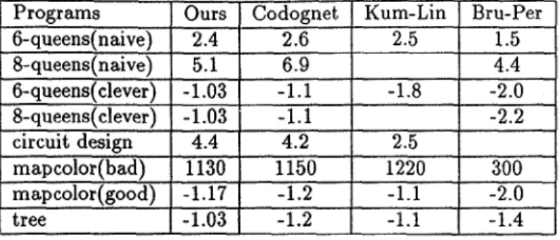
Programs Ours 6-queens(naive) 2.4 8-queens(naive ) 5.1 6-queens(clever) -1.03 8-queens(clever) -1.03 circuit design 4.4 mapcolor(bad) 1130 mapcolor(good) -1.17 tree -1.03
Codognet Kum-Lin Bru-Per
2.6
2.5
1.5
l
6.9 4.4 -1.1 -1.8 -2.0 ] I -1.1 -2.2 4.2 2.5 1150 1220 300 -1.2 -1.1 -2.0 -1.2 -1.1 -1.4Table 1: Speedups of Intelligent Backtracking Methods w.r.t. Prolog
Since we need to choose the youngest reason among the failure reasons of the clauses of a procedure as the failure reason of the procedure call to that procedure, we also need the failure reason of its last clause to make this decision. This means t h a t the choice point of a procedure should not be discarded before its last clause fails. For this reason,
trust
instructions in our implementation do not discard choice points. T h e y behave the same way asretry
instructions except that they put the address of a new WAM instructiondiscardfail
instead of the address of the next clause in choice points. When the last clause of a procedure fails, this new instructiondiscardfail
is executed to discard the most recent choice point and to invoke a failure with the reason stored in RB field of that choice point. This means that the procedure call is going to fail with the youngest one of the failure reasons of its clauses. Note that we do not need to create a choice point for procedures with a single alternative. The failure reason of the procedure call to such a procedure is the failure reason of its single clause.7
P e r f o r m a n c e
R e s u l t s
We have extended the byte emulator of the WAM based system of ALS (Applied Logic Systems) Prolog to implement our mechanism. To observe the gains and the overheads of our system, we tested it with programs in three categories in addition to the standard test programs for intelligent backtracking systems.
The first category includes programs which do a lot of unnecessary backtrackings in a regular Prolog system. Our system gives a good performance in these programs, because it avoids a lot of redundant failures. A map coloring program given in Figure 4 is a good example for this category. In a regular Prolog system, there are 147 failures before it finds a solution. In our system, there are only 15 failures. In terms of cpu time, our system is 6 times faster than the Prolog system for that example. In the program, the last subgoal fails for the first values of variables B and C. In a regular Prolog system, all alternatives of the third and the fourth subgoals are tried before the second subgoal is retried to get another value for variable C although they are not responsible for the binding of variables B and C. In our schema, when the last subgoal is completely failed, the system backtracks to the next alternative of the second subgoal without retrying the third and the fourth subgoals.
The second category contains Prolog programs that do a lot of backtrackings but only a few of them are redundant. This kind of programs use all machinery in our schema without any gain. In fact, this kind of programs represent the worst case for our schema. For example, if we put the subgoal next(B,C) as the third subgoal in the clause in Figure 4, there will not be any redundant failures. In that case, our system and a regular Prolog system do the same backtrackings. The slow-down in our system is 17 percent compared with the regular Prolog system.
Deterministic programs are in the last category. Since most of the overheads in our schema occur during the failure analysis, we want to see its effects on deterministic programs. We tested our system with a completely deterministic program, and the slow-down in our system was only 2-3 percent. This result is a real encouragement because the overhead in our schema is minimum when there are few failures. In fact, this reflects the overhead of keeping extra information for binding operations, maintaining PB register, and storing that register in choice points and environments. If there are a lot of failures, the gains by avoiding redundant backtrackings are more than the overheads due to a more complex failure routine.
We also tested our implementation with certain benchmarks to compare our results to other intelligent backtracking methods presented in [4, 7, 12]. Table 1 shows speed ups and slow downs of the intelligent backtracking methods with respect to different Prolog systems. Our figures in the table give a comparison of our intelligent backtracking scheme to the byte-emulator of ALS Prolog. Positive numbers reflect speed ups in intelligent backtracking schemes, and negative
numbers reflect slow downs. Table 1 shows that speed ups of our scheme are not worse than the results of other methods for nondeterministic programs such as naive versions of N-queens problem, circuit design problem and bad version of map coloring problem. The good version of map coloring problem reflects the worst case of our scheme because there are a lot of failures in that program and we do not gain much from the intelligent backtracking scheme for that problem. This means that our worst case is still as good as other methods. The best part of our scheme is its low overhead on deterministic programs. Slow downs of our scheme for deterministic programs such as clever version of N-queens problem and tree problem are much better than the results of other methods for the same problems.
8
C o n c l u s i o n
Our intelligent backtracking mechanism whose some parts are presented here chooses the youngest choice point for back- tracking during a failure such that backtracking to that choice point can avoid the reoccurrence of that same failure. It is guaranteed that the chosen backtracking point is the youngest choice point such that backtracking to any choice point younger than the chosen choice point cannot avoid the recoccurence of that same failure. This means that our mechanism chooses exactly the right position for backtracking.
The new method for the representation of bindings of WAM variables plays an important role in the process of finding the ages of variables bound to non-variable terms. The age of a variable and the procedure backtracking point introduced here determine the backtracking point during a failure due to that variable. This new representation is smoothly integrated into the original WAM architecture with small overheads. Since most of the overheads of our system occur during a failure (not during a unification process), it is more suitable for an intelligent backtracking schema because the overheads during unification will occur in every type of program.
R e f e r e n c e s
[1] Ait-Kaci, H., Warren's Abstract Machine: A Tutorial Reconstruction, MIT Press, Cambridge, 1991. [2] ALS Prolog Manual, Applied Logic Systems. Inc., 1992.
[3] Bowen, K.A., Buettner, K.A., Cicekli, I., and Turk, A., A Fast Incremental Portable Prolog Compiler, Lecture Notes in Computer Science 225, Springer-Verlag, New York, 1986.
[4] Bruynooghe M. and Pereira L. M., Deduction Revision by Intelligent Backtracking, in Implementations of Prolog, ed. Cambell J. A., Ellis Horwood, 1984.
[5] Chang J.-H. and Despain A. M., Semi-Intelligent Backtracking of Prolog Based on a Static Data Dependency Analysis, Proc. of 2 "d Int. Symp. on Logic Programming, Boston, 1985.
[6] Codognet P., Codognet C. and Fil~ G., Yet Another Intelligent Backtracking Method, Proc. of 5 th Int. Conf. and Syrup. on Logic Programming, Seattle, 1988.
[7] Codognet P. and Sola T., Extending the WAM for Intelligent Backtracking, Proc. of 8 th Int. Conf. on Logic Program- ming, Paris, 1991.
[8] Conery J.S., Implementing Backward Execution in Nondeterminislic AND-parallel Systems, Proc. of 4 th Int. Conf. on Logic Programming, Melbourne, 1987.
[9] Cox P. and Pietrzylowski T., Deduction Plans: A Basis for Intelligent Backtracking, IEEE PAMI, Vol 3, 1981. [10] Lin Y-J., Kumar V. and C. Leung, An Intelligent Backtracking Algorithm for Parallel Execution of Logic Programs,
Proc. of 3 ~a Int. Conf. on Logic Programming, London, 1986.
[11] Lin Y-J. and Kumar V., An Intelligent Backtracking Schema for Prolog, Proc. of 4 th Int. Syrup. on Logic Programming, San Francisco, 1987.
[12] Lin Y-J. and Kumar V., A Data-Dependency Based Intelligent Backtracking Schema for Prolog, J. Logic Programming, Vol 4, 1988.
[13] Matwin S. and Pietrzylowski T., Intelligent Backtracking in Plan Based Deduction, IEEE PAMI, Vol 7, 1985.
[14] Pereira L. M. and Porto A., Selective Backtracking, in Logic Programming, ed. Clark K. L. and Tarnlund S.-A., Academic Press, 1982.
[15] Quintus Prolog Reference Manual, Quintus Computer Systems Ltd., 1991.
[16] Toh J. and Ramamohanrao K., Failure Directed Backtracking, Tech. Report 86/9. CS Dept., Univ. of Melbourne, Australia, 1986.
[17] Warren D.H.D., An Abstract Prolog Instruction Set, SRI Technical Report 309. 1983.
[18] Winsborough W., Semantically Transparent Selective Reset for AND Parallel Interpreters Based on the Origin of Failures, Proc. of 4 th Int. Symp. on Logic Programming, San Francisco, 1987.
[19] Woo N. and Choe K., Selecting The Backtrack Literal in The AND~OR Process Model, Proc. of 3 rd Int. Syrup. on Logic Programming, Salt Lake City, 1986.