ASSESSMENT AND CORRECTION OF ERRORS
IN DNA SEQUENCING TECHNOLOGIES
a thesis submitted to
the graduate school of engineering and science
of bilkent university
in partial fulfillment of the requirements for
the degree of
master of science
in
computer engineering
By
Can Fırtına
December 2017
Assessment and correction of errors in DNA sequencing technologies By Can Fırtına
December 2017
We certify that we have read this thesis and that in our opinion it is fully adequate, in scope and in quality, as a thesis for the degree of Master of Science.
Can Alkan(Advisor)
A. Erc¨ument C¸ i¸cek
Tolga Can
Approved for the Graduate School of Engineering and Science:
Ezhan Kara¸san
ABSTRACT
ASSESSMENT AND CORRECTION OF ERRORS IN DNA
SEQUENCING TECHNOLOGIES
Can Fırtına
M.S. in Computer Engineering Advisor: Can Alkan
December 2017
Next Generation Sequencing technologies differ by several parameters where the choice to use whether short or long read sequencing platforms often leads to trade-offs between accuracy and read length. In this thesis, I first demonstrate the problems in reproducibility in anal-yses using short reads. Our comprehensive analysis on the reproducibility of computational characterization of genomic variants using high throughput sequencing data shows that re-peats might be prone to ambiguous mapping. Short reads are more vulnerable to rere-peats and, thus, may cause reproducibility problems. Next, I introduce a novel algorithm Her-cules, the first machine learning-based long read error correction algorithm. Several studies require long and accurate reads including de novo assembly, fusion and structural variation detection. In such cases researchers often combine both technologies and the more erroneous long reads are corrected using the short reads. Current approaches rely on various graph based alignment techniques and do not take the error profile of the underlying technology into account. Memory- and time- efficient machine learning algorithms that address these shortcomings have the potential to achieve better and more accurate integration of these two technologies. Our algorithm models every long read as a profile Hidden Markov Model with respect to the underlying platform’s error profile. The algorithm learns a posterior transi-tion/emission probability distribution for each long read and uses this to correct errors in these reads. Using datasets from two DNA-seq BAC clones (CH17-157L1 and CH17-227A2), and human brain cerebellum polyA RNA-seq, we show that Hercules-corrected reads have the highest mapping rate among all competing algorithms and highest accuracy when most of the basepairs of a long read are covered with short reads.
¨
OZET
DNA D˙IZ˙IL˙IM TEKNOLOJ˙ILER˙INDEK˙I HATALAR ¨
UZER˙INE
DE ˘
GERLEND˙IRME VE HATALARIN D ¨
UZELT˙ILMES˙I
Can Fırtına
Bilgisayar M¨uhendisli˘gi, Y¨uksek Lisans Tez Danı¸smanı: Can Alkan
Aralık 2017
Yeni Nesil Dizileme teknolojileri bir¸cok de˘gi¸skende birbirleri arasında farklılık g¨ostermektedir. Kısa par¸calı dizileme ya da uzun par¸calı dizileme teknolojileri arasında yapılacak bir se¸cim ise par¸caların do˘gruluk oranı ya da uzunlukları arasında bir tercih gerektirir. Bu tezde ilk olarak, kısa par¸caların kullamıyla yapılan analizlerin yeniden ¨uretilebilirli˘gi konusundaki problemleri belirtiyorum. Yeni nesil dizileme teknolojileri kullanılarak genomik farklılıkların karakter-istikleri ¨uzerinde yaptı˘gımız geni¸s ¸calı¸sma g¨ostermektedir ki tekrarlayan dizileme par¸caları, dizilerin mu˘glak bir ¸sekilde haritalanmasına sebep olabilir. Kısa par¸calar tekrarlamaya daha yatkın olduklarından dolayı bu par¸caların kullanıldı˘gı deneylerin yeniden ¨uretilebilmesinde problemler ya¸sanması m¨umk¨und¨ur. Bu tezde ikinci olarak, ¨ozg¨un bir algoritma olan Her-cules’i sunuyorum. Hercules, uzun par¸calardaki hataların d¨uzeltilmesi i¸cin makine ¨o˘grenimi tekni˘gini kullanan ilk algoritmadır. De novo y¨ontemiyle haritalama, yapısal farklılıkların ara¸stırılması gibi bir¸cok ara¸stırma uzun ve hatasız par¸caların kullanımını gerektirmekte-dir. Bu durumlarda, ara¸stırmacılar genellikle uzun par¸calardaki hataların d¨uzeltilmesini kısa par¸calar ile yapmaktadırlar. C¸ izge yapısı ve hizalama temelli g¨uncel d¨uzeltme y¨ontemleri, dizileme teknolojisinin hata profilini g¨oz ardı etmektedirler. Hata profilini el alan, hafıza ve zaman konusunda elveri¸sli makine ¨o˘grenimi teknikleri, hataları daha iyi d¨uzeltme ve daha her iki teknolojiyi daha iyi birle¸stirme konusunda potansiyele sahiptirler. Sundu˘gumuz algoritma, her bir uzun par¸cayı, kullanılan teknolojinin hata profiline uygun bir profile Hid-den Markov Model’i ¸seklinde tasarlamaktadır. Algoritmamız, ge¸ci¸s ve emisyon olasılıklarını b¨ut¨un uzun par¸calar i¸cin ¨o˘grenip, de˘gi¸stirerek uzun par¸calardaki hataların d¨uzeltilmesini sa˘glamaktadır. DNA diziliminden iki adet veri dizisi (CH17-157L1 ve CH17-227A2) ve RNA diziliminden bir adet veri dizisi (human brain cerebellum polyA) kullanarak, Her-cules tarafından hataların giderildi˘gi par¸caların, di˘ger algoritmalar kullanılarak hataların d¨uzeltilmesine kıyasla en y¨uksek haritalama oranına ve uzun par¸caların b¨uy¨uk b¨ol¨um¨u kısa par¸calarla kaplandı˘gı durumlarda en y¨uksek hatasızlık oranına sahip oldu˘gunu g¨osteriyoruz. Anahtar s¨ozc¨ukler : DNA, dizileme, tekrarlar, hata d¨uzeltme, b¨uy¨uk par¸ca, makine ¨o˘grenimi.
Acknowledgement
I would like to express my sincerest gratitude to my supervisor, Asst. Prof. Can Alkan, who has guided and supported me continuously for three years during both my undergraduate and graduate study at Bilkent University. Without his wisdom, patience, and his support, the studies presented in this thesis would have never been completed. I owe him much more than a gratitude for simply being more than just a supervisor: also a friend, and a role-model. I also would like to thank Asst. Prof. A. Ercument Cicek for suggesting a novel approach for correcting the errors in long reads with the use of profile Hidden Markov Models. His ideas and encouragement led us to introduce a novel method that will hopefully have a good impact on the computational biology field. I also would like to thank him for sharing joyful and insightful conversations with me.
I am also grateful to Asst. Prof. Oznur Tastan for her long-standing support, for being a great supervisor of our senior project, for providing me with the opportunity to be a co-author with her, for her invaluable comments during the preparation of my first published article. I will always consider myself lucky to have my first research experience under her supervision.
I am thankful to Prof. Levent Onural for allocating the generous computational resources for the research we have conducted together. It was a real privilege to conduct a research under his supervision. His wisdom and his guidance have already shaped the path that I took for my research career.
I thank Prof. Tolga Can for giving his precious time to read this thesis.
I acknowledge T ¨UB˙ITAK-1001-215E172 grant and a Marie Curie Career Integration Grant (303772).
The last but not the least, I would like to thank my mother and father, Emine and Turan Fırtına, for their endless love, dedication, and their support. I will always be grateful to them for believing in me. I would like to dedicate this thesis to my mother and my father so I can carry a piece from them even when we live far away.
Contents
1 Introduction 1
2 Effects of read length and genomic repeats on the reproducibility of
ge-nomic analyses 6
2.1 Methods . . . 6
2.1.1 Data acquisition . . . 6
2.1.2 Read mapping, shuffling, and BAM file processing . . . 6
2.1.3 SNVs and indels . . . 7
2.1.4 Structural variation . . . 7
2.1.5 Variant annotation and comparison . . . 8
2.2 Results . . . 8
2.2.1 Data and tools . . . 8
2.2.2 Small scale test for ambiguous mapping . . . 8
2.2.4 WGS analysis . . . 9
2.2.5 Single nucleotide variants and indels . . . 9
2.2.6 Structural variation . . . 10
2.2.7 Reusing the same alignments . . . 11
2.2.8 Exome analysis . . . 12
2.3 Discussion . . . 12
2.3.1 Recommendations . . . 13
2.3.2 Conclusion . . . 14
3 Error correction for long reads 15 3.1 Methods . . . 15
3.1.1 Overview of Hercules . . . 15
3.1.2 Preprocessing . . . 17
3.1.3 The Profile HMM Structure . . . 19
3.2 Results . . . 28
3.2.1 Experimental setup . . . 28
3.2.2 Data sets . . . 29
3.2.3 Correction accuracy . . . 30
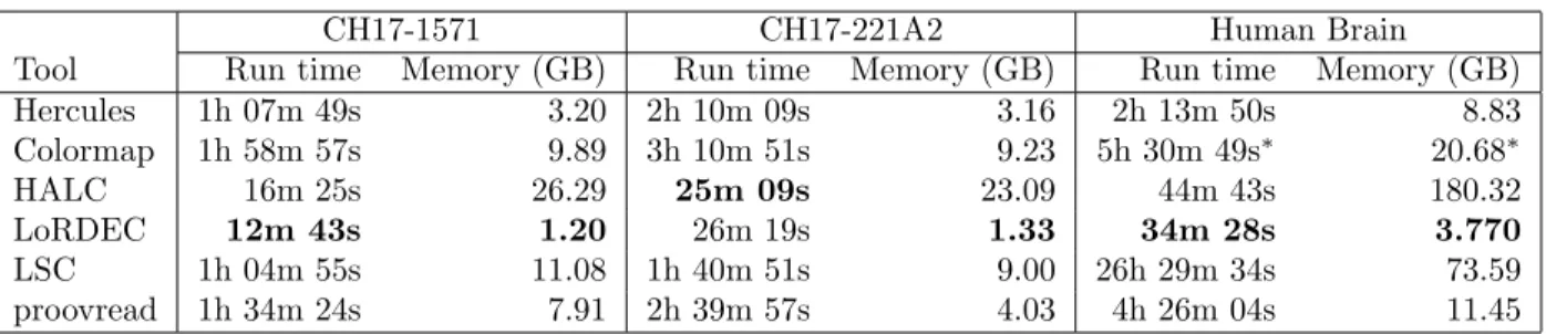
3.2.4 Run time and memory requirements . . . 31
A Data 42
List of Figures
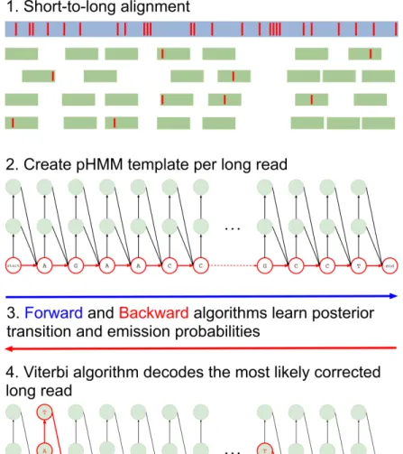
3.1 Overview of the Hercules algorithm. At the first step (1), short reads are aligned to long reads using an external tool. Here, red bars on the reads cor-respond to erroneous locations. Then, for each long read Hercules creates a pHMM with priors set according to the underlying technology as shown in (2). Using the starting positions of the aligned short reads, Forward-Backward al-gorithm learns posterior transition and emission probabilities. Finally, Viterbi algorithm finds the most likely path of transitions and emissions as highlighted with red colors in (3). The prefix and the suffix of the input long read in this example is “AGAACC...GCCT”. After correction, substring “AT” inserted right after the first “A”. Third “A” is changed to “T” and following two base-pairs are deleted. Note that deletion transitions are omitted other than this arrow, and only two insertion states are shown for clarity of the figure. On the suffix, a “T” is inserted and second to last base-pair is changed from “C” to “A”. . . 16 3.2 A small portion of the profile HMM built by Hercules. Here, two match
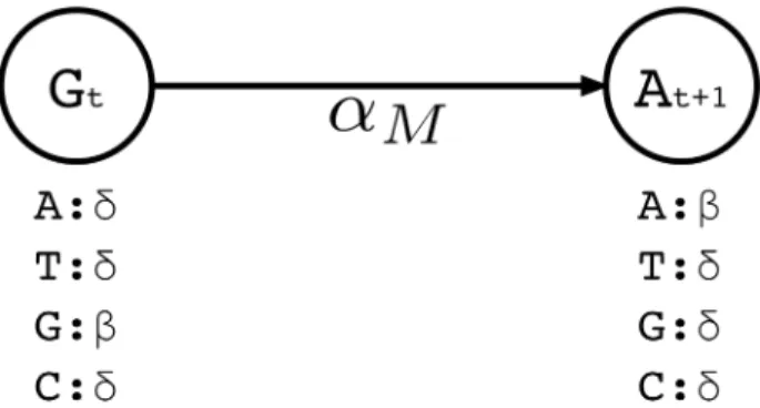
states are shown, where the corresponding long read includes G at location t, followed by nucleotide A at location t + 1. At state t, the emission probability for G is set to β, and emission probabilities for A, C, T are each set to the substitution error rate δ. Match transition probability between states t and t + 1 is initialized to αM. . . 20
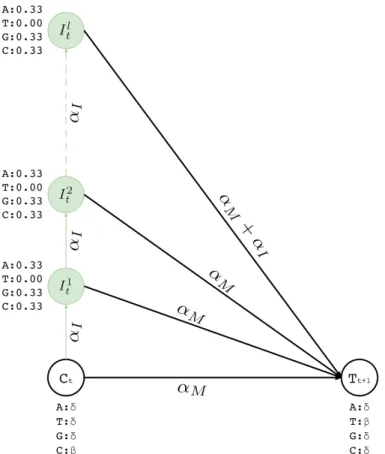
3.3 Insertion states for position t. Here we show two match states (Ct and Tt+1)
and l insertion states (It1. . . Itl). The number of insertion states limit the insertion length to at most l after basepair t of the corresponding long read. We also incorporate equal emission probabilities for all basepairs, except for the basepair represented by the corresponding match state t + 1 (T in this example). . . 22 3.4 Deletion transitions (red) in Hercules pHMM. Insertion states of position t
have the same deletion transitions with the match state of the same position, t. Any transition from position t to t + 1 + x removes x characters, skipping the match states between t and t + 1 + x, with ax
D probability, where 1 ≤ x ≤ k 23
3.5 Hercules profile HMM in full. Here we show the overall look at the complete graph that might be produced for a long read M where its tth character is
Mt and Mt ∈ {A, T, G, C} 1 ≤ t ≤ n and n is the length of the long read
M (i.e. |M | = n). In this example, there are n many match states and two insertion states for each match state. Only one character deletion is allowed at one transition because transitions may only skip one match state. . . 24
List of Tables
2.1 Summary of SNV, small indel, and deletion calls. . . 11
3.1 Summary of error correction . . . 29 3.2 Correction accuracy given high breadth of coverage (> 90%) in CH17-227A2. 30 3.3 Requirements of computational resources for all methods we compared. . . . 31
S1 List of data sets used in this study. . . 42 S2 Tools and their version numbers we used in this study. . . 43 S3 Summary of alignments of 1 million reads sampled from HG00096 in original
vs. shuffled order. . . 43 S4 Summary of scatter/gather based parallel read mapping of 1 million reads
using BWA-MEM. . . 44 S5 Summary of multithreaded read mapping of ∼49 million reads using
BWA-MEM. . . 44 S6 Summary of read mapping of the HG00096 genome in both original and
shuf-fled order using BWA-MEM. . . 44 S7 Summary of HaplotypeCaller call sets. . . 45
S8 Summary of UnifiedGenotyper call sets. . . 46
S9 Summary of FreeBayes call sets. . . 47
S10 Summary of SAMtools call sets. . . 48
S11 Summary of Platypus call sets. . . 49
S12 Summary of DELLY call sets (deletions). . . 50
S13 Summary of DELLY call sets (tandem duplications). . . 51
S14 Summary of DELLY call sets (inversions). . . 52
S15 Summary of DELLY call sets (translocations). . . 53
S16 Summary of Genome STRiP call sets (deletions). . . 54
S17 Summary of LUMPY call sets (deletions, chromosome 3 only). . . 54
S18 Summary of HaplotypeCaller call sets using the same BAM file twice. . . . 55
S19 Summary of UnifiedGenotyper call sets using the same BAM file twice. . . . 56
S20 Summary of Freebayes call sets using the same BAM file twice. . . 57
S21 Summary of SAMtools call sets using the same BAM file twice. . . 58
S22 Summary of Platypus call sets using the same BAM file twice. . . 59
S23 Summary of DELLY call sets using the same BAM file twice (deletions). . . 60
S24 Summary of DELLY call sets using the same BAM file twice (tandem dupli-cations). . . 61
S26 Summary of DELLY call sets using the same BAM file twice (translocations). 63 S27 Summary of Genome STRiP call sets using the same BAM file twice
(dele-tions). . . 64 S28 Summary of LUMPY call sets using the same BAM file twice (deletions,
chro-mosome 3 only). . . 64 S29 Summary of HaplotypeCaller call sets from 12 WES data sets using the same
BAM file twice. . . 65 S30 Performance of callers compared to 1000 Genomes OMNI SNP chip using the
same samples. . . 65 S31 Performance of callers compared to 1000 Genomes call set using the same
samples. . . 66 S32 Correction accuracy given high breadth of coverage (> 90%) in CH17-157L1. 66 S33 Effects of sequence coverage on correction accuracy for the CH17-157L1 BAC
Chapter 1
Introduction
The advancements in Next Generation Sequencing (NGS) technologies have increased the demand on producing genome sequence data for many research questions, and prompted pilot projects to test its power in clinical settings [1]. Any “medical test” to be reliably used in the clinic has to be proven to be both accurate and reproducible. However, the fast-evolving nature of NGS technologies make it difficult to achieve full reproducibility to generate essentially same data using the same DNA resources. NGS technologies suffer from two fundamental limitations. First and foremost, no platform is yet able generate a chromosome-long read. Average read length ranges from 100 bp to 10 Kbp depending on the platform. Second, reads are not error-free. The most ubiquitous platform, Illumina, produces the most accurate (<0.1% error rate), yet the shortest (100-150 bp) reads. Short read lengths present challenges in accurate and reproducible analyses [2, 3], as well as in building reliable assemblies [4, 5, 6]. On the other hand, Pacific Biosciences Single Molecule, Real-Time (SMRT) sequencing technology is capable of producing reads approximately 10 kbp-long on average with a substantially higher (∼15%) error rate [7]. Similarly, Oxford Nanopore Technologies (ONT) platform can generate longer reads (up to ∼900 Kbp) with the price of an even higher error rate (>20%) [8].
In Chapter 2, we first showed that resequencing the same DNA library with the same model NGS instrument twice and analyzing the data with the same algorithms may lead to different variation call sets [9]. There may be multiple reasons for this effect, such as
degradation of DNA between two sequencing experiments, signal processing and base calling errors during sequencing, or different GC biases introduced while making sequencing libraries from the same DNA [9].
Aside from the potential problems in the “wet lab” side, there may be additional com-plications in the “dry lab” analysis due to alignment errors and ambiguities due to genomic repeats. The repetitive nature of the human genome causes ambiguity in read mapping when the read length is short [2]. A 100 bp read generated by the Illumina platform may align to hundreds of genome locations with similar edit distance. The BWA-MEM [10] mapper’s approach to handle such ambiguity is randomly selecting one location, and assigning the mapping quality to zero to inform the variant calling algorithms that the alignment may not be accurate.
Although many algorithms exist for NGS data analysis, only a handful of computational pipelines for read mapping and variant calling may be considered as “standard” such as those that are commonly used in large scale genome projects (i.e. the 1000 Genomes Project [11]). For example, to discover and genotype variants using Illumina data, first the reads are mapped to reference genome assembly using BWA-MEM [10], Bowtie [12], or a simi-lar tool [13, 14] then the alignment files are processed using SAMtools [15] and Picard1, and finally the single nucleotide variants (SNV) and indels are predicted and filtered using GATK [16], Platypus [17], or Freebayes [18]. Structural variation (SV) discovery is even more challenging as exemplified by the 1000 Genomes Project [11, 19], where more than 20 algorithms were used to characterize SVs.
Recently, the Genome in a Bottle Project [20] was started to set standards for accu-rate NGS data analysis for both research and clinical uses by addressing the differences in detection performances of different algorithms and different sequencing platforms.
We investigated whether some of the commonly used variant discovery algorithms make use of the mapping quality information, and how they react to genomic repeats. Briefly, we aligned two whole genome shotgun (WGS) data sets, one low and one high coverage genome sequenced as part of the 1000 Genomes Project [11] to the human reference genome (GRCh37) twice using the same parameters. In the second mapping, we shuffled the order
of reads to make sure that the same random numbers are not used for the same reads. We then generated two SNV and indel call sets each from each genome.
We observed substantial differences in the call sets generated by all of the variant discovery tools we tested except VariationHunter/ CommonLAW. However, VariationHunter explicitly requires a deterministic read mapper, therefore we removed it from further comparisons. GATK’s HaplotypeCaller showed discordancies of 1.06% to 1.7% in SNV/indel call sets, where Freebayes showed the most concordancy (up to 99.2%). Genome STRiP showed the greatest discrepancy in structural variation calls (up to 25%). Our results raise questions about reproducibility of callsets generated with several commonly used genomic variation discovery tools.
Our discovery on reproducibility issues of DNA sequencing data suggests that it becomes harder to achieve reproducibility when repeats start to occur frequently. Short reads are vulnerable to repeats as the probability of mapping to a same location with the same edit distance is always higher than that of long reads. This ambiguity (1) raises questions about analyses and results that are produced after short read mapping and (2) increases time com-plexity of a short read mapping where the long read mapping of the same DNA sample is less time consuming [21]. However, the challenge of using long reads is much more obvious that long sequencing platforms introduce at least 15% error within long reads that they produce [7, 8]. Complementary strengths and weaknesses of these platforms make it attractive to use them in harmony, i.e. merging the advantage of the longer reads generated by PacBio and ONT platforms with the accuracy of Illumina. Arguably, one can achieve high basepair accuracy using only PacBio or ONT reads, if the sequence coverage is sufficiently high [22]. However, the relatively higher costs associated with long read platforms make this approach prohibitive. Therefore, it is still more feasible to correct the errors in long reads using more accurate short reads in a hybrid manner.
There are two major hybrid approaches for long read error correction. First approach starts with aligning short reads onto long reads generated from the same sample, implemented by several tools such as PacBioToCA [23], LSC [24], proovread [25], and Colormap [26]. Leveraging the relatively higher coverage and accuracy of short reads, these algorithms fix the errors in long reads by calculating a consensus of the short reads over the same segment of the nucleic acid sequence. The second approach aligns long reads over a de Bruijn graph
constructed using short reads, and the k-mers on the de Bruijn graph that are connected with a long read are then merged into a new, corrected form of the long read. Examples of this approach are LoRDEC [27], Jabba [28], HALC [29], and LoRMA [30].
The alignment based approach is highly dependent on the performance of the aligner. Therefore, accuracy, running time, and memory usage of an aligner will directly affect the performance of the downstream correction tool. The use of de Bruijn graphs eliminates the dependence on external aligners, and implicitly moves the consensus calculation step into the graph construction. However, even with the very low error rate in short reads and the use of shorter k-mers when building the graph, the resulting de Bruijn graph may contain bulges and tips, that are typically treated as errors and removed [31]. Accurate removal of such graph elements depend on the availability of high coverage data to be able to confidently discriminate real edges from the ones caused by erroneous k-mers [32, 33]. Therefore, performance of de Bruijn graph based methods depends on high sequence coverage.
Here, in Chapter 3, we introduce a new alignment-based hybrid error correction algorithm, Hercules [34], to improve basepair accuracy of long reads. Hercules is the first machine learning-based long read error correction algorithm. The main advantage of Hercules over other alignment-based tools is the novel use of profile hidden Markov models (dubbed profile HMM or pHMM). Hercules models each long and erroneous read as a template profile HMM. It uses short reads as observations to train the model via Forward-Backward algorithm [35], and learns posterior transition and emission probabilities. Finally, Hercules decodes the most probable sequence for each profile HMM using Viterbi algorithm [36]. Profile HMMs are first popularized by the HMMER alignment tool for protein families [37] and are used to calculate the likelihood of a protein being a member of a family. To the best of our knowledge, this is the first use of a profile HMM as template with the goal of learning the posterior probability distributions.
All alignment-based methods in the literature, (i) are dependent on the aligner’s full CIGAR string for each basepair to correct, (ii) have to perform majority voting to resolve discrepancies among short reads, and (iii) assume all error types (i.e., deletion) are equally likely to happen. Whereas, Hercules only takes the starting positions of the aligned short reads from the aligner, which minimizes the dependency on the aligner. Then, starting from
that position, it sequentially and probabilistically accounts for the evidence provided per short read, instead of just independently using majority voting per base-pair. Finally, prior probabilities for error types can be configured based on the error profile of the platform to be processed. As prior probabilities are not uniform, the algorithm is better positioned to predict the posterior outcome. Thus, it can also distinguish long read technologies.
We tested Hercules on the following datasets: (i) two BAC clones of complex regions of human chromosome 17, namely, CH17-157L1 and CH17-227A2 [7], and (ii) human brain cerebellum polyA RNA-seq data that LSC provides [24]. As the ground truth, (i) for BAC clones, we used finished assemblies generated from Sanger sequencing data from the same samples and (ii) for human brain data we used GRCh38 assembly. We show that Hercules-corrected reads has the highest mapping rate among all competing algorithms. We report ∼20% improvement over the closest de Bruijn based method, ∼2% improvement over the closest alignment-based method, and ∼30% improvement over the original version of long reads. We also show that, should long reads have high short read breadth of coverage provided by the aligner (i.e., 90%), Hercules outputs the largest set of most accurate reads (i.e., ≥95% accuracy).
Chapter 2
Effects of read length and genomic
repeats on the reproducibility of
genomic analyses
2.1
Methods
2.1.1
Data acquisition
We downloaded both whole genome and whole exome sequencing data sets from the 1000 Genomes Project [11] FTP server.
2.1.2
Read mapping, shuffling, and BAM file processing
We used Bowtie [12], RazerS3 [14], and BWA-MEM [10], and mrFAST [13] (Table S2) to align the reads generated by the Illumina platform to human reference genome (GRCh37) using default options. For testing the effects of read order, we randomly shuffled the reads in the FASTQ file using an in-house program, while keeping the relative order of read pairs
intact. The reason for reshuffling the reads is the following. In our small scale test, we noticed that BWA-MEM uses the same pseudorandom number generator seed in all mapping experiments. This causes the same ambiguously mapping read to be randomly assigned to the same position when the read order is intact. However, when we shuffle the reads, the random number that corresponds to the read changes, causing it to be placed to another random location. Note that, the DNA molecules are hybridized randomly to the oligos on the flow cell, thus, our read randomization simulates the randomness in cluster generation. Next, we used SAMtools [15] to merge, sort, and index BAM files, and Picard1 to remove PCR duplicates (MarkDuplicates). We then followed the GATK’s “best practices” guide [38] to realign around indels (RealignerTargetCreator and IndelRealigner) and recalibrate base quality values (BaseRecalibrator). We used the resulting BAM files for SNV, indel, and SV calling. The names and version numbers of the tools we used are listed in Table S2.
2.1.3
SNVs and indels
We used GATK HaplotypeCaller [16], SAMtools [15], Freebayes [18], and Platypus [17] to characterize SNV and indels. We followed the developers’ recommendations and default parameters for all variant calling tools, including potential false positive filters. Specifically, we used both Variant Quality Score Recalibrator and SnpCluster methods to filter out false positives in GATK call sets, and for other tools we required a variant quality of at least 30. For GATK, we used the GATK Resource Bundle version 2.8 as the reference genome and its annotations, and variant score recalibration training material.
2.1.4
Structural variation
For structural variation discovery using the BWA-generated BAM files, we tested the re-producibility of the calls produced by DELLY [39], LUMPY [40], Genome STRiP [41], and VariationHunter/ CommonLAW [42, 43]. We note that VariationHunter explicitly remaps reads to the reference genome using mrFAST, which is a deterministic mapper, therefore we removed it from further comparisons. We used default parameters for each tool and followed recommendations in relative documentations.
2.1.5
Variant annotation and comparison
We downloaded the coordinates for segmental duplications, genes, coding exons, and common repeats from the UCSC Genome Browser [44]. We then used the BEDtools suite [45] and standard UNIX tools to calculate the discrepancies among the call sets and their underlying sequence annotations.
2.2
Results
2.2.1
Data and tools
We downloaded two WGS data sets, one at low coverage (∼5X, HG00096) and one at high coverage (∼ 44X, HG02107), and 12 WES data sets with coverage ranging from 120X to 656X from the 1000 Genomes Project [11] (Table S1). We tested the behaviors of three different read mappers, four SNV/indel callers, and three SV characterization algorithms (Table S2, Methods).
2.2.2
Small scale test for ambiguous mapping
We first sub sampled 1 million reads from HG00096, and mapped it to the human reference genome (GRCh37) using Bowtie, RazerS3, mrFAST, and BWA-MEM [10]. Next, we ran-domly shuffled the reads in the FASTQ file (Methods), and remapped the reordered reads to GRCh37 using the same tools. The read randomization simulates the random nature of DNA hybridization on the flow cell. We confirmed that mrFAST and Bowtie generated the same alignments, as described in their respective documentations, where BWA-MEM mapped several reads to different locations due to placing such reads to random locations (Table S3).
2.2.3
Read mapping in parallel
Due to the large number of reads generated by NGS platforms, it is a common practice to use scatter/gather operations (or, its implementation using the MapReduce framework) to distribute the work load to large number of CPUs in a cluster. This approach leverages the embarrassingly parallel nature of read mapping, where the FASTQ files that typically contain >50 million reads are divided into “chunks” with just 1-2 million reads per file, the reads in each chunk are mapped separately, and the resulting BAM files are combined. Reasoning from our observation of different random placements of ambiguous reads when the reads are shuffled, we employed the scatter/gather method to map 1 million reads twice, using different chunk sizes. In this experiment we divided the reads into chunks of 50,000 and 100,000 read pairs, mapped them using BWA-MEM, and observed mapping discordance ratios similar to that of random shuffling (2.1%, Table S4). We also observed less pronounced differences in read mapping when different number of threads are used for the same FASTQ file (0.05%, Table S5).
2.2.4
WGS analysis
We then repeated the same mapping strategy to the full versions of all data sets we down-loaded, but we mapped using only BWA-MEM, since we observed the other mappers to be deterministic based on the small scale test. We also investigated BWA-MEM’s behavior of random placements using the HG00096 genome, and interestingly, although BWA-MEM reported zero mapping qualities for most of the discrepant read mappings (∼97%), it also assigned high MAPQ values (≥30) for a fraction of them (∼0.75%; Table S6).
2.2.5
Single nucleotide variants and indels
We used GATK’s HaplotypeCaller, Freebayes, Platypus, and SAMtools to characterize SNVs and indels within the HG00096 and HG02107 genomes using recommended parameters for each tool (Methods). We did not evaluate GATK UnifiedGenotyper since it is deprecated by its developers. We then compared each call set generated by the same tools using the
reads in original vs. shuffled order using BEDtools [45], and found up to 1.70% of variants to be called in one alignment of the same data but not in the other (Table 2.1). Next, we investigated the underlying sequence context of the SNVs and indels differently detected using the same tools with two different alignments (i.e. original vs shuffled order). As expected, 72- to 80% of the discrepant calls were found within common repeats and segmental duplications (Tables S7,S9,S10,S11). In most genomic analysis studies duplications and repeats are removed from analyses; however, in this study we observed discrepancies in functionally important regions (i.e. coding exons). For example, 253-1,249 SNVs that were called from one alignment but not another map to coding exons (Table S7). Furthermore, 1,543 of the 1,884 (81.9%) discordant exonic SNVs predicted by GATK HaplotypeCaller (either original or shuffled order, non-reduntant total) did not intersect with any common repeats or segmental duplications.
Freebayes, Platypus, and SAMtools predictions were more reproducible, as >98.5% of the calls were identical, and the number of exonic discrepant SNV calls were substantially lower than that of GATK’s (Tables S9,S10,S11).
2.2.6
Structural variation
Next, we analyzed the deletion calls predicted using DELLY, LUMPY, and Genome STRiP. All three SV detection tools we tested showed 1.55%- to 25.01% difference in call sets us-ing the original vs. shuffled order read data sets (Table 2.1). Similarly, the discrepancies were mostly found within repeats and duplications, however, only a couple of deletion calls intersected with coding exons (Tables S12, S16, S17).
Using DELLY we predicted ∼3% of deletion, ∼4% of tandem duplication, ∼6% of in-version, and ∼3.6% of translocation calls to be specific to a single alignment, and >91% of these differences intersected with common repeats. Owing to the difficulties in predicting these types of SVs, more discrepant calls intersected with functionally important regions (i.e. genes and coding exons; Tables S13,S14,S15).
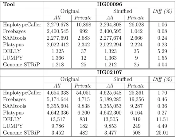
Table 2.1: Summary of SNV, small indel, and deletion calls.
Tool HG00096
Original Shuffled Diff (%)
All Private All Private
HaplotypeCaller 2,279,678 10,898 2,294,808 26,028 1.06 Freebayes 2,400,545 992 2,400,595 1,042 0.08 SAMtools 2,277,691 2,683 2,277,674 2,666 0.24 Platypus 2,022,412 2,342 2,022,294 2,224 0.23 DELLY 1,325 37 1,323 35 5.29 LUMPY 1,366 12 1,363 9 1.55 Genome STRiP 1,218 25 1,212 25 4.04 HG02107
Original Shuffled Diff (%)
All Private All Private
HaplotypeCaller 4,654,338 54,051 4,625,648 25,361 1.70 Freebayes 5,174,644 4,715 5,189,285 19,356 0.46 SAMtools 5,355,604 9,838 5,355,053 9,287 0.36 Platypus 4,642,336 6,200 4,642,300 6,164 0.27 DELLY 13,517 831 13,505 819 11.51 LUMPY 9,786 182 9,853 249 4.49 Genome STRiP 3,452 482 3,477 508 25.01
We list the number of SNV, small indel, and deletion calls in the genomes of HG00096 and HG02107 characterized by different tools using the reads in the original (i.e. as released by 1000 Genomes Project), and shuffled order. Calls that are specific to one order of reads are listed as Private. The difference percentage is calculated as the total number of Private calls divided by the number of calls in the union set (i.e. |(O\S) ∪ (S\O)||O∪S| , O: original, S: shuffled).
2.2.7
Reusing the same alignments
More interestingly, when we ran GATK’s HaplotypeCaller on the same BAM file twice we observed discrepant calls similar to using two different BAM files generated from original vs shuffled read order (Table S18). Other tools produced no discrepancies (Tables S20-S28). Detailed analysis of these discordancies revealed that 21,497 of the 21,510 (>99.9%) “second-run specific” HaplotypeCaller calls were initially found in the first “second-run, however filtered in the Variant Quality Score Recalibration (VQSR) step. Similarly, 10,631 of the 10,646 “first-run specific” HaplotypeCaller calls were eliminated by VQSR in the second run. We
then performed a line-by-line analysis in such calls, and found that the VQSLOD score was calculated differently, although the training data was the same in both runs. We speculate that this is due to the random sampling of the training data to reduce computational burden1. We then confirmed our observation by rerunning the VQSR filter on one of the VCF files five times. Each iteration of the VQSR filtering generated a different set of VQSLOD values, causing different variants to be filtered.
2.2.8
Exome analysis
Finally, we tested the effect of discordant call sets generated by GATK even with the same alignment files using 12 whole exome shotgun sequence (WES) data sets from the 1000 Genomes Project (Table S1). We followed the same alignment, post-processing for the WES data sets. We then generated two call sets each using HaplotypeCaller on the same BAM files, followed with VQSR filtering. In this experiment, we used the multi-sample calling options. HaplotypeCaller produced discordant calls at 1-to 3% rate (Tables S18,S29).
2.3
Discussion
The introduction of NGS platforms quickly revolutionized the way we do biological research[46, 47]. Furthermore, NGS technology already started to make impact on human health in the form of personalized medicine through clinical sequencing [1], breast cancer subtype detection [48], and small molecule drug target site identification [49]. However, both sequencing technologies themselves [9], and the computational tools are still far from being mature in terms of accuracy [50, 51]. The complexity and repetitive nature of human genomes introduce further challenges for reliable characterization of genomic variants [2].
In this chapter, we documented the effects of different approaches to handle ambiguities in read mapping due to genomic repeats. We focused on more widely used computational tools for read mapping and variant calling, and observed that random placement of ambiguously
1
This random subsampling can be seen in the GATK code VariantDataManager.java at https://github. com/broadgsa/gatk-protected/ (commit ID: 8ea4dcab8d78e7a7d573fcdc519bd0947a875c06, line 255)
mapping reads have an effect on called variants. Although discordancies within repeats are less of a concern due to their relatively negligible effects to phenotype, we also discovered hundreds to thousands variants differently detected within coding exons. HaplotypeCaller showed the most discrepancies, where the discordant calls were less pronounced in Freebayes and Platypus results. Using the same alignments twice, we found that the callers themselves are deterministic, however, they return different call sets when the same data is remapped. Interestingly, we observed differences in call sets generated using HaplotypeCaller even when the same alignments and variant filtration training data sets were provided. Although we could not fully characterize the reasons of this observation with GATK, since HaplotypeCaller algorithm is yet unpublished, we observed that the differences were mainly due to differences in calculation of the VQSLOD score by the VQSR filter (Results). Therefore, a second source of randomness we observed is within the training step of the VQSR filter, which is specific to GATK.
2.3.1
Recommendations
We, point out that randomized algorithms may achieve better accuracy in practice, albeit without 100% reproducibility. Full reproducibility could only be achieved through using deterministic methods. Therefore, for full reproducibility, we recommend to opt for a deter-ministic read mapper such as Bowtie, mrFAST, etc., and a deterdeter-ministic variant caller, such as Platypus or Freebayes for SNV and indels. We note that all SV calling algorithms we surveyed in our study are deterministic algorithms, therefore the SV call sets can be fully reproducible when they are used together with a deterministic mapper. Another approach may be more strict filtering of variants that map to repeats and duplications, however this may result in lower detection power in functionally important duplicated genes such as the MHC and KIR loci. It may be possible to work around the GATK’s VQSLOD calculation problem outlined above by setting the maxNumTrainingData parameter and other downsam-pling parameters to high values, however, we recommend disabling these randomizations by default to be a better practice for uninformed users. In our tests, changing only the maxNumTrainingData parameter did not fully resolve the variant filtration problem, which points that there may be other downsampling and/or randomization step within the VQSR filter.
2.3.2
Conclusion
Mapping short reads to repetitive regions accurately still remains an open problem [2]. Bowtie and mrFAST use edit distance and paired-end span distance to deterministically assign a single “best” map location to ambiguously mapping reads, where BWA-MEM se-lects a random map location all mapping properties are calculated the same. BWA-MEM assigns a zero mapping quality to such randomly selected alignments. This approach is still valid since it informs the downstream analysis tools for problematic alignments, however, as we have documented in this manuscript, several variant discovery tools do not fully utilize this information. Complete analysis of the reasons for these discrepancies may warrant code inspection and full disclosure of every algorithmic detail.
The differences in call sets we observed in this study have similar accuracy when compared to 1000 Genomes data (Supplementary Table S30, S31). In addition a recent study did not find any significant difference between deterministic and non-deterministic mappers in terms of accuracy [52]. It is still expected to have differences between different algorithms and/or parameters, but obtaining different results should not be due to the order of independently generated reads in the input file. We may simply count these discordancies as false positives and negatives, and such discordancies may not have any adverse effects in practice, however, we argue that computational predictions should not be affected by luck, and inaccuracies in computational results should be deterministic so they can be better understood and characterized. We are in exciting times in biological research thanks to the development of NGS technologies. However, under the shining lights of the discoveries we make in this “big biology” revolution, it can be easy to overlook that the methods matter. No genomic variant characterization algorithm achieves 100% accuracy yet, even with simulation data, but it is only possible to analyze and understand the shortcomings of deterministic algorithms, and impossible to fully understand how an algorithm performs if it makes random choices.
Chapter 3
Error correction for long reads
3.1
Methods
3.1.1
Overview of Hercules
Hercules [34] corrects errors (insertions, deletions, and substitutions) present in long read sequencing platforms such as PacBio SMRT [53] and Oxford Nanopore Technologies [8], using reads from a more accurate orthogonal sequencing platform, such as Illumina [54]. We refer to reads from the former are referred as “long reads” and the latter as “short reads” in the remainder of this chapter. The algorithm starts with preprocessing the data and obtains the short-to-long read alignment. Then, for each long read, Hercules constructs a pHMM template using the error profile of the underlying platform as priors. It then uses the Forward-Backward algorithm to learn the posterior transition/emission probabilities, and finally, uses the Viterbi algorithm to decode the pHMM to output the corrected long read (Figure 3.1).
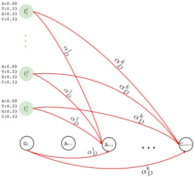
Figure 3.1: Overview of the Hercules algorithm. At the first step (1), short reads are aligned to long reads using an external tool. Here, red bars on the reads correspond to erroneous locations. Then, for each long read Hercules creates a pHMM with priors set according to the underlying technology as shown in (2). Using the starting positions of the aligned short reads, Forward-Backward algorithm learns posterior transition and emission probabilities. Finally, Viterbi algorithm finds the most likely path of transitions and emissions as highlighted with red colors in (3). The prefix and the suffix of the input long read in this example is “AGAACC...GCCT”. After correction, substring “AT” inserted right after the first “A”. Third “A” is changed to “T” and following two base-pairs are deleted. Note that deletion transitions are omitted other than this arrow, and only two insertion states are shown for clarity of the figure. On the suffix, a “T” is inserted and second to last base-pair is changed from “C” to “A”.
3.1.2
Preprocessing
3.1.2.1 Compression
Similar to the approach of LSC [24], Hercules starts with compressing both short and long reads using a run-length encoding scheme. That is, it compresses repeating base-pairs to a single base-pair (e.g., AAACTGGGAC → ACTGAC). This is because PacBio and ONT platforms are known to produce erroneous homopolymer runs, i.e. consecutive bases may be erroneously repeated [53, 8], which affects the short read alignment performance drastically. Hercules, then, recalculates the original positions based on the original long reads. Even though this option is performed by default, it is still possible to skip the compression phase. Hercules obtains 3-fold increase in the most accurate reads (i.e., >95% accuracy) when compression phase is enabled. Doing so, the number of aligned reads also increases by ∼30%.
3.1.2.2 Short Read Filtering
After the step described above, the nominal length of some compressed reads may be sub-stantially shortened. This would in turn cause such reads to be ambiguously aligned to the long reads, which is already a common problem in short read sequencing due to repeats [2, 3]. To reduce this burden, Hercules removes any compressed short read, if its number of non-N characters is less than a specified threshold (set to 40 by default). In addition to PCR and optical duplicates inherent in short read data, it is also highly likely that compres-sion step will generate new duplicate sequences. These duplicate reads will not carry any extra information for correcting the long reads. Therefore, after compression, Hercules may remove these duplicates using a Bloom filter with 0.0001 false positive rate, keeping only a single read as the representative of the group. Duplicate removal is an optional phase, and we do not remove duplicates by default.
3.1.2.3 Alignment and Decompression
Hercules is an alignment-based error correction tool. It outsources the alignment process to a third party aligner. It is compatible with any aligner that provides output in SAM format [15]. However, we suggest mappers that can report multiple possible alignments such as Bowtie2 [55] as we would prefer to cover most of the long read with short reads. Even though this might cause incorrect mappings, Hercules is able to probabilistically downplay the importance of such reads during the learning stage given sufficient short read depth. Hercules also assumes that the resulting alignment file is sorted. Thus, the file in SAM/BAM format must be coordinate sorted in order to ensure a proper correction with Hercules. Alignments are calculated using either compressed or original long and short reads (those that pass filtering step for the latter) as described in previous sections. After receiving the alignment positions from the aligner, Hercules decompresses both short and long reads and recalculates alignment start locations.
All other alignment-based error correction methods in the literature use the CIGAR string provided by the aligner. CIGAR string specifies where each basepair of the short read is mapped on the long read and where insertions and deletions have occurred. Then, per base-pair on the long read, they perform a majority voting among covering short reads. Hence, learning of correct basepairs is actually performed by the aligner, which makes the performance of such tools fully dependent on the aligner choice. Even though, Hercules is also an alignment-based method, the only information it receives from the aligner is the starting position of the mapping. Forward algorithm learns posterior probabilities starting from that position and it can go beyond the covered region. Thus, despite using the starting point information from the aligner, the algorithm can decide the short read is aligned after that point and also that the alignment is essentially different than what is claimed by the aligner in the CIGAR string. This minimizes the dependency of the algorithm on the aligner and makes Hercules the first alignment-based approach to reclaim the consensus learning procedure from the aligner.
3.1.3
The Profile HMM Structure
Hercules models each long read as a pHMM. In a traditional profile HMM [37], there are three types of states: deletion, insertion and match (mismatch) states. The aim is to represent a family of proteins (amino acid sequences) and then to use it to decide if an unknown protein is likely to be generated from this model (family). Our goal in representing a long read as a template pHMM is entirely different. For the first time, we use short reads that we know are generated from the source (e.g., same section of RNA/DNA), to update the model (not the topology but the transition and emission probabilities). So, the goal in the standard application is to calculate the likelihood of a given sequence, whereas in our application there is no given sequence. We would like to calculate the most likely sequence the model would produce, among all possible sequences that can be produced using the letters in the alphabet Σ. This requires us to impose some restrictions on the standard pHMM concept. First, we remove the self loop over insertion states. Instead, our model has multiple insertions states per position (basepair) on the long read. The number of insertion states is an input the algorithm. Second, we substitute deletion states with deletion transitions. The number of possible consecutive basepairs that can be deleted is an input parameter to the algorithm as well.
After we construct the model, we use the error profile of the underlying technology to initialize the prior transition and emission probabilities. Hercules first learns posterior tran-sition and emission probabilities of each “long read profile HMM” using short reads that align to the corresponding long read. Then, it decodes the pHMM using the Viterbi algo-rithm [36] to generate the most probable (i.e. corrected, or consensus) version of the long read.
It should be noted that the meanings of insertion and deletion is reversed in the context of the pHMM. That is, an insertion state would insert a basepair into the erroneous long read. However, this means that the original long read did not have that nucleotide and had a deletion in that position. Same principle also applies to deletions.
Next, we first define the structure of the model (states and transitions) and explain how we handle different types of errors (i.e. substitutions, deletions, and insertions). We, then, describe the training process. Finally, we explain how Hercules decodes the model and
Figure 3.2: A small portion of the profile HMM built by Hercules. Here, two match states are shown, where the corresponding long read includes G at location t, followed by nucleotide A at location t + 1. At state t, the emission probability for G is set to β, and emission probabilities for A, C, T are each set to the substitution error rate δ. Match transition probability between states t and t + 1 is initialized to αM.
generates the consensus sequence.
3.1.3.1 Match States
Similar to traditional pHMM, we represent each basepair in the long read by a match state. There are four emission possibilities (Σ = {A, C, G, T }). The basepair that is observed in the uncorrected long read for that position t is initialized with the highest emission probability (β), while the probabilities for emitting the other three basepairs are set to the expected substitution error rate for the long read sequencing technology (δ) (Note that β δ and β + 3δ = 1).
We then set transition probabilities between consecutive match states t and t+1 as “match transitions” with probability αM. Figure 3.2 exemplifies a small portion of the profile HMM
that shows only the match states and match transitions. From a match state at position t, there are also transitions to (i) the first insertion state at position t (I1
t), and (ii) to all
match states at positions t + 1 + x where 1 ≤ x ≤ k and k determines the number of possible deletions.
3.1.3.2 Insertion States
Insertion states have self-loop transitions in standard profile HMMs to allow for multiple insertions at the same site, which creates ambiguity for error correction for two reasons. First, self-loops do not explicitly specify the maximum number of insertions. Thus, it is not possible predetermine how many times that a particular self-loop will be followed while decoding. Second, each iteration over the loop has to emit the same basepair. Since decoding phase prefers most probable basepair at each state, it is not possible for a standard profile HMM to choose different nucleotides from the same insertion state.
Instead of a single insertion state with a self loop per basepair in the long read, we con-struct l multiple insertion states for every match state at position t (e.g., I1
t . . . Itl). We
replace self-loops with transitions between consecutive insertion states (Itj. . . Itj+1) for posi-tion t (see Figure 3.3). The probability for each of such transiposi-tions is αI and the number of
insertion states per position l determines the maximum number of allowed insertions between two match states, which are set through user-specified parameters. All insertion states at position t have transitions to the match state at positions t + 1 (end states is also considered as a match state). For I1
t . . . I l−1
t the probability of those transitions are αM, and for Itl, it
is αM + αI. All those states also have transitions to all match states at positions t + 1 + x
where 1 ≤ x ≤ k and k determines the number of possible deletions.
We also set emission probabilities for the insertion states and assume they are equally likely. However, for the insertion states at position t, we set the probability of emitting the nucleotide X ∈ Σ to zero, if X is the most likely nucleotide at the match state of position t+1. This makes the insertion more likely to happen at the last basepair of the homopolymer run. Otherwise, the likelihood of inserting a basepair is shared among all insertions states of the run, and it is less likely for any them to be selected during the decoding phase. All other basepairs have their emission probabilities set to 0.33 (i.e. |Σ|−11 )- see Figure 3.3.
3.1.3.3 Deletion Transitions
In standard pHMM, a deletion state needs to be visited to skip (delete) a basepair, which does do not emit any characters. However, as described in the following sections, calculation
Figure 3.3: Insertion states for position t. Here we show two match states (Ctand Tt+1) and
l insertion states (It1. . . Itl). The number of insertion states limit the insertion length to at most l after basepair t of the corresponding long read. We also incorporate equal emission probabilities for all basepairs, except for the basepair represented by the corresponding match state t + 1 (T in this example).
of the forward and backward probabilities for each state is based on the basepair of the short read considered at that time. This means at each step, the Forward-Backward algorithm consumes a basepair of the short read to account for the evidence the short read provides for that state. As deletion states do not consume any basepairs of the short read, this in turn results in an inflation on the number of possibilities to consider and substantially increases the computation time. In an extreme case, the short read implying its mapped region on the long read may be deleted entirely. Since we are using an external aligner, such extreme cases are unlikely. Thus, we model deletions as transitions, instead of having deletion states. In our model, a transitions to (1+x)-step away match states is established to delete x basepairs. As shown in Figure 3.4, match and insertion states at tth position have a transition to all
match states at positions t + 1 + x, where 1 ≤ x ≤ k and k is an input parameter determining maximum number of deletions per transition. We calculate the probability of a deletion of
Figure 3.4: Deletion transitions (red) in Hercules pHMM. Insertion states of position t have the same deletion transitions with the match state of the same position, t. Any transition from position t to t + 1 + x removes x characters, skipping the match states between t and t + 1 + x, with axD probability, where 1 ≤ x ≤ k
x basepairs, αx D, as shown in Equation 1. αxD = f k−xα del k−1 P j=0 fj 1 ≤ x ≤ k (1)
Equation 1 is a normalized version of a polynomial distribution where αdel is the overall
deletion probability (i.e. αdel = 1 − αM − αI), and f ∈ [1, ∞). As f value increases,
probabilities of further deletions decrease accordingly.
3.1.3.4 Training
An overall illustration of a complete pHMM for a long read of length n is shown in Figure 3.5 where (i) match states are labeled with Mt where M ∈ Σ, (ii) insertion states are labeled
with I1
t and It2, and (iii) deletion transitions for k = 1 are shown. Note that tth basepair of
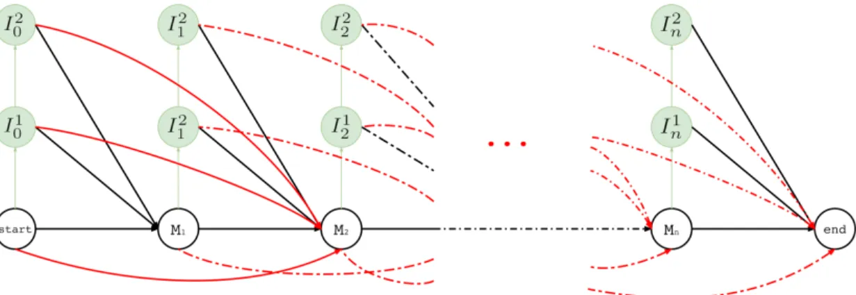
Figure 3.5: Hercules profile HMM in full. Here we show the overall look at the complete graph that might be produced for a long read M where its tthcharacter is M
tand Mt∈ {A, T, G, C}
1 ≤ t ≤ n and n is the length of the long read M (i.e. |M | = n). In this example, there are n many match states and two insertion states for each match state. Only one character deletion is allowed at one transition because transitions may only skip one match state.
deletion transitions from every state at tthposition to (t + 2)th match state where (t + 2) ≤ n. This example structure allows only one character deletion at one transition since it is only capable of skipping one match state.
Let the complete pHMM for a long read be the graph G(V, E). Per each mapped short read s, we extract a sub-graph Gs(Vs, Es). Here Gs corresponds to the covered region of the
long read with that short read. We train each Gs using the Forward-Backward algorithm
[35]. Hercules may not consider some of the short reads that align to same position in a long read to reduce computational burden. We provide max coverage, mc, option to only consider mc many number of short reads for a position during a correction, where mc = 20 by default. Short reads are selected based on their edit distance.
States that will be included in Vs are determined by several factors. First, assume that
s is aligned to start from the qth character of the long read. First, all match and insertion
states between positions [q − 1, q + m) are included, where m is the length of the short read. If there are insertion errors, deletion transitions might be followed which may require training phase to consider r more positions where r is a parameter to the algorithm, which is fixed to dm/3e. Thus all match and insertion states between [q + m, q + m + r) are also added. Finally, the match state at position q + m + r is also included (end state), and Mq−1
acts as the start state. Every transition Eij ∈ E connecting state i and state j are included
as described in previous subsections. For every pair of states, i ∈ Vs and j ∈ Vs, αij = 0 if
Eij 6∈ Es.
Let ei(s[t]) be the emission probability of the tthbasepair of s from state i. We recursively
calculate forward probabilities Ft(i), ∀i ∈ Vs, where 1 ≤ t ≤ m and F1(i) is the base case.
F1(j) = αstart−jej(s[1]) s.t. j ∈ Vs, Estart−j ∈ Es (2.1)
Ft(j) =
X
i∈Vs;Eij∈Es
Ft−1(i)αijej(s[t]) j ∈ Vs, 1 < t ≤ m (2.2)
The forward probability Ft(j) denotes the probability of being at state j having observed
t basepairs of s. All transitions that lead to state j contributes to the probability with (i) the forward probability of the origin state i calculated with the t − 1th basepair in s, multiplied by (ii) the probability of the transition from i to j, which is then multiplied by (iii) the probability of emitting s[t] from state j.
Backward probability Bt(j) is also calculated recursively as follows, for each state j ∈ Vs
where Bm(j) is the base case.
Bm(j) = αj−end j ∈ Vs, Ej−end∈ Es (3.1)
Bt(j) =
X
i∈Vs;Eij∈Es
αjiei(s[t + 1])Bt+1(i) j ∈ Vs, 1 ≤ t < m (3.2)
The backward probability Bt(i) denotes the probability of being at state j and then
observing the basepairs t + 1 to m from s. All outgoing transitions from state j to a destination state i contribute to this probability with (i) the backward probability of the state i with the t + 1th basepair of s, multiplied by (ii) the transition probability from the
state j to state i, which is then multiplied by (iii) the probability of i emitting the t + 1th basepair of s.
During calculations of both forward and backward probabilities, at each time step t, we only consider mf number of highest forward probabilities of the previous time step, t − 1. This significantly reduces that time required to calculate forward and backward probabilities, while ensuring not to miss any important information if mf value is chosen as we suggest in the next section.
After calculation of the forward and backward probabilities (expectation step), posterior transmission and emission probabilities are calculated (maximization step), as shown in equations 4 and 5, respectively.
ˆ ei(X) = m P t=1 Ft(i)Bt(i)(s[t] == X) m P t=1 Ft(i)Bt(i) ∀X ∈ Σ, ∀i ∈ Vs (4) ˆ αij = m−1 P t=1 αijej(s[t + 1])Ft(i)Bt+1(j) m−1 P t=1 P x∈Vs αixex(s[t + 1])Ft(i)Bt+1(x) ∀Eij ∈ Es (5)
As we explain above, updates of emission and transition probabilities are exclusive for each sub-graph Gs. Thus, there can be overlapping states and transitions that are updated within
multiple sub-graphs, independently using the prior probabilities. For such cases, updated values are averaged with respect to posterior probabilities from each subgraph. Uncovered regions keep prior transition and emission probabilities, and G is updated with the posterior emission and transmission probabilities.
3.1.3.5 Decoding
Decoding is the final process for the correction of a long read. It reads the updated complete graph, G, to decode the corrected version of a long read. For this purpose, we use the Viterbi algorithm [36] to decode the consensus sequence. We define the consensus sequence as the most likely sequence the pHMM produces after learning new parameters. The algorithm takes G for each long read and finds a path from the start state to the end state, which
yields the most likely transitions and emissions using a dynamic programming approach. For each state j, the algorithm calculates vt(j), which is the maximum marginal forward
probability j obtains from its predecessors when emitting the tth basepair of the corrected long read. It also keeps a back pointer, bt(j), which keeps track of the predecessor state i
that yields the vt(j) value. Similar to calculations of forward and backward probabilities,
we also consider mf many most likely Viterbi values from the previous time step, t − 1, to calculate vt(j).
Let ej ∈ Σ be the basepair that is most likely to be emitted from state j and T be
the length of the decoded sequence which is initially unknown. The algorithm recursively calculates v values for each position t of a decoded sequence as described in equations 6.1 and 6.3. The algorithm stops at iteration T∗ such that for the last iter iterations, the maximum value we have observed for v(end) cannot be improved - iter is a parameter and set to 100 by default. T is then set to t∗ such that vt∗(end) is the maximum among all
iterations 1 ≤ t ≤ T∗. 1. Initialization v1(j) = astart−jej ∀j ∈ V (6.1) b1(j) = start ∀j ∈ V (6.2) 2. Recursion vt(j) = max i∈V vt−1(i)αijej ∀j ∈ V, 1 < t ≤ T (6.3) bt(j) = argmax i∈V vt−1(i)αijej ∀j ∈ V, 1 < t ≤ T (6.4) 3. Termination vT(end) = max
i∈V vT(i)αi−end (6.5)
bT(end) = argmax i∈V
3.2
Results
3.2.1
Experimental setup
We implemented Hercules in C++ using the SeqAn library [56]. The source code is avail-able under the BSD 3-clause license at https://github.com/BilkentCompGen/Hercules. We compare our method against Colormap, HALC, LoRDEC, LSC, and proovread. We ran all tools on a server with 4 CPUs with a total of 56 cores (Intel Xeon E7-4850 2.20GHz), and 1 TB of main memory. We assigned 60 threads to all programs including Hercules.
We used Bowtie2 with the multi-mapping option enabled to align the reads, and then we sorted resulting alignment files using SAMtools [15]. For Hercules, we set our parameters as follows: max insertion length (l = 3), max deletion length (k = 10), match transition probability (aM = 0.75), insertion transition probability (aI = 0.20), deletion transition
probability (adel = 0.05), deletion transition probability distribution factor (f = 2.5), match
emission probability (β = 0.97), max coverage (mc = 1), max filter size (mf = 100). We ran all other programs with their default settings.
In our benchmarks we did not include the error correction tools that use another correc-tion tool internally such as LoRMA, which explicitly uses LoRDEC. Similarly, HALC also uses LoRDEC to refine its corrected reads. However, it is possible to turn off this option, therefore we benchmarked HALC without LoRDEC. We also exclude Jabba in our compar-isons because it only provides corrected fragments of long reads and clips the uncorrected prefix and suffixes, which results in shorter reads. All other methods consider the entire long read. Additionally, several error correction tools such as LSC and proovread do not report such reads that they could not correct. Others, however, such as Hercules, LoRDEC, and Colormap report both corrected and uncorrected reads, preserving the original number of reads. In order to make the results of all correction tools comparable, we re-insert the original versions of the discarded reads to LSC and proovread output. We ran Colormap with its additional option (OEA) that incorporates more refinements on a corrected read. We observed that there was no difference between running OEA option or not in terms of the accuracy of its resulting reads, although Colormap with OEA option required substantially higher run time.
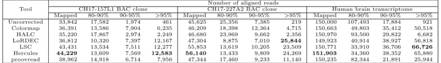
Table 3.1: Summary of error correction
Tool
Number of aligned reads
CH17-157L1 BAC clone CH17-227A2 BAC clone Human brain transcriptome Mapped 80-90% 90-95% >95% Mapped 80-90% 90-95% >95% Mapped 80-90% 90-95% >95% Uncorrected 33,842 17,582 1,974 461 45,625 25,356 7,385 219 150,000 107,493 17,884 921 Colormap 36,391 13,586 7,904 6,235 46,209 18,398 12,364 4,715 150,663 49,803 35,412 50,518 HALC 35,220 17,867 2,974 2,249 46,680 23,969 9,662 2,356 150,970 93,500 29,822 6,682 LoRDEC 36,812 10,320 7,397 12,167 47,304 8,875 7,010 25,844 149,923 40,914 38,927 56,818 LSC 43,431 13,534 7,511 12,277 55,853 13,619 10,205 23,509 150,771 33,910 36,706 66,726 Hercules 44,229 13,609 7,569 12,583 56,140 13,433 9,809 24,269 151,903 34,360 38,352 65,880 proovread 38,962 14,918 6,714 7,956 47,344 17,460 9,233 11,140 150,235 82,344 21,891 25,944
We report error-corrected PacBio reads generated from two BAC clones (CH17-157L1 and CH17-227A2) using Illumina reads from the same resource, and long reads from human brain transcriptome using Illumina reads from the Human Body Map 2.0 project. We report the accuracy as the alignment identity as calculated by the BLASR [57] aligner. Mapped refers to the number of any reads aligned to the Sanger-assembled reference for these clones with any identity, where the other columns show the number of alignments within respective identity brackets.
3.2.2
Data sets
To compare Hercules’s performance with other tools we used two DNA-seq and 1 RNA-seq data sets that were generated from two bacterial artificial chromosome (BAC) clones, previously sequenced to resolve complex regions in human chromosome 17 [7]. These clones are sequenced with two different HTS technologies: CH17-157L1 (231 Kbp) data set includes 93,785 PacBio long reads (avg 2,576bp; 1046X coverage) and 372,272 Illumina paired-end reads (76 bp each, 245X coverage); and CH17-227A2 (200 Kbp) data set includes 100,729 PacBio long reads (avg 2,663bp; 338X coverage) and 342,528 Illumina paired-end reads (76 bp each, 260X coverage). Additionally, sequences and finished assemblies generated with the Sanger platform are also available for the same BAC clones, which we use as the gold standard to test the correction accuracy. The RNA-seq data is generated from a human brain sample, which is also used in the original publication of the LSC algorithm [24]. This transcriptome data set includes 155,142 long reads (avg 879bp). The corresponding 64,313,204 short reads are obtained from the Human Body Map 2.0 project (SRA GSE30611). We calculated error correction accuracy using the human reference genome (GRCh38) for the human brain transcriptome data as the gold standard.
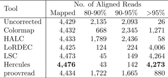
Table 3.2: Correction accuracy given high breadth of coverage (> 90%) in CH17-227A2.
Tool No. of Aligned Reads Mapped 80-90% 90-95% >95% Uncorrected 4,429 2,135 2,093 26 Colormap 4,432 668 2,345 1,271 HALC 4,433 1,789 2,436 58 LoRDEC 4,425 124 224 4,006 LSC 4,473 45 149 4,264 Hercules 4,476 43 142 4,273 proovread 4,434 1,722 1,665 880
The input included 9,449 PacBio reads which at least 90% of their length were covered by short reads. We report the accuracy as the alignment identity as calculated by the BLASR [57] aligner. Mapped column refers to the number of any reads aligned to the Sanger-assembled reference for this clone, where the other columns show the number of alignments within respective identity brackets.
3.2.3
Correction accuracy
After correction, we align the corrected reads to the corresponding ground truth using BLASR [57] with the noSplitSubreads option, which forces entire read to align, if possi-ble. Then, we simply calculate the accuracy of a read as reported by BLASR as alignment identity. We report the number of reads that align to the gold standard, and the align-ment accuracy in four different accuracy brackets. We observe that the number of confident alignments were the highest in both BAC clones and the human brain transcriptome for the reads corrected by Hercules (Table 3.1). Furthermore, for CH17-157L1, Hercules returned the largest number of corrected reads with the highest (>95%) accuracy. In contrast, the LoRDEC had slightly more reads with the highest (>95%) accuracy for CH17-227A2 com-pared to Hercules. We further investigated the reasons for lower Hercules performance for this clone, and we found that only ∼10% of the reads had > 90% short reads breadth cover-age. For such reads with better coverage, Hercules’s performance surpassed that of LoRDEC and all other correction tools (Table 3.2). See Section 3.3 for a discussion on the challenges of comparing accuracy of error correction tools.