Sasaki uzayında bir legendre eğrisi çevresindeki boru yüzeyi

* Corresponding Author

Received: 28 October 2018 Accepted: 01 June 2019

Tubular Surface Around a Legendre Curve in Sasaki Space Abdullah YILDIRIM

Harran University, Faculty of Arts and Sciences, Department of Mathematics, Şanlıurfa, Türkiye abdullahyildirim@harran.edu.tr , ORCID Address: http://orcid.org/0000-0002-6579-3799

Abstract

In this study, we described tubular surface around a Legendre curve in Riemannian Sasaki space with respected to Frenet frame. And than we give some definitions about special curve lying on this surface.

Keywords: Canal surfaces, Tubular surfaces, Connections, Geodesics, Sasaki

spaces, Legendre curve.

Sasaki Uzayında Bir Legendre Eğrisi Çevresindeki Boru Yüzeyi Özet

Bu çalışmada, Riemannian Sasaki uzayındaki Legendre eğrisi etrafındaki tübüler yüzeyini Frenet çatısına göre tanımladık. Bu yüzeyde yatan özel eğriler hakkında bazı tanımlar verdik.

Anahtar Kelimeler: Kanal yüzeyler, Boru yüzeyler, Konneksiyonlar, Geodezikler, Sasaki uzaylar, Legendre eğrisi.

Adıyaman University Journal of Science

dergipark.org.tr/adyusci

ADYUSCI

9 (1) (2019) 134-148

135 1. Introduction

Recall definitions and results[1, 5, 7]. If the four-elements structure (M,,,) provide the following conditions, it is called an almost contact manifold and the three-elements structure (,,) is called almost contact structure.

. 2 1 ) ( 0                I

where M , ,  and  are 3 manifold,  (1,1) tensor , (1,0) tensor and )

1 , 0

( tensor, respectively. Let g be a Riemannian metric on M If . ), ( ) ( ) , ( ) , ( X Y g X Y X Y g    

the five-elements structure (M,,,,g) is called an almost contact metric manifold. Moreover, if ), , ( ) , (X Y d X Y g   

the five-elements structure (M,,,,g) is named contact metric manifold where 

d is (0,2) tensor. On the other hand if

0 ) , ( 2 ) , ]( , [ ) , ( ) 1 (        Y X d Y X Y X N

for X,Y(M) then the five-elements structure (M,,,,g) is named Sasakian manifold. Next if , ) ( ) , ( ) (_X Yg X Y  Y X

the five-elements structure (M,,,,g) is Sasakian manifold where  is Levi-Civita connection on M . The opposite of the last sentence is also true.

If the structure vector  is a Killing vector field with respect to g i.e. Lg 0, the five-elements structure (M,,,,g) is called a K -contact structure.

136

The contact subbundle D_m



XT_M(m):(X)0



of TM is called contact distribution. The 1-dimensional integral submanifold of a contact distribution is called a Legendre curve.

In contact geometry, it is useful to give the following proposition, lemma and two theorems, which related to this study.

Proposition 1.1 [1,2] Let (,,,g) be contact metric manifold . If  is a Killing vector, we have

1) X X,

2) The sectional curvature of any plane spanned by  is 1.

Lemma 1.2 [1,2] Let M be a Sasakian manifold with the five-elements

structure M, , , , g . We obtain

RXY  YX  XY,

RXY  YX  gX,Y  XY.

Moreover, RXX  for all unit vector fields X orthogonal to  .

Theorem 1.3 [1,2] If R_XY (Y)X(X)Y, then M is a Sasakian manifold, where  is a Killing vector.

Theorem 1.4 Let M be a Sasakian manifold with the five-elements structure

M,,,,g . The torsion of its Legendre curve which is not geodesic is equal to 1. Proof. Let  be an unite speed non geodesic Legendre curve on M

 : I  Dm  M s  s  1s, 2s, 3s . We know ( ) 0 .    and ( ) . . T s 

 The Frenet vector fields of  is obtained as the following way

137 . , , . .       _{  } B N T

On the other hand we have

TT  T, TT  N. #

Afterward we can calculate the directional derivative of NT and  as follows. TN  TT  TT TT  T    T  B and . N T T        Hence   1. #

After now, we will admit that a Legendre curve is non geodesic an unite speed Legendre curve on M Sasakian space.

2. Tubular Surface

Let us recall the definitions and the results of [3]. A canal surface is named as the envelope of a family of 1-parameter spheres. In other words, it is the envelope of a moving sphere with varying radius, defined by the trajectory with center (t) and a radius function r(t) . This moving sphere S(t) touches it at a characteristic circle

) (t

K . If the radius function r(t)r is a constant, then it is called a tubular or pipe surface. Let



T,N,B



be the Frenet vector fields of  , where T , N and B are

138

tangent, principal normal and binormal vectors to  , respectively. Since the canal surface K(t,) is the envelope of a family of one parameter spheres with the center  and radius function r , it is parametrized as

Figure 1. A section of the canal surface (Doğan 2011).

). ( ) ( ) ( ) ( ) ( sin ) ( ) ( ) ( ) ( ) ( cos ) ( ) ( ) ( ) ( ) ( ) , ( 2 2 2 2 t B t t r t t r t N t t r t t r t t t r t r t t K                         

This surface is called the canal surface around the curve  . Clearly, N(t) and B(t) are spanning the plane that contains the characteristic circle. If the spine curve (s) has an arclenght parametrization



(s) 1



, then the canal surface is reparametrized as ). ( ) ( 1 ) ( sin ) ( ) ( 1 ) ( cos ) ( ) ( ) ( ) ( ) , ( 2 2 s B s r s r s N s r s r s T s r s r s s K             

139

For the constant radius case r(s)r , the canal surface is called a tubular (pipe) surface and in this case the equation takes the form



cos ( ) sin ( )



, ) ( ) , (s s r N s B s L       (1) where 0 2 .

After this, it will be admited that the tubular surface around of a Legendre curve is the tubular surface.

3. The Tubular Surface's Fundamental Forms

Let  (s): I E3 be Legendre curve. A parametrization L(s,) of the tubular surface has given in (1). The partial derivatives of L with respect to the

surface parameters s and  can be expressed in terms of Frenet vector fields of  as

























                     L T r L B r N r T r L B N r L L T r L B N r L s ss s                    sin , sin cos 1 sin cos sin cos , cos 1 , cos sin 2

We can also choose a unit normal vector field U of L as , sin cos N B L L L L U s s     _{ }   

where we know that



1 cos



2. 2 2 2    EG F r r L L_s      (2)

The first fundamental form I of L is defined as 2 2 2Fdxdy Gdy Edx I    where

140





. , , , , cos 1 , 2 2 2 r L L G r L L F r r L L E s s s                

On the other hand, the second fundamental form II of L is defined as

2 2 2fdxdy gdy edx II    in which





. , , , , cos 1 cos , r L U g r L U f r r L U e s ss                  

When on any surface EGF20 , it is regular surface.

Lemma 3.1 L

 

s, is a regular tube, iff cos 1,  0 and  0 .

Proof. It can easily be proved by using equation (2).

Theorem 3.2 Gaussian and the mean curvatures of a regular surface L , are

 

s t



 



  cos 1 cos 2 2 r r F EG f eg K       and





            Kr r F EG gE fF eG H 1 2 1 2 2 2 respectively.

4. Some Special Parameter Curves in The Tubular Surface

Theorem 4.1 [4,6,8] Let the curve  lie on a surface. If  is an asymptotic curve, then the acceleration vector is orthogonal to the normal vector of the surface. That is, U,  e0.

141

Theorem 4.2 Let L(s,) be tubular surface around focal curve of (s) . (1) If the L_s curves are asymptotic, then  r2cos(1cos) and cos 0 (2) The L curves are asymptotic.

Proof. For the s parameter curves we obtain the first coefficient e of second fundamental form as

) cos 1 ( cos ,  2    U L r e ss

showing that if the Ls curves is geodesic, then cos (1 cos )

2     r  . Because of , 0 

 cos 0. Similarly, for the t parameter curves we obtain the third coefficient g of second fundamental form as

0 ,  

U L r

g _

which implies that they can not be asymptotic.

Theorem 4.3 [5] Let the curve  lie on a surface. If  is a geodesic curve, then the acceleration vector  and the normal vector U of the surface are linearly dependent. That is, U  0.

Theorem 4.4 Let L(s,) be a tubular surface around a focal curve of (s), then

(1)The L_s curves cannot be geodesic (2) The L_ curves are geodesic curves.

Proof. For the s parameter curves, we have



















1 cos



. sin cos 1 sin sin cos 1 sin cos 2 B r N r T r L U _ss                        

142



















1 cos



0 sin , 0 cos 1 sin sin , 0 cos 1 sin cos 2                        r r r (3)

since the vectors {T,N,B} are linearly independent. However, since L(s,) is a regular surface, equation (3) can not be zero, namely r2sin



1cos



0 . Therefore

0

 L_ss

U which shows that Ls curves can not be geodesics. On the other hand,

since 0    L U rU U _

the  parameter curves L are geodesics. Converse is also true.

5. 3-dimensional Sasakian-Heisenberg Spaces

Let (x,y,z) be the standard coordinates on R and consider the 1-form 3



dzydx



 2 1  . We put z   2

 and consider the endomorphism of  defined by the matrix            0 0 0 0 1 0 1 0 y

with respect to the standard basis of R . Here 3 

 

 1 and 2I . Hence



,,



is an almost contact structure on R Next, we consider the metric tensor 3.





. 4 1 2 2 2 1    dx dx g

Its matrix representation with respect the standard basis is

             1 0 1 0 0 1 4 1 2 y y y y

143

Using the matrices of the metric g and of the endomorphism, we obtain

  

,



,

 X g X and d



X,Y

 

g X,Y



.

After some computations we obtain the connection coeffcients





. 2 1 , , 2 1 , 2 2 3 12 2 11 2 13 1 23 3 23 1 12 y y y                  

The vector fields

                        z e y e z y x e₁ 2 , ₂ 2 , ₃ 2 form an orthonormal basis with respect to g and e₁e_2,e₂ e_1,e₃ 0. Using the last equations we obtain . , , , 2 1 1 2 1 2 1 2 2 1 e e e e e e e e e e                     and



_x



Y g



X,Y





 

Y X.

Under the circumstances



_R3,,,.g



is a Sasakian manifold. If dual basis of orthonormal basis



e1,e2,e3



is





      _{    } ydx dz dy dx 2 1 , 2 , 2 3 2 1     .

Corollary 5.1 According to the metric g if 

 

s (₁(s),₂(s),₃(s)) is an unite speed Legendre curve in R 3,

 

1

 

. . 3 . y s s   

144

     

 

 

 

  . , , ) ( ₃ . 2 . 1 . 3 . 2 . 1 . . s z s y s x s s s s s         _                     

According to the orthonormal basis



e1,e2,e3



its shape is

 

 

_{ }

_{ }

. 2 1 2 2 ) ( _{1 3} . 3 . 2 2 . 1 1 . . e y s s e s e s s       _       

Because  is an Legendre curve in R 3, ( ) 0

.        s   namely

 

1

 

0 . 3 .   s y s  

where y is a coordinate fonction.

Example 5.1 Given the curve 

  

s  2sins,2coss,2cosssins2s



.  is an unite speed Legendre curve according to the metric g in R as Figure 2 shown 3

Figure 2. The Legendre curve 

Its velocity vector is

. sin cos ) ( _{1 2} . se se s    See that ( ) 0. .        s 

 Immediately we can obtain the Frenet vector



T,N,B



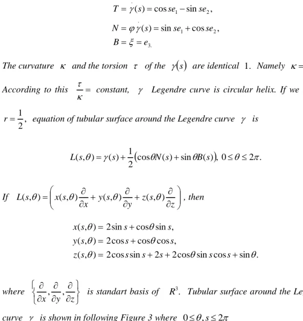
of  curve as follows

145 . 3 2 1 . 2 1 . , cos sin ) ( , sin cos ) ( e B se se s N se se s T            

The curvature  and the torsion  of the 

 

s are identical .1 Namely   1 . According to this 

 

constant,  Legendre curve is circular helix. If we choose

, 2 1



r equation of tubular surface around the Legendre curve  is



cos ( ) sin ( )



, 0 2 . 2 1 ) ( ) , (s   s  N s  B s    L If _               z s z y s y x s x s L( ,) ( ,) ( ,) ( ,) , then . sin cos sin cos 2 2 sin cos 2 ) , ( , cos cos cos 2 ) , ( , sin cos sin 2 ) , (                s s s s s s z s s s y s s s x where             z y x, , is standart basis of . 3

R Tubular surface around the Legendre curve  is shown in following Figure 3 where 0,s2

146

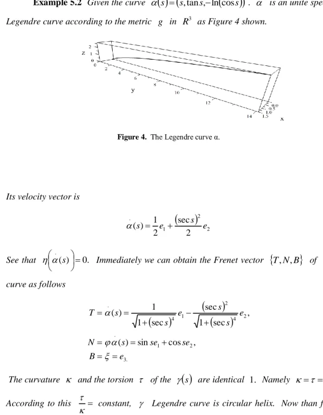
Example 5.2 Given the curve 

 

s 



s,tans,ln



coss





.  is an unite speed Legendre curve according to the metric g in R as Figure 4 shown. 3

Figure 4. The Legendre curve α.

Its velocity vector is





2 2 1 . 2 sec 2 1 ) (s  e  s e  See that ( ) 0. .        s 

 Immediately we can obtain the Frenet vector



T,N,B



of  curve as follows













. 3 2 1 . 2 4 2 1 4 . , cos sin ) ( , sec 1 sec sec 1 1 ) ( e B se se s N e s s e s s T              

The curvature  and the torsion  of the 

 

s are identical .1 Namely   1. According to this 

 

constant,  Legendre curve is circular helix. Now than for

, 1



r equation of tubular surface around  Legendre curve is



cos ( ) sin ( )



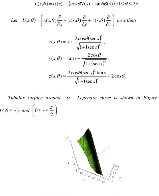
,0 2 . 2 1 ) ( ) , (s  s  N s  B s    L

147



cos ( ) sin ( )



, 0 2 . 1 ) ( ) , (s   s  N s  B s   L Let _               z s z y s y x s x s L( ,) ( ,) ( ,) ( ,) now than



















sec



2cos . 1 tan sec cos 2 ) , ( , sec 1 cos 2 tan ) , ( , sec 1 sec cos 2 ) , ( 4 2 4 4 2                 s s s s z s s s y s s s s x

Tubular surface around  Legendre curve is shown in Figure 5 where



0



and . 2 0       _{ } s

Figure 5. Tubular surface around Legendre curve α

References

[1] Belkhelfa, M., Hrca, E., Rosca, R. and Verstraelen, L., On Legendre Curves In

Remannan And Lorentzan Sasak Spaces, Soochow Journal Of Mathematcs, 28(1), 81–

91, 2002.

[2] Blair, D. E., Riemannian Geometry of Contact and Symplectik Manifolds, Boston, 2001.

148

[3] Doğan, F. and Yaylı, Y., On the curvatures of tubular surface with Bishop

frame, Commun. Fac. Sci. Univ. Ank. Series A1, 60(1), 59–69, 2011

[4] Hacısalihoğlu, H. H., Diferensiyel Geometri II, Hacısalihoğlu Yayınları, 2000. [5] Hacısalihoğlu, H. H. and Yıldırım, A., On BCV-Sasakian Manifold, International Mathematical Forum, 6(34), 1669–1684, 2011.

[6] Oprea, J., Differential Geometry and Its Applications, Prentice-Hall Inc., 1997. [7] Yıldırım, A., Tubular surface around a Legendre curve In BCV spaces, New Trends in Mathematical Sciences, 4(2), 61–71, 2016.

[8] Yıldırım, A., Tubular Surfaces Around a Tmelike Focal Curve In Mnkowsk 3-

Space, International Electronic Journal of Pure and Applied Mathematics, 10(2), 103–