Robust adaptive synchronization of dynamic networks with varying time delay coupling using varible structure control

Proceedings of the ASME 2014 Dynamic Systems and Control Conference DSCC2014 October 22-24, 2014, San Antonio, TX, USA

DSCC2014-6264

ROBUST ADAPTIVE SYNCHRONIZATION OF DYNAMIC NETWORKS WITH

VARYING TIME DELAY COUPLING USING VARIBLE STRUCTURE CONTROL

Vesna M. Ojleska

School FEIT, SS Cyril & Methodius University Institute of Automation & Systems Engineering

Karpos 2, MK-1000, Skopje, R. Macedonia

vojleska@feit.ukim.edu.mk

Dilek (Bilgin) Tükel

Department of Control&Automation Engineering Dogus University, Acibadem, TR-34722

Istanbul, Turkey

dtukel@dogus.edu.tr

Georgi M. Dimirovski

Department of Control&Automation Engineering Dogus University, Acibadem,Istanbul,Turkey School FEIT, SS Cyril & Methodius University Institute of Automation & Systems Engineering

Karpos 2, MK-1000, Skopje, R. Macedonia

gdimirovski@dogus.edu.tr

ABSTRACT

The synchronization problem for a class of delayed complex dynamical networks via employing variable structure control has been explored and a solution proposed. The synchronization controller guarantees the state of the dynamical network is globally asymptotically synchronized to arbitrary state. The switching surface has been designed via the left eigenvector function of the system, and assures the synchronization sliding mode possesses stability. The hitting condition and the adaptive law for estimating the unknown network parameters have been used for designing the controller hence the network state hits the switching manifold in finite time. Two illustrative examples along with the respective simulation results are given, which employ the designed variable structure controllers.

INTRODUCTION

Network structures have been subject of research for considerable time in mathematical systems and control science as well as in physics. Furthermore, it has been observed for some time that complex dynamic networks exist in all fields of science and humanities as well as in the nowadays networked technical and non-technical systems, such formations of moving objects and individuals or societal groups. Thus the latter

systems have been studied extensively over the past couple of decades. As it is well-known, traditional networks are mathematically represented by a graph, e.g. a pair G=

{ }

P,E in which P represents a set of N nodes (or vertices)

N P P

P₁, ₂,L, _{and E is a set of links (or arcs or edges)} N

L L

L1, 2,L, each of which connects two elements in P . The well known chains, grids, lattices and fully connected graphs have been formulated to represent the so-called completely regular networks.

(a) (b)

Fig. 1: A random graph network (a), and a small-world network (b) [7]

In due course of developments, the theory of random graphs (Figure 1-a) was first introduced by Paul Erdos and

Alfred Rényi [1], who discovered the probabilistic methods were often useful to tackle problems in graph theory. In recognition to their work, now these are known as ER random graph models. The ER random graph models have served as idealized coupling architectures for gene networks and the spread of infectious diseases for a long time, and recently for studying the spread of computer viruses too.

In recent studies, Watts and Strogatz [2] introduced the so-called small-world networks (Figure 1-b), or so-so-called WS networks, in order to describe the transition from a regular network to a random network [3], [7]. Subsequently, in their studies [4-6], Barabasi and Albert have argued that the scale-free nature (Fig. 2) of real-world networks is rooted in two general mechanisms: growth and preferential attachment respectively. It thus gives rise to dynamical nodes in networks and not solely static ones. In the real world at large, many real systems such as biological, technological and social systems can be described by various models of complex networks [8], [9]. One of the interesting and rather significant phenomena in complex dynamical networks [10] is the synchronization of all dynamical nodes as well as the appearance of chaotic modes.

Fig. 2: A scale-free network [7]

In this paper, a class of general complex dynamical network models with coupling delays is explored with regard to the controlled synchronization by applying the variable structure control theory. The synchronization properties of these models with matched conditions uncertainty and unmatched conditions uncertainty by using of the variable structure control VSC are investigated.

Via Lyapunov functional methodology and by formulation of an adequate proper adaptive law, we derive synchronization conditions for both cases. The next section presents a selected survey, a continuous-time dynamical network model with coupling time-delays and some preliminaries. In subsequent section, the switching surface for the SVC is constructed by using the left eigenvector function method.

The stabilities of the network synchronized states in both cases, with known bounds and with unknown bounds on

nonlinear terms, are investigated in the two sections, respectively, thereafter. Then, the obtained results and computer simulations for two of benchmark examples are given. Concluding section and references follow thereafter.

FORMULATION OF DYNAMIC NETWORK MODEL AND APPLICATION OF THE VSC

The synchronization in networks of coupled chaotic systems has received a great deal of attention during the last decade or so, e.g. see [10]-[18] for instance. In their work [10], Wang and Chen have established a uniform dynamical network model for such studies; also they explored its synchronization and control. Although, the model of Wang and Chen reflects the complexity from the network structure, still it is a fairly simple uniform dynamical network. A new model and chaos synchronization of general complex dynamical networks was also explored by Hu and Chen in [11], and by Lu and co-authors in [12]. Further, Wang and Chen [13] explored the synchronization problem in small-world dynamical networks, and similarly Barhona and Pecore studied the synchronization in heir small world systems in [14]. In [15], Wang and Chen investigated the synchronization in scale-free networks with regard to robustness and fragility. Subsequently, X. Li and Chen discussed synchronization and de-synchronization of complex dynamical networks from an engineering point of view in [16].

More recently, in works [17]-[21], the complex dynamical networks with time-delays have received particular attention more attentions because its presence is frequently a source of instability. For, time-delays commonly, or even unavoidably, exist in various network-like systems due to some inherent mechanism and/or the finite propagation speed of information carrying signals. Z. Li and Chen proposed in [17] a linear state feedback controller design to realize the synchronization for the networks with coupling delays. Similarly, C. Li and Chen proposed a solution in the case with coupling delays in work [18]. Further, P. Li and co-authors explored in [19] one way of global synchronization in delayed networks, and Z. Li and co-authors in [20] solved the same with regard to desired orbit. It should be noted controlled synchronization in complex dynamical networks with either nonlinear delays or with coupling delays in [18]-[21] was studied via the methodology of Lyapunov stability analysis. In parallel, also the design of robust decentralized control for large-scale systems with time-varying or uncertain delays has been revisited via several approaches and feasible designs derived in [22]-[25]. These studies too have been carried out via Lyapunov stability analysis and synthesis. The approach via variable structure control (VSC) is to be noted for their efficiency in dealing with all sorts of time-delay and uncertainty phenomena in dynamical systems.

We consider a complex dynamical network consisting of N identical nodes (

n

dimensional dynamical systems) with time varying delay coupling

, )) ( ( ) , ( 1

∑

= − + + + = N j i i ij j ij i i i Ax f x t A x t t Bu x& τ N i=1,2,L, ₍₁₎ Where: xi=(xi1,xi2,L,xin)T∈Rn, represents the state vector of the i-th node; f(xi,t):

n n

R R

R × → are smooth nonlinear vector function; τ_ij(t) is bounded time varying delay and differentiable too satisfying 0≤τ_ij(t)≤τ_ij <∞, whereτ_ijis positive scalar; and

∑

= − N j ij j ijx t t A 1 )) (

( τ represent the uncertain interconnections with time delay. Furthermore, A∈Rn×n,

m n i R

B ∈ × are constant system matrices of appropriate dimensions, and u_i∈Rm represents the control input. When the network achieves synchronization, namely, the state

N x x

x = =L= 2

1 , as t−>∞, the coupling control terms

should vanish: ( ()) 0 1 = + −

∑

= i i N j ij j ijx t t Bu

A τ . This ensures that

any solution x_i(t) of a single isolate node is also a solution of the synchronized coupled network.

Let s(t) be a solution of the isolate node of the network, which is assumed to exist and is unique, satisfying:

(

s t

)

f As

s&= + , . (2) In here s(t) can be an equilibrium point, a nontrivial periodic orbit, or even a chaotic orbit. The objective of control here is to find some smooth controllers ui∈Rm such that the solution of systems (1) asymptotically synchronize with the solution of (2), in the sense that

0 ) ( ) ( lim − = →∞ xi t st x , i 1,2, ,N L = (3)

Let it be defined ei=xi(t)−s. Then subtracting (2) from (1) yields the error dynamical system

i i N j ij j ij i i i Ae f x s A x t t Bu e = + +

∑

− + =1 )) ( ( ) , ( ~ τ & ₍₄₎ where ) , ( ) , ( ) , ( ~ t s f t x f s x f _i = _i − .

For deriving the proofs, given in sequel, certain convenient assumptions are given next.

Assumption 1: The matrix pair

(

A, B_i

)

is controllable. Assumption 2: Each input matrix B is of full rank. _i Assumption 3: The nonlinear function f satisfying

) ( ) ( ) , ( ) , (x t f x t x t x t f _i − _j ≤µ_{i i} − _j (5) where µi>0 are constants, i,j=1,2,L,N.

Assumption 4: Suppose the interconnection matrix satisfy matching condition as follow:

ij i ij BH

A = (6) Assumption 5: The time delay terms in system (4) satisfy

) ( )) ( (t t x max t xj −τij ≤ j (7) where ) ( max ) ( max t x t x_j = _j .

Therefore equation (4) can be rewritten as follows:

∑

= − + + + = N j i i ij j ij i i i i Ae f x s BH x t t Bu e 1 )) ( ( ) , ( ~ τ & ₍₈₎

CONSTRUCTING THE SWITCHING SURFACE FOR APPLYING VARIABLE STRUCTURE CONTROL

The composite sliding surface of system (8) is defined by letting the composite sliding vector σ(e)in the state space be zero. This is to say that

( )

e

[

σ₁T(e₁), σ₂T(e₂), σT_N(e_N)

]

σ = L ₍₉₎ where

( )

i = i i=0 ie Ce σ ,i=1 L, ,N (10) are called the local sliding surface and e=

[

e1T, L, eTN

]

∈RN, while C are _i m×n constant matrices to be determined in due course.

In order to construct the controller sought, the following two relevant lemmas from the literature are needed as well.

Lemma 1 [24]. Suppose β and b₁,b₂,L,b_{N be arbitrary} vectors, then

∑

∑

= = ≤ + N i i T i T N i T _{b a a b b} a 1 1 1 ) ( 2 β β (11)

where β >0 is a positive constant.

Lemma 2[24]. Suppose matrix _

     = 22 12 12 11 D D D D D _T and its inverse matrix _      = 22 12 12 11 Π Π Π Π Π T         − = ₋ − − Ψ Ψ Π Π 1 11 12 1 13 12 11 11 1 D D D D D _T (12) where Ψ =(D₁₃−D₁₂TD₁₁−1D₁₂)−1 and 1 12 1 13 12 11 11 ( ) − − − = T D D D D

Further, let the isolate subsystem as follows i i i i Ae Bu e& = + (13) be selected. Because

(

A, B_i

)

is controllable, there exists matrix K_i∈Rm×n that can make the matrix A~_i=A+B_iK_i be stable. And B is full rank matrix, we can assume _{i }

     = i i B B ~0 , m m i R

B~ ∈ × . When the controller u_i=K_ie_i+v_i is substituted in to (13), the equation is transformed to

2 12 1 11 1 ~ ~ i i i i i A e A e e& = + ₍₁₄₎ i i i i i i i A e A e Bv e&₂= ~_{21 1}+ ~_{22 2} + ~ ₍₁₅₎ Assume the stability eigenvalues of Ai

~ are m in i im i λ µ µ −

λ1,L, , 1,L, , and then define:

          = −m in i i µ µ Λ O 1 1 ,           = im i i λ λ Λ O 1 2 (16) The corresponding eigenvectors constitute the eigenvector

matrix as _      2 1 2 1 i i i i V V G G

. The eigenvector matrix is the inverse through the pole placement, so that the following equation holds             =               2 1 2 1 2 1 22 21 12 11 2 1 2 1 0 0 ~ ~ ~ ~ i i i i i i i i i i i i i i V V G G A A A A V V G G Λ Λ (17)             =               − − 2 1 1 2 1 2 1 1 2 1 2 1 22 21 12 11 0 0 ~ ~ ~ ~ i i i i i i i i i i i i i i V V G G V V G G A A A A Λ Λ (18)       =       − 2 1 2 1 1 2 1 2 1 i i i i i i i i V V G G η η ξ ξ (19)             =               2 1 2 1 2 1 2 1 2 1 22 21 12 11 0 0 ~ ~ ~ ~ i i i i i i i i i i i i i i A A A A Λ Λ η η ξ ξ η η ξ ξ (20) Therefore 1 1 1 12 1 11 ~ ~ i i i i i i A A ξ + η =ξ Λ (21)

From the above, we know that _      2 1 2 1 i i i i η η ξ ξ is the right eigenvector matrix of _       22 21 12 11 ~ ~ ~ ~ i i i i A A A A . If we select

[

i1 i2

]

i V V C = (22) when the system trajectory hit the sliding mode, i.e.σ_i=C_ie_i=V_i1e_i1+V_i2e_i2, then 1 1 1 2 2 i i i i V V e e =− − (23) Substitution of (23) into (14) yields the sliding mode equation

1 1 1 2 12 11 1 ) ~ ~ ( _{i i i i i} i A A V V e e& = − − ₍₂₄₎ Because V_i2∈Rm×m and (G_i1−G_i2V_i−₂1V_i1) are inverse, and due to Lemma 2, it follows

1 1 1 2 1 i i i i V V ξ η ₌₋ − ₍₂₅₎

Also upon substitution of (25) into (21) yields 1 1 1 1 1 2 12 11 ) ~ ~ (A_i −A_i V_i−V_i ξ_i =ξ_iΛ_i (26) From the above we can know the eigenvalues of the sliding mode equation of system (13) represent the desired n−m stable eigenvalues. It is obvious that the sliding mode equation (14) is stable. From the above analysis, Ci is the left eigenvector of Ai

~

with desired m stable eigenvalues, then i

i i

iA C

C ~ =Λ₂ (27)

For the error complex system (4), because the coupling term is satisfying the matching condition, the sliding mode equation of system (4) is still satisfying equation (24), which has the desired eigenvalues. If the nonlinear and the coupling terms do not satisfy the matching condition, the system (4) can be written as follows ) , ( ~ ~ ~ 1 2 12 1 11 1 A e A e f x s e&i = i i + i i + i i (28) i i N j ij j ij i i i i i i i i v B t t x H B s x f e A e A e ~ )) ( ( ~ ~ ) , ( ~ ~ ~ 1 2 2 22 1 21 2 + − + + + =

∑

= τ & (29)

When σ_i=0, then ei2=−Vi2−1Vi1ei1, so the above sliding mode equation of system (28) is ) , ( ~ 1 1 1 Ae f x s e&i = i i + i i (30) where 1 ₁ 2 12 11 ~ ~ i i i i i A A V V

The first novel result is the synchronization condition for the complex network with unmatched uncertainty that is given according the next theorem.

Theorem 1. If the nonlinear term ~f(xi,s) is unmatched, then the decentralized sliding mode of the interconnected system (30) is asymptotically stable, if and only if the inequality

) (

1 i i i i

kµ <−β λ +β (31) holds true, where k1>0 is constant, and

{

,

}

0

max 1 <

= i im

i λ λ

λ L _.

Proof: Let

V

be a candidate Lyapunov function for the dynamic system (30),

∑

= = N i i T ie e V 1 1 1 & ₍₃₂₎

Taking the derivative of

V

along the trajectory of system (30) yields

[

]

∑

= + = N i i i i T i Ae f x s e V 1 1 1 1 ( , ) ~ 2 & ₍₃₃₎

Due to Assumption 3, there exist positive constant

k

₁ that makes ~f_i1(x_i,s) ≤k₁µ_ie_i1 . Thus 2 1 1 2 1 2 1 1 i i i i i i i e e k e V µ β β λ + + ≤ & 2 1 1 1 i i i i i k e       + + = µ β β λ (34)

due to Lemma 1. And then becauseλi<0, if i i i

i _β kµ λ β + 1 <−

1

it follows V&<0 at once.

DESIGNING THE SYNCHRONIZATION CONDITION: KNOWN BOUNDS ON NONLINEAR TERMS

Although we have a set of stable sliding surfaces, unless the initial states and all system dynamics are always ensured to stay on the surface for all time, a set of decentralized sliding controllers is required, such that the global robust stability of the surface is assured. Traditionally, the hitting condition for small-scale system is 0 ) ( ) (tTσ t < σ & ₍₃₅₎

where σ(t)=0is the sliding surface of some small-scale systems. Since the existence of interconnections and the lack of global information, equation (35) is not easily satisfied for the interconnected system. Hence, we require a global hitting condition of the sliding surface

0 ) ( ) ( ) ( 1 <

∑

= N i i i i i i T i e e e σ σ σ & (36) If

∑

= = N i i V 1

σ , the condition is readily derived from the stability theory of Lyapunov .

Theorem 2: The motion of the system (4) asymptotically converges to the composite sliding surface σ(e)=0, if and only if the following condition

i i i i i i i i i Ke CB R e u σ σ 1 ) ( − − = , (37) where

∑

= + + = N j j ij i i i i i C CB H x t R 1 max() ε µ

and

ε

>

0

is constant, is satisfied.

Proof: From (4) and (10), the sliding dynamics can be written as i i i C &e & ₌ σ

∑

= − + + + = N j i i i j ij i i i i i iAe C f x s C BH x t CBu C 1 ) ( ) , ( ~ τ

∑

= − + + + − = N j j ij i i i i i i i i i i i i i t x H B C s x f C u B C e K B C 1 2 ) ( ) , ( ~ τ σ Λ (38)

Upon substitution of (37) into (38), the (38) can be written down as

∑

= − + + − = N j j ij i i i i i i i i i R e C f x s C BH x t 1 ~ 12 . ) ( ) , ( τ σ σ σ Λ σ (39) Then construct Lyapunov function as

∑

= = N i i i d V 1 σ (40)

and obtain the time derivative of (40) as

∑

= = N i i i T i i d V 1 σ σ σ & & ₍₄₁₎

Substitution of (37) and (39) into (41) yields

[ ]

∑

= = N i i T i i V d V 1 σ Σ σ & _(42-a)

[ ]

VΣ =         − − + +

∑

= N j i i i i ij j ij i i i i i i Cf x s CBH x t R e 1 2 ( , ) ( ) ~ σ σ τ σ Λ (42-b)

Because of

λ

_i

=

max{

λ

_i1

,

L

,

λ

_im

}

<

0

and Assumption 2, it follows that

∑

∑

= =           − − + + ≤N i N j i i i ij j ij i i i i i i i i i i e R d t x H B C d e C d d V 1 1 ) ( τ µ σ λ &

[

]

∑ ∑ ∑ = = =         + − − − − = N i i N j ij j ij i i i i i i N i i i i e R t x H B C e C d d 1 1 1 ) ( τ µ σ λ . 0 ) ( ) ( 1 1 max 1 1 1 < − − − + =

∑ ∑

∑ ∑

∑

= = = = = N i N j j ij i i i N i N j ij j ij i i i N i i i i t x H B C d t x H B C d d ε τ σ λ (43)

Thus, on the grounds of the designed controller and according to Theorem 2, the motion of the system (4) asymptotically converges to the composite sliding surface.

DESIGNING THE SYNCHRONIZATION CONDITION: UNKNOWN BOUNDS ON NONLINEAR TERMS

In practical terms, there exist ~f(x_i,s) ≤µ_i e_i , where µ_i represents unknown parameters. In this section, we will design robust adaptive controller with unknown parameters. In order to derive the proof, conveniently, first another two assumptions are presented.

Assumption 6: Let rank

(

~f, B_i

)

=rank

( )

B_i . Assumption 7: Let _      = i i B B 2 0 , whereB_2i∈Rm×m is an nonsingular matrix.

When the transformation u_i=K_ie_i+v_i is selected, then the sliding mode equation becomes

1 1 1 2 12 11 1 ) ~ ~ ( _{i i i i i} i A A V V e e& = − − _{. (44)} It is fairly easy to prove the asymptotic stability of the sliding mode trajectory by the constructing switching function. Therefore the main task here is to design a robust controller that guarantees the system trajectory shall reach the sliding surface from an arbitrary initial state.

Theorem 3 Let Assumption 4 and Assumption 5 hold true. Then with

i i i

=

C

e

µ

&ˆ

, µ~i=µˆi−µi, (45-a) the following robust adaptive controller

− = i i i Ke u           + + −

∑

= − _N j i i j ij i i i i i i i x H B C e C B C 1 max 1 sgn ˆ ) ( σ ε µ , (45-a)

where

µ

ˆ

_i is the estimate of the unknown parameter, and µi, 0

> i

ε are constants, uniformly, asymptotically stabilize the system (4) in the large.

Proof: Consider the Lyapunov function as follows

∑

∑

= = + = N i i N i i V 1 2 1 ~ 2 1 _µ σ (46)

The time derivative of (46) is as follows:

∑

∑

= = + = N i i i N i i i i i T i e e V 1 1 ˆ ~ ) ( ) ( _µµ σ σ σ & & &

∑

∑

∑

= = = +                   − + + + − = N i i i N i _N j ij j ij i i i i i i i i i i i i i i T i t x H B C s x f C u B C e K B C 1 1 1 2 ˆ ~ ) ( ) , ( ~ µ µ τ σ Λ σ σ & . ˆ ~ ) ( 1 1 1 1 i N i i i N i i i N i N j i i i ij j ij i i i i i i i i i i i u B C t x H B C e C e K B C ε σ λ µ µ τ µ σ λ − ≤ +             + − + + − ≤

∑

∑

∑

∑

= = = = & (47)

Because of λ_i<0, ε_i>0, apparently (47) is negative. Thus, the system (4) can be stabilized by means of the controller (45-a, b) , which is designed according to Theorem 3.

ILLUSTRATIVE EXAMPLES AND COMPUTER SIMULATIONS

The chaotic Chua circuit is assumed in the nodes of the complex dynamical network. A singular Chua circuit is described by the piecewise-linear system

)) ( ( x y f x p

x&= − + − _,&_y=_x−_y+_{z, z}&=−_qy where ) 1 1 )( ( 2 1 ) (x =m0x+ m1−m0 x+ −x− f

with constants m₀<0 and m₁<0, p=10, q=14.87, 68 . 0 , 27 . 1 ₁ 0=− m =− m . Let it be set 1

,

2

,

3

x

=

x x

=

y x

=

z

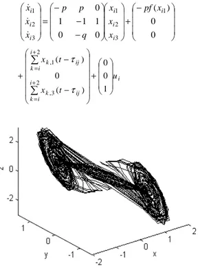
. Then this Chua circuit can also be represented as follows: )) ( ( _{1 2 1} 1 p x x f x x& = − + − _, 3 2 1 2 x x x x& = − + _, 2 3 qx x& = _.

The corresponding complex network with coupling time-delay is represented by          − +                     − − − =           0 0 ) ( 0 0 1 1 1 0 1 3 2 1 3 2 1 i i i i i i i pf x x x x q p p x x x & & & i i i k ij k i i k ij k u t x t x           +               − − + ∑ ∑ + = + = 1 0 0 ) ( 0 ) ( 2 3 , 2 1 , τ τ

Fig. 3: Trajectories of chaotic chua circuit in its 3D state space.

In order to simulate it conveniently, it has been assumed 02

. 0 < ij

τ . On the grounds of Theorem 1, the synchronization error trajectory of chaotic Chua circuit can be computer simulated to give the results on synchronization shown in Fig. 4. These results show the synchronization has been enforced rather efficiently by synchronization employing the proposed variable structure control design.

Fig. 4: Synchronization errors ei1 of chaotic Chua circuit.

The Duffing forced-oscillation system is used as nodes in a dynamical network. A singular Duffing forced-oscillation system is described as

y

x&= _{, y&=−0.1y−x}3_+12cost

Let it be defined x₁=x, x₂=y. Then the Duffing forced-oscillation system can also be expressed as follows:

2 1 x x& = _{, x 0.1x x}3 _12cost 1 2 2=− − + &

Its phase portrait is depicted in the next figure.

Fig. 5: Trajectory of Duffing forced-oscillation system in its 2D state (phase) space.

The corresponding network is described by       + − +             − =       t x x x x x i i i i i cos 12 0 1 . 0 0 1 0 3 1 2 1 2 1 & & i i i k ij k i i k ij k u t x t x       +             − − +

∑

∑

+ = + = 1 0 ) ( ) ( 2 1 , 2 1 , τ τ

Fig. 6: The synchronization errors of the Duffing forced-oscillation system.

By using making use of the controller in Theorem 3, the synchronization error trajectories of Duffing forced-oscillation system has been simulated and the error signals are depicted in Fig. 6. These simulation results show that the network synchronization by the designed variable structure controller is enforced rather efficiently.

CONCLUSION

The synchronization problem in coupled complex dynamic delay network has been explored. Both systems with known bound and with unknown bound on nonlinear terms have been successfully taken into consideration. Stability solutions to synchronization are proposed that employ variable structure control theory along with constructive design of the sliding surfaces and the switching. The switching surface has been designed via the left eigenvector function of the system, which can assure the synchronization sliding mode possesses stability. The hitting condition and the adaptive law for estimating the unknown network parameter have been used for designing the controller, which can assure the network state hitting the switching manifold in finite time.

The two benchmark examples, based on employing chaotic Chua circuit and on Duffin’s oscillator at the nodes, have been used for illustrating the performance via synchronization error trajectories. The respective computer simulations demonstrated both efficient network synchronization as well as quality transient performance.

ACKNOWLEDGMENT

This research was supported in part by the joint Turkish-Russian scientific research project (grant TUBITAK-RFBR-113E595) in Aerospace Sciences, the joint Turkish-Russian scientific research project (grant TUBITAK-RFBR-113E595) in Aerospace Sciences and by Funds for Science of the School FEEIT at SS Cyril and Methodius of Skopje and of Dogus University of Istanbul.

REFERENCES

[1] Erdös, P., Rényi, A., 1960, “On the evolution of random graphs,” Publications Math. Inst. Hung. Acad. Sci., vol. 5, pp. 17-61, 1960.

[2] Watts, D. J. , Strogatz, S. H. 1998, “Collective dynamics of small-world networks,” Nature, vol. 393, pp. 440–442, 19.

[3] Watts, D. J., 1999, Small-Worlds: The Dynamics of

Networks between Order and Randomness. Princeton University Press, Princeton, NJ.

[4] Barabasi, A. L., Albert, R., 1999, “Emergence of scaling in

random networks,” Science, vol. 286, pp. 509–512.

[5] Barabasi, A. L., Albert, R. , Jeong, H., 1999, “Mean-field theory for scale-free random networks,” Physca A, vol.

272, pp. 173–187.

[6] Liu,T., Dimirovski, G.M., Zhao,J., 2008, “Exponential synchronization of complex delayed dynamical networks with general topology,” Physica A – Statistical Mechanics and Its Applications, vol. 387, is. 2–3, pp. 643–652.

[7] Strogatz, S. H., 2001, “Exploring complex networks,” Nature, vol. 410, pp. 268–276.

[8] Yang, X.S., 2001, “Chaos in small-world networks,”

Physics Review E, vol. 63, pp. 46-206.

[9] Wang, X. F., 2002, “Complex networks: topology,

dynamics and synchronization,” Int. J. Bifurcation and Chaos, vol. 2, no. 5, pp. 885–916.

[10]Wang, X. F., Chen, G., 2003, “Complex networks: small-world, scale-free, and beyond,” IEEE Circuits and Systems Magazine, vol. 3, no. 1, pp. 6–20.

[11]Hu, J.L.,Chen, G., 2003, “New general complex dynamical network models and their controlled synchronization criteria,” A preprint (private communication).

[12]Lu,J., Yu, X., Chen,G., 2004, “Chaos synchronization of general complex networks dynamical, Physica A, vol. 334, pp. 281-302.

[13]Wang, X. F., Chen, G., 2002, “Synchronization in small-world dynamical networks,” Int. J. Bifurcation and Chaos, vol. 12, pp. 187–192.

[14]Wang, X. F., Chen, G. , 2002, “Synchronization in scale-free dynamical networks: robustness and fragility, IEEE Trans. on Circuits & Systems, vol. 49, no. 1, pp. 54–62.

[15]Barahona, M., Pecora, L. M., 2002, “Synchronization in small world systems,” Physics Review Letters, vol. 5, pp. 54-101.

[16]Zhong,W.S., Dimirovski, G.M, Zhao, J., 2009, “Decentralized synchronization of an uncertain complex dynamical network,” Journal of Control Theory and

Applications, vol. 7, no. 3, pp. 225-230.

[17]Li Z., Chen, G., 2004, “Robust adaptive synchronization of uncertain dynamical networks,” Physics Letters A , vol. 324, pp. 166–178.

[18]Li, C., Chen, G., 2004, “Synchronization in general complex dynamical networks with coupling delays,” Physica A, vol. 343, pp. 263 – 278.

[19]Li, P., Yi, Z., Zhang, L., 2006, Global synchronization of a class of delayed complex networks, Chaos, Solitons and Fractals, vol. 30, pp. 903-908.

[20]Zhou, J., Chen, T.P., “Synchronization in general complex delayed dynamical networks,” IEEE Trans. on Circuits &Systems, vol. 53, pp. 733-744, 2006.

[21] Li, Z., Feng G., Hill, D., “Controlling complex dynamical networks with coupling delays to a desired orbit,” Physics Letters A, vol. 351, pp. 42-46, 2006.

[22]Wang, L., Jing Y., Kong, Z., Dimirovski,G.M, “Adaptive exponential synchronization of uncertain dynamical networks with delay couplings,” Neuro-Quantology: An International Journal of Neurology and Quantum Physics, vol. 6, no. 4, pp. 397-404, 2008.

[23]Chou, C.H., Cheng, C-C., “A decentralized reference adaptive variable structure controller for large-scale time-varying delay systems,” IEEE Trans. on Automatic Control, vol. 48, pp. 1213-1217, 2003.

[24]Lee, J. L. , Wang, W-J. , “Robust decentralized stabilization via sliding mode control, Control Theory and Advanced Technology, vol. 10, no. 2, pp. 622-731, 2003.

[25]Shyu,K.K., Liua, W.J., Hsu, K.C. “Design of large-scale time-delayed systems with dead-zone input via variable structure control,” Automatica, vol. 41, 1239-1246, 2005.