MODELING, ANALYSIS AND SIMULATION OF SIMPLE
ONE MACHINE–TWO PRODUCT SYSTEM USING
PETRI NETS
BASİT BİR MAKİNE–İKİ ÜRÜN SİSTEMİNİN PETRİ AĞLARI KULLANILARAK MODELLENMESİ, ANALİZİ VE SİMULASYONU
Özgür ARMANERİ
Dokuz Eylül University, Department of Industrial Engineering
ABSTRACT : As in many engineering fields, the design of manufacturing systems
can be carried out using models. Petri nets have been used extensively to model and analyze manufacturing systems. Petri Nets, as graphical and mathematical tools, provide a uniform environment for modeling, format analysis and design of discrete event systems. The modeling, simulation and analysis of simple one machine-two product systems using Petri nets will be presented in this paper. Behavioral and structural properties of the Petri net model will be considered in details. Then, the Petri net model of one machine-two product system will be simulated using a simulation program.
Keywords : Petri Nets, Petri Net modeling, one machine-two product systems. ÖZET : Çoğu mühendislik alanlarında olduğu gibi imalat sistemlerinin tasarımı, modeller kullanılarak başarılabilir. Petri ağları imalat sistemlerinin modellenmesi ve analizinde yaygın olarak kullanılmaktadır. Petri ağları, şekilsel ve matematiksel araçlar olarak kesikli olay sistemlerinin modellenmesi, biçimsel analizi ve tasarımı için düzenli, iyi bir ortam sağlar. Bu makalede, basit bir makine-iki ürün sistemlerinin Petri ağları kullanılarak modellenmesi, simülasyonu ve analizi sunulacaktır. Petri Ağı modelinin davranışsal ve yapısal özellikleri ayrıntılı olarak incelenecektir. Daha sonra bir makine-iki ürün sisteminin Petri ağı modelinin bir simülasyon programı kullanılarak simülasyonu gerçekleştirilecektir.
Anahtar Kelimeler : Petri ağları, Petri Ağı modelleme, bir makine-iki ürün sistemler.
1. Introduction
In view of complex nature of modern industrial systems, the design and operation of these systems require modeling and analysis in order to select the optimal design alternative, and operational policy. Petri nets, as graphical and mathematical tools, provide a uniform environment for modeling, formal analysis, and design of discrete event systems. One of the major advantages of using Petri net models is that the same model is used for the analysis of behavioral properties and performance evaluation, as well as for systematic construction of discrete-event simulators and controllers. Petri net were named after Carl A. Petri who created in 1962 a net-like mathematical tool for the study of communication with automata. Petri net can be used to model properties such as process synchronization, asynchronous events, concurrent operations, and conflicts or resources sharing.
It is highly desirable for researchers, system analysts and production engineers to have a unified mathematical model for modeling, analysis, simulation planning and control of manufacturing systems. Petri nets as graphical tools provide a powerful communication medium between the user, typically requirements engineer and the customer. Complex requirements specifications, instead of using ambiguous textual descriptions of mathematical notations difficult to understand by the customer, can be represented graphically using Petri nets. This combined with the existence of computer tools allowing for interactive graphical simulation of Petri nets, puts in hands of the development engineers a powerful tool assisting in the development process of complex systems (Zurawski and Zhou, 1994, p.567).
The aim of this paper is to show how to use Petri nets in order to model, analyze and simulate one machine-two product manufacturing systems. The manufacturing system considered in this paper can be thought as one of the module of complex industrial systems. Paper is organized as follows. The literature review is presented in Section 2. The underlying system definition is discussed in Section 3. Behavioral and structural properties of the Petri net model are presented in Section 4 and Section 5, respectively. Section 6 introduces the simulation of the constructed Petri net model. Conclusions and recommendations are given in the last section.
2. Literature Review
There are many varieties of Petri nets from simple net (black and white Petri nets), which are conceptually simple and straightforward to analyze, to more complex nets such as colored nets, timed nets and stochastic nets (Murata, 1989, pp.541-580). Petri nets have been used extensively to model and analyze manufacturing systems. In this area, Petri nets were used to represent; simple production lines with buffers, machine shops, automotive production systems, flexible manufacturing systems, automated assembly lines, resource-sharing systems, and just in time and kanban
manufacturing systems. In this paper how to model and analysis one machine-two
product systems will be investigated. There are several studies for the analysis and modeling of these kinds of systems.
For example, in the paper, which is written by Alpan and Jafari in 1997, two products and a shared resource systems was discussed. In that paper, they present a method, they call “Relative Temporal Analysis”, to analyze the dynamics of this system. It is possible to find the resource utilization sequence, the waiting time period for each product and identify possible conflicts through this technique. Based on that technique they also build control charts that can be used for control purposes such as obtaining “optimal” conflict resolution schemes.
In the paper that is written by Narahari, Hemachandra and Gaur in 1995, the performance of a machine that processes several classes of jobs with significant setup times and with priority scheduling is examined. The machine serves three classes of jobs – class 1, class 2 and class 3 – class 3 jobs have non-preemptive priority over jobs of class 1 and class 2. The results show that the throughput and cycle time of class 1 and class 2 jobs are affected quite dramatically by the arrival of class 3 jobs. Several other studies in the literature have explored performance and scheduling issues connected with a shared resource machine. See, for example, the books by Viswanadham and Narahari (1992), Buzacott and Shantikumar (1993) and
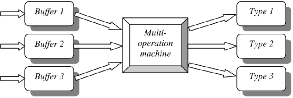
Gershwin (1994). In this article there is a single multi-operation machine producing 3 types of products.
Figure 1 gives a schematic. Let the nonpriority jobs be called type 1 and type 2 jobs, whereas the priority jobs are called type 3 jobs. The machine switches production among these products by giving non-preemptive priority to type 3 jobs and takes up type 1 or type 2 jobs only when there are no type 3 jobs waiting for production; it takes up type 1 jobs when there are no type 2 jobs and vice versa. (In the case of both type 1 and 2 waiting it chooses type 1 or type 2 with probability 0.5 each). In contrast, while serving type 1 or type 2 jobs (with no type 3 jobs waiting), it follows an exhaustive policy, i.e., once setup for a particular type, say type 1, processing is done on all type 1 parts until no more type 1 parts are waiting in the buffer. Finally, the processing of all jobs is non-preemptive.
Figure 1. A Multi-Product Manufacturing Facility
In the design and analysis of the manufacturing systems, the validation of their models is often addressed via simulation; this allows analyzing both the transient and the steady state behavior of the modeled system. In this paper, firstly an example related to one machine-two product system will be given and the Petri net model of this system will be constructed. Then this Petri net model will be simulated in order to understand the model working easily. For simulating the model, a computer simulation program should be used. Lopez and Mellado (1995) who wrote the paper that is named “Simulation of Timed Petri Net Models”, considered one of the simulation program in their paper. This paper deals with simulation of timed Petri net based models; they present an efficient algorithm for the execution of generalized timed transition Petri nets (TTPN). They gave an algorithm for TTPN simulation.
3. System Definition
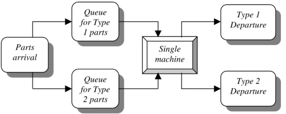
In the considered manufacturing system, two different part types arrive to a workstation consisting of a single machine. The time between part arrivals is exponentially distributed with a mean of five minutes. The distribution of arriving parts is 80% Type 1 and 20% Type 2. The part types are maintained in separate queues in front of the machine. Type 1 parts have priority over Type 2 parts, and hence the machine only processes a type 2 part if no type 1 parts are available. However, once processing of a Type 2 part begins, it is not interrupted by an arriving Type 1 part. The processing time for each part type is normally distributed
Multi-operation machine Buffer 1 Buffer 2 Buffer 3 Type 3 Type 2 Type 1
with a mean of four minutes and a standard deviation of two minutes. The schematic diagram of manufacturing system is shown in Figure 2.
Figure 2. A Single Multi-Operation Machine and Two-Product System
There are two separate queues and only one multi operation machine in the system. In general, machines are multi-operation, which means that they can perform several types of operation. In Figure 3, it is given the model of a machine, which is able to perform two operations on two types of product denoted by Type 1 and Type 2.
t1 Type 1 Type 2 t2
Figure 3. A Petri Net Model of a Multi-Operation Machine
A queue can be represented in Petri net models as seen in Figure 4.
Figure 4. Petri Net Model of a Queue
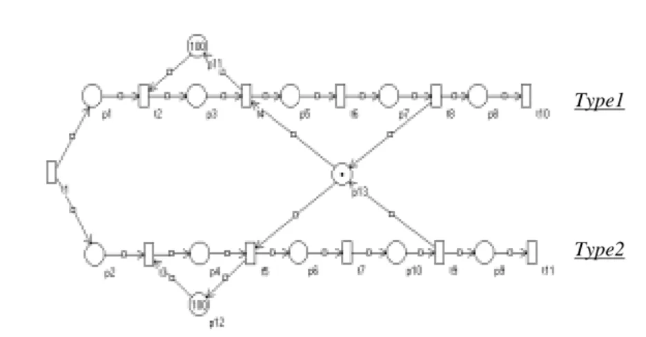
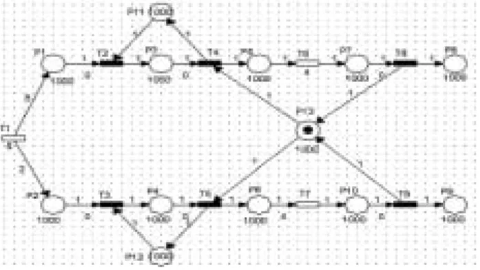
As a consequence, the Petri net model of this one multi-operation machine and two product manufacturing system can be constructed as in Figure 5.
Single machine Parts arrival Queue for Type 1 parts Queue for Type 2 parts Type 1 Departure Type 2 Departure
Figure 5. A Petri Net Model of One Machine-Two Product System
To understand the system better, it is necessary to give some explanation. Firstly, we
can say that the transition t1 represents parts arrival. So when transition t1 is fired,
new parts (type 1 or 2) enter the system. After part arrival, the part types are
maintained in separate queues in front of the machine. t2, p3, t4, p11, t2 and t3, p4, t5,
p12, t3 construct event graphs. These event graphs represent the separate queues of
type 1 and type 2. The weights of arcs between (t1,p1) and (t1,p2) are equal to 8 and
2, respectively.
In order to obtain the queue length and to specify the situation of queue, it is assumed that both of the separate queues’ capacities are 1000 units of parts in simulation program.
There is a conflict in this Petri Net model. If both transition t4 and t5 can be fired,
then it must be specified which transition would fire. Type 1 parts have priority over Type 2 parts, and hence the machine only processes a type 2 part if no type 1 parts
are available. So if both transition t4 and t5 can be fired, firstly transition t4 will fire.
4. Behavioral Properties of the Petri Net Model
The behavioral properties discussed in this section are boundedness, reversibility, liveness and home state. Descriptions of other properties can be found in Murata (1989). The p-invariants and t-invariants of the Petri Net model have to be found in order to specify the behavioral properties of the net. A vector Z with n columns and one row and with non-negative integer elements is a p-invariant if; Z * U = 0, where
U is the incidence matrix of the Petri net and n the number places in the Petri net.
Then, a vector W with one row and q columns (q is the number of transitions of the Petri net under consideration) and with non-negative integer elements is a t-invariant
if; U * Wt = 0. The incidence matrix, U, is shown below;
Type1
0 0 1 1 0 0 1 1 0 0 0 0 0 0 0 0 0 1 0 1 0 0 0 0 0 0 0 0 0 1 0 1 0 0 0 1 0 1 0 0 0 0 0 0 1 0 1 0 0 0 0 0 0 0 0 0 1 0 1 0 0 0 0 0 0 0 0 0 0 1 0 1 0 0 0 0 0 0 0 0 0 1 0 1 0 0 0 0 0 0 0 0 0 1 0 1 0 0 0 0 0 0 0 0 0 1 0 1 0 0 0 0 0 0 0 0 0 1 0 1 0 0 0 0 0 0 0 0 0 1 0 1 0 0 0 0 0 0 0 0 0 1 1 13 12 11 10 9 8 7 6 5 4 3 2 1 11 10 9 8 7 6 5 4 3 2 1 − − − − − − − − − − − − − − = p p p p p p p p p p p p p t t t t t t t t t t t U
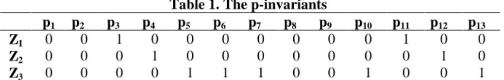
The p-invariants calculated by using DNANET computer program are shown in Table 1.
Table 1. The p-invariants
p1 p2 p3 p4 p5 p6 p7 p8 p9 p10 p11 p12 p13
Z1 0 0 1 0 0 0 0 0 0 0 1 0 0
Z2 0 0 0 1 0 0 0 0 0 0 0 1 0
Z3 0 0 0 0 1 1 1 0 0 1 0 0 1
This Petri net model includes a source transition. There are 13 places in the net and nine of them are covered by invariants. However 4 of them are not covered by
p-invariants. So these places, named as “p1, p2, p8 and p9”, are not bounded. As known,
if one of the places of a Petri net is unbounded, a Petri net is unbounded. So the underlying Petri net is unbounded.
The three levels of coverability tree of the net are shown in Figure 6.
t1
t2 t3
t2 t4 t2 t5
Figure 6. The Three Levels of Coverability Tree of the Net
0,0,0,0,0,0,0, 0,0,0,100,100,1 w,w,0,0,0,0,0, 0,0,0,100,100,1 w,w,0,1,0,0,0, 0,0,0,100,99,1 w,w,1,0,0,0,0, 0,0,0,99,100,1 w,w,0,0,1,0,0, 0,0,0,100,100,0 w,w,2,0,0,0,0,0, 0,0,98,100,1 w,w,0,2,0,0,0, 0,0,0,100,98,1 w,w,0,0,0,1,0, 0,0,0,100,100,1
As seen in Figure 6, the coverability tree of the Petri net contains the symbol “w”. So it is confirmed that this Petri net is unbounded.
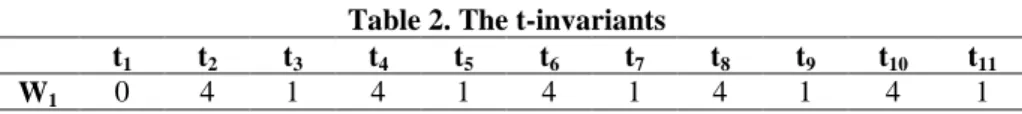
The t-invariant calculated by using DNANET is shown in Table 2.
Table 2. The t-invariants
t1 t2 t3 t4 t5 t6 t7 t8 t9 t10 t11
W1 0 4 1 4 1 4 1 4 1 4 1
If the same element in all the t-invariants of the Petri net model of a manufacturing system is equal to zero, then it is claimed that it is impossible to come back to the initial marking after firing a sequence of transitions which contains the transition corresponding to this element. From a manufacturing point of view, this means that it will be impossible to come back to the initial state if we perform the operation represented by the transition corresponding to the null element of the t-invariants.
Here, there is only one t-invariant and the value of t1 is equal to zero. In addition,
this transition is a source transition. So this Petri Net is not reversible.
A Petri net is said to be live if all its transitions are live. A transition t of a Petri net is said to be live if it can be fired from any marking M reachable from the initial
marking M0. In this Petri net, there is not markings M reachable from the initial
marking M0 is a deadlock. So this system is deadlock-free. Thus, all transitions can
be fired. Therefore this Petri Net model is live.
A marking Ma of a Petri net with initial marking M0 is a home state if it is reachable
from any marking reached from M0. However, it could not be specified if this Petri
Net model has home states. Because the reachability tree of the Petri net is very complex.
5. Structural Properties of the Petri Net Model
Structural properties depend only on the structure of the Petri net, and not on the initial marking and the firing policy. These properties are thus of great importance when designing manufacturing systems, since they depend only on the layout and not on the way the system will be managed, which is not known at the design level. (Proth and Xie, 1996, p.83)
A Petri net is said to be structurally live if there exists an initial marking M0 such
that Petri net is live. In other words, a Petri net that is live is structurally live. Therefore, it can be said that this Petri net model is structurally live.
A Petri net is said to be structurally bounded if the marked Petri net is bounded for
any initial marking M0. There is a source transition in the model. So the total
number of tokens in the system can be increased. Because of that reason this Petri net model is not structurally bounded.
A Petri net is said to be consistent if there exists an initial marking M0 and a
sequence σ of firable transitions which contains at least once each transition and
which, when fired, leads again to M0. As mentioned, this Petri net model is not
reversible and it is impossible to come back to the initial marking again. So this Petri net model is not consistent.
A Petri net is said to repetitive if there exists an initial marking M0 and a firable
sequence σ in which each transition appears an unlimited number of times. In other words, a Petri net that is structurally live is repetitive. This Petri net is structurally live, so it is repetitive.
6. Model Simulation
The constructed Petri net model of the system can be simulated by using a program. There are several simulation programs concerned with the Petri net simulation. Some of them are DNANET, WinTTPN, HPSim and Visual Object Net 20. However the conflict situation and the normal distribution of the transition firing times cannot be shown in these programs. On the other hand, in this Petri net model, the conflict situation is important, and the processing time for each part type is normally distributed. So, it should be made some assumptions for simulating of the Petri Net model. These assumptions are as follows;
(i) Type 1 parts haven’t priority over Type 2 parts.
(ii) The processing time for each part type is exponential distributed with a mean of four minutes.
(iii) The last two transitions, named as t10 and t11, were dropped for representing
how many parts were produced in 480 minutes simulation time. So the
number of parts in p8 and p9 places gives us how many parts were produced
in that time.
(iv) Place capacities effect the simulation of the model. If any place capacity is not enough, then simulation does not go on. So all places capacities are taken as 1000 parts.
(v) It is assumed that the queues capacities are unlimited. So, the queues capacities are taken as a large value, for example 1000 parts.
HPSim simulation program is used for simulating the Petri net model. The model constructed using HPSim is shown in Figure 7. Notice that the last two transitions,
named as t10 and t11, were dropped.
Figure 7. The Petri Net Model Constructed Using HPSim
After simulating the Petri net model for 480 minutes, the situation of the model in 480. minute is shown in Figure 8.
Figure 8. The Situation of the Petri Net Model in 480. Minute
The obtained statistics at the end of 480 minutes are as follows;
Table 3. The Statistics at the End of 480 Minutes Produced parts
in 480 minutes
The average flow time for each parts
The length of each queue at the end of 480 minutes
Type 1 62 7.7419 minutes 769 parts
Type 2 67 7.1642 minutes 141 parts
After simulating the Petri net model, the flow times of the first and second part types are determined as 7.74 and 7.16 minutes, respectively. In addition, the length of each part queue (separate queues) at the end of 480 minutes was recorded. If the number of waiting parts in separate queues at the end of 480 minute is considered, it is seen that the number of waiting Type 1 parts in a queue is absolutely greater then the number of waiting Type 2 parts in a queue. However, if Type 1 parts are available in the system, then the machine should process these parts. For that reason, while there were too many Type 1 parts waiting in the queue, Type 2 parts should not be produced. However, as specified before, none of the simulation program on hand allows showing conflict situation and priority. Hence, the assumption (i) was satisfied. So, there are many Type 2 parts produced more than expected value and the number of Type 1 parts waiting in the queue was very high.
7. Conclusions and Recommendations
Petri nets are powerful tools in modeling the operating modes of machines, transportation systems, tools, buffers, etc. In this paper, Petri nets, their behavioral and structural properties and the related analysis methods have been introduced. Then, it has been shown how to use Petri nets to model, analyze and simulate one machine-two product manufacturing systems.
Simulating the Petri net model with simulation programs suitable for the structure of the manufacturing system is necessary for determining the accuracy of the constructed model and understanding the model working. However, the simulation program that permits to show conflicts and priority situations could not be obtained. So, some assumptions have been made. Then, it was shown that the constructed Petri net model represents the real manufacturing system with respect to these assumptions.
The use of Petri nets may lead to models of excessive size. A solution to this problem is to use a modular approach which consists in decomposing manufacturing systems into modules, in modeling the modules, in verifying that the module models have all the desired qualitative properties, in simplifying the module models while preserving their qualitative properties, and in integrating the simplified module models in a way that preserves the desired qualitative properties (Proth and Xie, 1996, p.189). The manufacturing system considered in this paper can be thought as one of the module of a complex system. Therefore, the next step of the study is to integrate the module models in a way that preserves the qualitative properties of the modules.
References
ALPAN, G., JAFARI, M.A. (1997) Dynamic analysis of timed Petri Nets : a case of two products and a shared resource. IEEE Trans. Robot. Automation, vol 13, no. 3, June.
BUZACOTT, J.A., SHANTIKUMAR, J.G. (1993) Stochastic models of
manufacturing systems. New Jersey, Prentice-Hall.
GERSHWIN, S.B., (1994) Manufacturing systems engineering. New Jersey, Prentice-Hall.
LOPEZ, E., MELLADO, J. (1995) Simulation of timed Petri Net Models. IEEE Inc.
Con. Of Syst. Man.Cyb., vol. 3, no.2.
MURATA, T. (1989) Petri Nets : properties, analysis and applications. Proceedings
of the IEEE, vol. 77, no. 4, April.
NARAHARI, Y., HEMACHANDRA, N., GAUR, M.S. (1995) The Analysis of multiclass manufacturing systems with priority scheduling. Computers Ops. Res., vol. 24, No.5, February.
PROTH, J.M., XIE, X. (1996) Petri Nets: a tool for design and management of
manufacturing systems. Baffins Lane, Chichester, John Wiley&Sons.
VISWANADHAM, N., NARAHARI, Y. (1992) Performance modeling of
automated manufacturing systems. New Jersy, Prentice-Hall.
ZURAWSKI, R., ZHOU, M. (1994) Petri Nets and industrial applications : a tutorial. IEEE Transactions on Industrial Electronic, vol. 41, no. 6, December.