Control of subsonic cavity flows by neural networks-analytical models and experimental validation

Control of Subsonic Cavity Flows by Neural Networks –

Analytical Models and Experimental Validation

M. Ö. Efe1_{, M. Debiasi}2_{, P. Yan}3_{, H. Özbay}3,∗ _{and M. Samimy}2,§

Collaborative Center for Control Science The Ohio State University, Columbus, Ohio

1_{Dept. of Electrical & Electronics Eng., TOBB University of Economics and Technology}

Sögütözü, 06530, Ankara, Turkey

2_{Dept. of Mechanical Eng., The Ohio State University} 3_{Dept. of Electrical and Computer Eng., The Ohio State University}

∗_{Dept. of Electrical & Electronics Eng., Bilkent University, 06800, Ankara, Turkey} §_{Corresponding author, E-mail: samimy.1@osu.edu}

Flow control is attracting an increasing attention of researchers from a wide spectrum of specialties because of its interdisciplinary nature and the associated challenges. One of the main goals of The Collaborative Center of Control Science at The Ohio State University is to bring together researchers from different disciplines to advance the science and technology of flow control. This paper approaches the control of subsonic cavity flow, a study case we have selected, from a computational intelligence point of view, and offers a solution that displays an interconnected neural architecture. The structures of identification and control, together with the experimental implementation are discussed. The model and the controller have very simple structural configurations indicating that a significant saving on computation is possible. Experimental testing of a neural emulator and of a directly-synthesized neurocontroller indicates that the emulator can accurately reproduce a reference signal measured in the cavity floor under different operating conditions. Based on preliminary results, the neurocontroller appears to be marginally effective and produces spectral peak reductions analogous to those previously observed by the authors using linear-control techniques. The current research will continue to improve the capability of the neural emulator and of the neurocontroller.

I. Introduction

This study presents the results obtained up to date in the analytical development and the experimental validation of neural-network based techniques for cavity flow control. This work is part of a larger multidisciplinary effort in developing fundamental understanding and implementation of feedback control techniques applied to fluid flows.

Influencing the behavior of a flow field is a core issue as it could yield significant increase of the efficiency and performance of fluidic systems (Cattafesta 1997). However, the tools of classical control systems theory are not directly applicable to the fluid flows with spatial continuity and non-linear behavior, which pose formidable modeling challenges due to the infinite dimensionality and complexity of the governing Navier-Stokes equations.

Neural networks (NNs), on the other hand, are well known for their powerful nonlinear mapping capabilities. The computational flexibility and the diversity of algorithms allowing the designer to tune for a given map make neurocomputing a good alternative for flow modeling and control (Haykin 1994; Jang et al. 1997). With reference to

American Institute of Aeronautics and Astronautics 1 43rd AIAA Aerospace Sciences Meeting and Exhibit

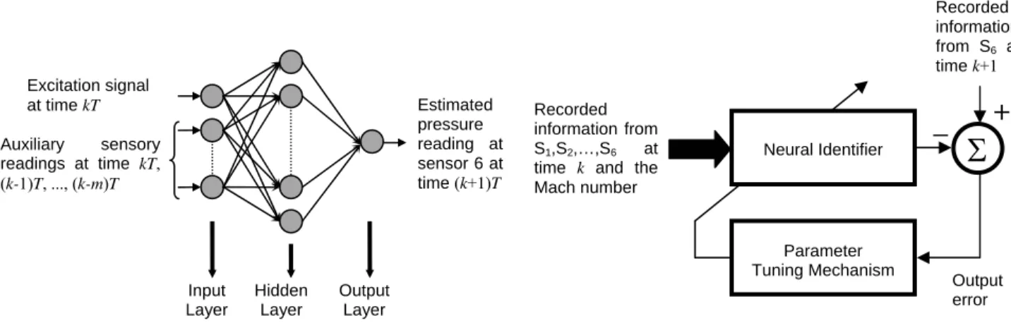
the specific study case of this work, Debiasi and Samimy (2004a), a small wind tunnel with a cavity recessed in the test section floor has been used, Fig. 1, and it has been demonstrated that given some history of the inputs (excitation or control signal) and outputs (pressure readings from some particular locations of the cavity), a NN based feedforward model can be developed such that the model emulates the input-output behavior of the process under investigation (Efe et al. 2004). The input in this context is the excitation signal (S1) to the compression driver

actuator, Fig. 1, and the output is the signal at of the dynamic pressure transducer number 6 (S6) in the middle of the

cavity floor, Fig. 2. The motivating factor for using such an approach is that the technique exploited here is data oriented, i.e. the experimental data can directly be utilized to obtain a describing input-output model, compactly containing the effect of process as well as the actuators, sensors and even the contribution of experimental disturbances. A number of architectural alternatives are available to derive such a model. The structure of a Feedforward Neural Network (FNN) with input-output definitions for our goal is illustrated in Fig. 3. Similarly, when the parameter adjustment issues enter into the picture, there are well-founded optimization techniques for this purpose, e.g. the Error Backpropagation (EBP) (Rumelhart et al. 1986), Gauss-Newton, conjugate gradient method, Levenberg-Marquardt technique (LM) or derivative-free approaches (Jang et al. 1997). In this paper, we utilize the Levenberg-Marquardt technique as it converges significantly faster than those mentioned above, (Hagan and Menhaj 1994).

Some work has been carried out in the past decade to explore the use of NN techniques in flow control with various degrees of success. Among these are efforts exclusively focused on the numerical simulation of the flow model and of the corresponding control. Jacobson and Reynolds (1993) conducted a numerical study on the control of wall shear layer in a boundary layer by using feed-forward NN as controllers, which showed skin friction reduction by about 8%. The study of active laminar flow control by Fan et al. (1993) showed that properly trained NN can establish complex nonlinear relationships between multiple inputs and outputs which are characteristic of an active flow control system. They also used experimental data but did not validate the control experimentally. Faller et al. (1994) obtained a NN model of a pitching airfoil based on experimental data. With limited training data the model predicted unsteady surface pressure topologies within 5% of the experimental data. Kawthar-Ali and Acharya (1996) conducted a similar study but obtained a more marginal performance improvement. The simulation of Lee et al. (1997) on the use of an adaptive controller based on NN to reduce drag in a turbulent channel flow predicted 20% drag reduction. Interestingly in this study a simpler control scheme was derived from NN that produced the same amount of drag reduction. An extended survey is presented in Kim (2003). Yuen and Bau (1998) used a NN-based approach to suppress chaotic convection in a thermal convection loop. The NN was connected in series with the plant and it utilized the back-propagation algorithm to compute the weights and biases of the neurons. Adaptive controller developed later by the same authors provided a better performance than this NN controller, (Yuen and Bau 1999). Finally, Giralt et al. (2000) used NN to model the nonlinear dynamics of the turbulent flow past a cylinder. The method was able to capture and identify the coherent and disordered motions in the flow.

In the next sections, we describe the experimental apparatus, the algorithm and the procedures used in this study to train the neural emulator and the neurocontroller followed by the results observed with experimental implementations of these techniques.

II. The Experimental Facility

In this study, the experimental facility described in detail in Debiasi and Samimy (2004a) is used, which consists of an optically accessible, blow-down type wind tunnel capable of continuous operation in the subsonic range. A shallow cavity with a depth D = 12.7 mm and length L = 50.8 mm and having length to depth aspect ratio L/D = 4 is recessed in the floor of the test section. For control the cavity shear-layer is forced by a 2-D synthetic-jet type actuator issuing from the end slot of a high-aspect-ratio converging nozzle embedded in the cavity leading edge and spanning the width of the cavity, Fig 1. Pressure fluctuations are measured by dynamic pressure transducers placed in different locations in the test section, Fig. 2. As visible in the same figure, windows enable visualization of the flow field inside the test section utilizing advanced laser-based techniques developed at the Gas Dynamics and Turbulence Laboratory (GDTL) of OSU. Flow imaging techniques are used to capture the instantaneous and phase-averaged features of the flow as described in Samimy et al. (2004).

Since the experimental facility enables us to acquire pointwise observations from the critical locations of the cavity, one could use this information for identification and control of the cavity flow. This is done using a dSPACE 1103 DSP board connected to a Dell Precision Workstation 650. This system acquires simultaneously at 50 kHz the pressure transducer signals through 16-bit input channels and manipulates them to produce the desired control signal from a 14-bit output channel. Each recording is band-pass filtered between 200 and 10,000 Hz to remove spurious

frequency components. The simultaneous time traces collected from these transducers have been used to train the NN with the characteristics described in Efe et al. (2004) and in Yan et al. (2004). It is critically important to emphasize that the data must be spectrally rich enough to capture cases that are likely to be encountered in real-time operation. Additional recordings of 262,144 samples per channel through a 16-bit resolution acquisition board (National Instruments PCI-6036E) are acquired at 200 kHz and used to derive SPL spectra as described in Debiasi et al. (2004b).

Debiasi and Samimy (2004a) observed that the cavity flow exhibits strong, single-mode resonance in the Mach number ranges 0.25-0.31 and 0.39-0.5, and multi-mode resonance in the Mach number range 0.32-0.38. In the same study, they also observed that the frequency of sinusoidal forcing with the synthetic jet-like actuator has a major impact on the cavity flow resonance whereas the effect of the amplitude is relatively minor and it affects the control authority only at higher Mach numbers. This prompted the development of a control that uses a logic-based feedback to search the forcing frequencies that reduce the cavity flow resonant peaks and then maintains the system in such conditions through an open-loop control. The technique performed well and allowed identification of optimal forcing frequencies (OpFF) for the reduction of resonant peaks in the Mach number range 0.25-0.50.

Some linear feedback controllers were also developed for subsonic cavity flows by the Collaborative Center of Control Science (Samimy et al. 2004, Yan et al. 2004, and Debiasi et al. 2004b) and the experimental results offered two important conclusions: (i) all the linear controllers derived from a linear plant model for a single dominant Rossiter mode (Rossiter 1964) were able to suppress the cavity oscillations at this mode, but they shifted the oscillations to another Rossiter frequency, which was not present explicitly in the unforced case; and (ii) adding a zero to the simplest of these controllers, the proportional controller, avoided this problem, provided that the location of the zero matches the newly excited Rossiter mode mentioned above. The real time implementations in dSPACE (Yan et al. 2004, Debiasi et al. 2004b) showed in particular that the parallel proportional (PP) controller with a time delay block outperforms the other linear controllers (classical PID controller, Smith predictor and H-Infinity controller) in terms of elimination of the main frequency of oscillation and robustness with respect to departure from the design flow conditions. The resonant peak reduction is comparable to that obtained with OpFF, but the method is more robust with respect to slight changes in flow parameters.

These simple yet effective control techniques represent a reference against which alternative control strategies could be compared, e.g. neurocontrollers or controllers that exhibit some degree of autonomy and intelligence.

III. Levenberg-Marquardt Algorithm for Training the Neural Network Structures

Development of a model emulating the behavior of the flow based on established approaches, e.g. by using the Navier-Stokes governing equations, is a challenging task. A good alternative for doing this is to utilize the NN structures as emulators (identifiers). Referring to Fig. 4, one sees that the relevant input pattern, S1…S6 up to time k,

the Mach number, and the desired pattern, S6, which is up to time k+1, are available from off-line recorded

measurements, and the parameters of the emulator are adjusted in such a way that a quadratic cost function based on the output error is minimized. Although the EBP technique is quite popular for NN training purposes, it is a first order method, i.e. it uses the first order partial derivatives of the cost function. On the other hand, LM technique utilizes the second order derivatives and therefore finds a better path towards the minimum of the cost function. Despite its computational burden stemming from the matrix inversion at each iteration, the training performance is superior to EBP, (Hagan and Menhaj 1994, Jang et al. 1997, Efe 1996). The analytical procedure for LM optimization scheme is summarized as follows.

The algorithm is an approximation to the Newton’s method, and both of them have been designed to solve the nonlinear least squares problem (Hagan and Menhaj 1994). Consider a NN having O outputs, and N adjustable parameters denoted by the vector ω. If there are P data points (measurements, or patterns) over which the interpolation is to be performed, a cost function qualifying the performance of the interpolation can be given as

( )

_{∑ ∑}

(

( )

)

p O

o dop xop

E ω _{1 1} ω 2 , (1)

where xop is the value at the oth output of the neural emulator in response to the pth pattern, and dop is the

corresponding target entry. It should be noted that in this study only the value at S6 is of interest and therefore O=1

and dop denotes the recorded sensory value at S6. The parameter update prescribed by Newton’s algorithm is given

as

( )

(

)

( )

where ωk refers to time step k and ωk+1 refers time step k+1. We should note that

( )

( ) ( ) ( )

Eω 2 ω T ω ω

2

ω = +

∇ and ∇_ωE

( )

( ) ( )

being the error vector and the Jacobian as given in (3) and (4) respectively.

[

]

In (3), it is seen that the error vector is computed for all outputs of the NN and all patterns. For example, eop

means the difference between the oth _{NN output and the corresponding o}th _{entry in a target vector, which is the}

desired vector in the pth _{training pattern.}

⎥ ⎥ ⎥ ⎥ ⎥ ⎥ ⎥ ⎥ ⎥ ⎥ ⎥ ⎥ ⎥ ⎥ ⎥ ⎥ ⎥ ⎥ ⎦ ⎤ ⎢ ⎢ ⎢ ⎢ ⎢ ⎢ ⎢ ⎢ ⎢ ⎢ ⎢ ⎢ ⎢ ⎢ ⎢ ⎢ ⎢ ⎢ ⎣ ⎡ ∂ ∂ ∂ ∂ ∂ ∂ ∂ ∂ ∂ ∂ ∂ ∂ ∂ ∂ ∂ ∂ ∂ ∂ ∂ ∂ ∂ ∂ ∂ ∂ ∂ ∂ ∂ ∂ ∂ ∂ ∂ ∂ ∂ ∂ ∂ ∂ = N OP OP OP N P P P N P P P N O O O N N e e e e e e e e e e e e e e e e e e J ω ) ω ( ω ) ω ( ω ) ω ( ω ) ω ( ω ) ω ( ω ) ω ( ω ) ω ( ω ) ω ( ω ) ω ( ω ) ω ( ω ) ω ( ω ) ω ( ω ) ω ( ω ) ω ( ω ) ω ( ω ) ω ( ω ) ω ( ω ) ω ( ) ω ( 2 1 2 2 2 1 2 1 2 1 1 1 1 2 1 1 1 21 2 21 1 21 11 2 11 1 11 L M M M L L M M M L M M M L L (4)

the Gauss-Newton algorithm can be formulated as

( ) ( )

(

)

( ) ( )

and the LM update can be constructed as

( ) ( )

(

)

( ) ( )

where µ > 0 is a user-defined scalar design parameter. Clearly, the Gauss-Newton method assumes that the entries of the matrix g(ωk) are negligibly small in magnitude, and the LM technique improves the rank deficiency problem of

the matrix J(ωk)TJ(ωk). It is important to note that for large values of µ Eqn. (6) becomes the standard Gauss-Newton

method, Eqn. (5), and for small values of µ, the tuning law becomes the standard EBP algorithm. Therefore, LM method is a good balance between EBP and Gauss-Newton algorithms.

IV. Training of the Emulator (Identifier)

In training the emulator, the NN is asked to realize the mapping from current state of the flow and external excitation to the next state of the flow. The state of the flow is described by the information acquired from the chosen sensors. Define the following variables:

S1 measures u1,k, the voltage to the actuator,

S2 measures u2,k, the pressure fluctuations just before the actuator exit (See Fig. 2),

S3 measures u3,k, the pressure fluctuation just after the actuator exit (i.e. at the receptivity region

at the cavity leading edge),

S4 measures u4,k, the pressure fluctuations in the freestream before the cavity,

S5 measures u5,k, the pressure fluctuations at the cavity trailing edge,

S6 measures dk, the pressure fluctuations at the center of the cavity floor.

With these definitions, a NN emulator will realize the series-parallel model

(

)

1 k k k n k k k m k k k p

k f d d d u u u u u u

x + = − − − − − − , (7)

where the optimization problem is to build the function f and the parameters m,n,…,p are the user-specified delay-depths on selected channels. In addition to these, xk is a prediction for dk. One should notice that the Mach number

could be an external input to the NN model. If such an approach succeeds, this would let us have a generalized NN emulator that can be used at different Mach numbers (i.e. different flow regimes). Towards this goal, sets of 100,000 samples for S1, S3, S5 and S6 were acquired simultaneously at 50 kHz as described in section II. We considered the

flow regimes at Mach numbers 0 (no flow), 0.25, 0.28, 0.30, 0.32 and 0.35, without forcing and with OpFF and white noise forcing.

In order to validate the modeling claim of the paper, the mechanism illustrated in Fig. 4 has been implemented with different simple feedforward NN structures. We found a structure having 8 inputs, 4 hyperbolic tangent hidden neurons and one linear output neuron to be particularly effective. The NN performs the following mapping

(

)

1 k k k k k k k

k f d d d d u u u

x + = − − − , (8)

and the training data is the white noise excited cases. Every experiment contributes 8,190 lines of data to the ultimate training data set containing the effect of relevant cases, and a total of 147,420 training pairs have been prepared. After 20 epochs of tuning with Levenberg-Marquardt algorithm, the convergence occurs as shown in Fig. 5.

The validation of the obtained NN model is shown in Figs. 6 and 7 for the unseen data. In these figures, dk and xk

denote the desired (already recorded) value and predicted value (by NN), respectively. The similarity of the desired and estimated signals in both time and frequency domains are encouraging for extending the approach for control purposes that is discussed next.

V. Training of the Neurocontroller

Based on to what has been reported in the neurocomputing and flow control literatures, a NN controller for the described flow system can explore the nature of the problem from two different viewpoints, assuming that the sensory information is sufficient to obtain an emulator and a controller. The first alternative is the direct synthesis of a controller, which is illustrated schematically in Fig. 8. The underlying philosophy is straightforward: sensors S3, S5

and S6 are chosen for illustrating the concept. The signal at u1,k, which is the control signal, causes a transition from

state [u3,k, u5,k, u6,k] to [u3,k+1, u5,k+1, u6,k+1]. When training the emulator, the NN is asked to realize the map NNE:[u1,k,

u3,k, u5,k, u6,k]→[u3,k+1, u5,k+1, u6,k+1], however, the directly synthesized controller should ask for the following map

NNC:[u3,k, u5,k, u6,k, u3,k+1, u5,k+1, u6,k+1]→[y1,k] ≈ [u1,k], i.e. given the state transition, what is the input signal leading to

that transition? Then, for a library of different transitions, the neural controller learns the relation between each state transition and the control signal leading to that particular transition. Not surprisingly, such a NN, if it exists, would function as a controller.

The second method is the indirect synthesis, which entails the use of an emulator. A pre-trained emulator is connected parallel to the flow system as shown in Fig. 9. The reason for using an emulator is that it is a feedforward model enabling the calculation of sensitivity derivatives needed in tuning the controller parameters. To be explicit, the partial derivatives of the output with respect to the inputs are needed in propagating the output error back through the emulator. The emulator parameters are not modified during this phase. When the error at the output of the controller is obtained, the controller tuning can be done. The controller training takes place on-line and as time progresses, the controller learns/improves how to fulfill the specified task. Typical disadvantages of using such a scheme are the computational burden, possible insufficiency of the emulator performance, and the difficulty in analyzing the closed loop stability. Nevertheless this scheme can be used as a guide to design other feedback

controllers and it can be used for variable Mach number flows. For a thorough discussion on the second method, the reader is referred to Narendra and Parthasarathy (1990).

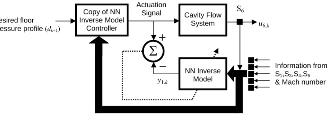
Due to its simplicity, our first trials for training a neurocontroller utilize the direct synthesis approach. We consider a NN structure y1,k+1 = NNC(dk+1, u6,k, u5,k, u3,k), provide some history of the sensory information and ask for

the control signal leading to the specified transition. Note that dk+1 refers to the signal we would like to observe at S6,

i.e. the desired floor pressure signal, the synthesis of which is to be explained (see section VI, Figure 15). In the training phase of the neurocontroller, we use dk+1=u6,k+1. We used a sampling rate of 50 kHz and LM algorithm for

parameter adjustment. The neurocontroller has 4 inputs, a single hidden layer with 7 neurons having hyperbolic tangent activation functions, and a single linear output neuron. We considered only the Mach 0.30 flow for the controller training, and we choose 49,000 successive measurements in total. The training took less than 5 minutes and gave the training performance illustrated in Fig. 10. The mean squared error decreases to a value of approximately 7⋅10-4 _{very quickly. Figure 11 depicts the corresponding time-domain results where we used a}

different set of 49,000 lines of test pairs to compare y1,k+1 and u1,k+1 and, based on the small value of the

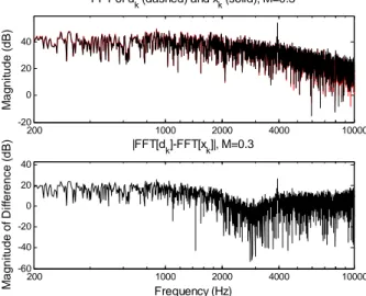
discrepancies between these quantities, we conclude that the neurocontroller performs satisfactorily and has a good representational capability. A better performance indicator is the similarity of Fast Fourier Transform (FFT) plot of the NN response (y1,k) and its desired value (u1,k), which has already been recorded during data collection.

Furthermore, the FFT of the difference between the involved signals is a good metric for assessing the performance. The results are shown in Fig. 12 and support the theoretical claims of this paper. The neural controller is trained for some ensemble of data and it is used to estimate some other ensemble that has been obtained from the same data-recording process.

These promising results for the NN based emulator and controller warranted a test to be done in real-time. We observe that our goals can be achieved with structurally very simple NNs. This is particularly important since the real-time implementation cost can be significantly reduced by off-line training of the NNs.

At this stage, it is useful to emphasize that a neurocontroller obtained as discussed above may not represent satisfactory closed loop performance but it is clearly a good initialization for on-line tuning schemes exploiting the indirect synthesis method illustrated in Fig. 9.

Finally, the identifiability and generalizability with a single NN is consistent with the physical evidence that the phenomenon taking place inside the test section has a coherent behavior at different Mach numbers (Samimy et al. 2004).

VI. Experimental Results

In this section, we summarize some preliminary results observed in the real-time experimental implementation of the NN emulator and of the directly-synthesized NN control schemes described above.

Figure 13 shows the Simulink block diagrams we used to implement the NN emulator (top) and the NN controller (bottom) in the dSPACE system used in our experiments. Figure 14 illustrates the ability of the NN emulator trained as explained in section IV in reconstructing the signal from pressure transducer S6 in the middle of

the cavity floor. Top Fig. 14 shows the simultaneously acquired transducer signal (thin line) and the NN emulator signal (thick line) for the unforced resonant Mach 0.30 flow. Middle and bottom Fig. 14 show similar signals for the Mach 0.3 flow respectively with OpFF sinusoidal forcing at 3920 Hz , 4 Vrms and with white noise forcing at 6 Vrms.

In all cases the signal reconstructed by the NN emulator matches very well the actual signal recorded by the pressure transducer S6. Both signals are very similar and almost perfectly match in amplitude and phase. Analogous results,

not shown here, were observed also using the NN emulator at other Mach numbers between 0.25 and 0.4 both without and with different types of forcing. This is a very promising result and indicates that a NN emulator with appropriate structure and training is capable to replicate the characteristics of a dynamic system like the one studied here.

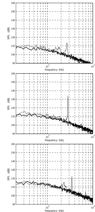
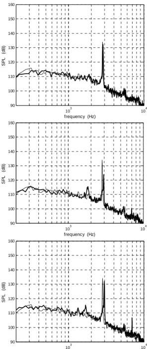
We also tested the real-time behavior of the directly-synthesized NN controller. As a preliminary step to this aim, we selected two suitable reference signals for the NN controller. The first is the zero signal, corresponding to absolute absence of pressure fluctuations, which we had already used as a reference in the PP control scheme (Debiasi et al. 2004b). The second is a white noise signal amplified by a gain varying linearly with Mach number and filtered by a 1st _{order low-pass filter with cutoff frequency of 1000 Hz. This signal accurately describes the}

background noise of the flow that would be measured in the facility in absence of the cavity-flow resonance phenomena as illustrated in Fig. 15 for the Mach 0.25, 0.30, and 0.35 cases.

Figure 16 illustrates the effect of the NN controller with the latter reference signal on the Mach 0.30 flow. In all figures, the thin line represents the baseline, unforced Mach 0.30 resonant flow, whereas the thick line is the same

flow with NN control at increasing actuation voltage levels. Top Fig. 16 is the effect of control with actuation voltage matching the control signal produced by the NN controller. The voltage of this signal, 0.2 Vrms, is very low

and as a result the effect of control is negligible and the resonant peak remains practically unchanged. Increasing the actuation signal to higher level, 1.6 Vrms, produces a 20 dB reduction of the resonant peak at the expense of the

excitation of a sideband peak at about 2950 Hz which is 9 dB lower than the original resonant tone, center Fig. 16. This decrease is also accompanied by the excitation of the second Rossiter mode of this flow as evidenced by the appearance of a small peak at about 1850 Hz. Similar results were observed by Samimy et al. (2004) when using linear controllers for this flow. Increasing the actuation voltage strengthens the sideband peak while shifting it to slightly higher frequencies. Bottom Fig. 16 shows this effect for actuation voltage 5.3 Vrms. Analogous results, not

shown here, were obtained using the zero signal as a reference signal for the NN controller.

A closer look at the results presented indicate that the neural controller, though it affects the flow, does not function as it is supposed to do. If the control gain is increased, as shown in center Fig. 16, the NN controllers have the potential for reducing the cavity flow resonance, but further work is necessary in order to improve its effectiveness. One reason for the obtained unsatisfactory result is the number of different cases used in the training. Few different rms excitation levels (in volts) and few different excitation frequencies have been utilized and it is seen that a minimum of the cost surface is reachable as shown by Fig. 10. Our research plan is to cover a richer set of training set to increase the representational content of the training data.

VII. Conclusions

This paper reports the use of NNs in flow identification and control applications. An experimental facility making it possible to conduct flow control research has been used and attempts have been made to address several questions that could be raised when tackling with NN use in dynamical systems. These questions and issues are summarized below.

• How many hidden layers are required?

• How many neurons should each hidden layer have? • Which activation function is needed?

• How many training samples are sufficient?

• Given the training data and network configuration, which learning algorithm best fulfills the needs?

• Regarding the application in hand, what delay depth for each sensor leads to minimal and useful neural model? • What is the applicable/affordable maximum delay depth?

• What is the lowest possible sampling frequency?

• Is the direct synthesis of a NN controller satisfactory in real time? Or do we need further improvement? • What is the relation between NN specific terms and the peak reduction performance in real time?

The focus of this research was not to address the first five, which are specific to the neurocomputing and for which the common answer is gaining insight by trial-and-error. Yet, a set of satisfactorily guiding answers to these questions are available in the presented discussion. Regarding the questions on sensor locations, relevant delay depths, and the sampling frequency, the results obtained in this work demonstrate that a delay depth of 3 is enough for devising an emulator, and finite number of sensors is sufficient to rebuild the response. Obviously, if the delay depth increases or if the number of sensors increases a better emulator might be obtained at the cost of increasing the computational complexity. Furthermore, a sampling frequency an order of magnitude larger than the phenomena is sufficient to obtain a convergent neurocontroller training as it captures the essential physical properties taking place inside the test section.

A neural emulator and a directly-synthesized neurocontroller were tested in real time in the experimental setup. The results indicate that the emulator can accurately reproduce a reference signal measured in the cavity floor at different Mach numbers and under different flow forcing conditions. Regarding the neurocontroller, the performance is not found to be satisfactory. Among many different controller structures and training MSE levels, the tested neural controllers have not caused a considerable peak reduction as the desired signal in Figure 15 prescribes. A reason for this may be the representational insufficiency of the signals used in the training phase to attain a desired floor pressure signal as in Figure 15. One should remember that the training phase is an open-loop and off-line mechanism that does not have the effects of closed-loop dynamics. Thus a training that takes place in closed loop might produce more meaningful data and a more effective neural controller. Although not tested in this study, the indirect synthesis mechanism illustrated in Figure 9 constitutes the future work of this research.

Acknowledgments

This work is supported in part by the AFRL/VA and AFOSR through the Collaborative Center of Control Science (Contract F33615-01-2-3154).

The authors would like to thank Drs. James Myatt, James DeBonis, and R. C. Camphouse, and Xin Yuan, James Malone and Jesse Little for fruitful discussions.

References

Cattafesta III, L. N., Garg, S., Choudhari, M., and Li, F., “Active Control of Flow-Induced Cavity Resonance”, AIAA Paper 97-1804, June 1997.

Debiasi, M. and Samimy, M., “Logic-Based Active Control of Subsonic Cavity Flow Resonance,” AIAA Journal, Vol. 42, No. 9, pp. 1901-1909, September 2004a.

Debiasi, M., Little, J., Malone, J., Samimy, M., Yan, P., and Özbay, H., “An Experimental Study of Subsonic Cavity Flow – Physical Understanding and Control,” AIAA Paper 2004-2123, June 2004b.

Efe, M. Ö., Debiasi, M., Özbay, H., and Samimy, M., “Modeling of Subsonic Cavity Flows by Neural Networks,” Int. Conf. on

Mechatronics (ICM’04), June 3-5, Istanbul, Turkey, pp.560-565, 2004.

Efe, M. Ö., “Identification and Control of Nonlinear Dynamical Systems Using Neural Networks,” M.Sc. Thesis, Bogazici University, 1996.

Faller, W. E., Schreck, S. J., and Luttges, M. W., “Real-Time Prediction and Control of Three Dimensional Unsteady Separated Flow Fields Using Neural Networks,” AIAA Paper 94-0532, January 1994.

Fan, X., Hofmann, L., and Herbert, T., “Active Flow Control with Neural Networks,” AIAA Paper 93-3273, July 1993.

Giralt, F., Arenas, A., Ferre-Gine, J., Rallo, R., and Kopp, G. A. , “The simulation and interpretation of free turbulence with a cognitive neural system,” Physics of Fluids, Vol. 12, No. 7, pp. 1826-1835, 2000.

Hagan, M. T. and Menhaj, M. B., “Training Feedforward Networks with the Marquardt Algorithm”, IEEE Transactions on

Neural Networks, Vol. 5, No. 6, pp. 989-993, November 1994.

Haykin, S., (1994). Neural Networks, Macmillan College Printing Co., New Jersey, 1994.

Jacobson, S. A. and Reynolds, W. C., “Active Control of Boundary Layer Wall Shear Stress Using Self-Learning Neural Networks,” AIAA Paper 93-3272, July 1993.

Jang, J.-S. R., Sun, C.-T., and Mizutani, E., Neuro-Fuzzy and Soft Computing, Prentice-Hall, New Jersey, 1997.

Kawthar-Ali, M. H. and Acharya, M., “Artificial Neural Networks for Suppression of the Dynamic Stall Vortex over Pitching Airfoils,” AIAA Paper 96-0540, January 1996.

Kim, J., “Control of Turbulent Boundary Layers,” Physics of Fluids, Vol. 15, No. 5, pp. 1093-1105, 2003.

Narendra K. S. and Parthasarathy, K. “Identification and Control of Dynamical Systems Using Neural Networks”, IEEE

Transactions on Neural Networks, Vol. 1, No. 1, pp. 4-27, 1990.

Lee, C., Kim, J., Babcock, D., and Goodman, R. “Application of Neural Networks to Turbulence Control for Drag Reduction,”

Physics of Fluids, Vol. 9, No. 6, pp. 1740-1747, 1997.

Rossiter, J. E., “Wind Tunnel Experiments on the Flow Over Rectangular Cavities at Subsonic and Transonic Speeds”, RAE Tech. Rep. 64037, 1964 and Aeronautical Research Council Reports and Memoranda No. 3438, October 1964.

Rumelhart, D. E., Hinton, G. E., and Williams, R. J., “Learning Internal Representations by Error Propagation”, in D. E. Rumelhart and J. L. McClelland, eds., Parallel Distributed Processing: Explorations in the Microstructure of Cognition, Vol. 1, pp. 318-362, MIT Press, Cambridge, M.A., 1986.

Samimy, M., Debiasi, M., Caraballo, E., Malone, J., Little, J., Özbay, H., Efe, M. Ö., Yan, P., Yuan, X., DeBonis, J., Myatt, J. H., and Camphouse, R. C., “Exploring Strategies for Closed-Loop Cavity Flow Control,” AIAA Paper 2004-0576, January 2004. Yan, P., Debiasi, M., Yuan, X., Caraballo, E., Efe, M. Ö., Özbay, H., Samimy, M., DeBonis, J., Camphouse, R. C., Myatt, J. H.,

Serrani, A., and Malone, J., “Controller Design for Active Closed-Loop Control of Cavity Flows”, AIAA Paper 2004-0573, January 2004.

Yuen, P. K. and Bau, H. H., “Controlling chaotic convection using neural nets – theory and experiments,” Neural Networks, Vol. 11, pp. 557, 1998.

Yuen, P. K. and Bau, H. H., “Optimal and adaptive control of chaotic convection – Theory and experiments,” Physics of Fluids, Vol. 11, No. 6, pp. 1435-1448, 1999.

KULITE TRANSDUCER

MAIN

FLOW W ACTUATOR OUTPUT _L

COMPRESSION DRIVER

2

3

4

5

6

2

4

5

6

3

Fig. 1: Scaled drawing of the experimental set up showing the incoming flow, the actuation location (at the receptivity location of the free shear layer formed over the cavity), and other geometrical details.

Fig. 2: Location of Kulite pressure transducers in the cavity flow. Location 1 (not shown in the figure) represents the excitation signal to the compression driver actuator.

Recorded information from S6 at time k+1 Auxiliary sensory readings at time kT, (k-1)T, ..., (k-m)T Excitation signal at time kT Neural Identifier

Σ

_

+

time k and the Mach number Estimated pressure reading at sensor 6 at time (k+1)T Output error Input Layer Hidden Layer Output ye La r

Fig. 3: The structure of the FNN with input-output definitions with T being the sampling period.

Fig. 4: Neural network based identification.

American Institute of Aeronautics and Astronautics 10 200 1000 2000 4000 10000 -20 0 20 40 M a gn it ude ( d B )

FFT of d_k(dashed) and x_k(solid), M=0.3

200 1000 2000 4000 10000 -60 -40 -20 0 20 40 Frequency (Hz) M a gni tu de of D if fe rence ( d B ) _|FFT[d k]-FFT[xk]|, M=0.3 1 2 3 4 5 6 7 8 -1 -0.5 0 0.5 1 F lo o r P re s s u re s d_kand x_k 1 2 3 4 5 6 7 8 -0.2 -0.1 0 0.1 0.2 Time (msec) Difference Between d_k and x_k

Fig. 7: Frequency domain results with Mach 0.30. Fig. 6: Time domain results with Mach 0.30.

Fig. 5: Time evolution of the mean square error over 147,420 patterns.

0 2 4 6 8 10 12 14 16 18 20 10-2 10-1 100 20 Epochs Performance is 0.00378559, Goal is 0.001

Observed Mean-squared Error Behavior over 147,420 patterns

American Institute of Aeronautics and Astronautics 11 Desired floor pressure profile Neural Emulator x(k+1)=f(…) Information from S1,S3,S4,S5

Σ

+

-

_

+

Σ

Fig. 10: The evolution of the mean squared error calculated over the entire set of data points. The solution implied by the data is obtained approximately after 25 epoches.

0 5 10 15 20 25 10-3 10-2 10-1 100 101 25 Epochs Performance is 0.000696438, Goal is 0.0001

Fig. 9: Indirect synthesis of a neural network controller. Fig. 8: Direct synthesis of a neural network controller.

Information from S1,S3,S4,S5

& Mach number

+

Σ

_

American Institute of Aeronautics and Astronautics 12 200 1000 2000 4000 10000 10 20 30 40 50 60 70 M a gn it ude ( d B )

FFT of Desired (dashed red) and Predicted (solid black) Signals

200 1000 2000 4000 10000 -100 -50 0 Frequency (Hz) M a gni tu de of D if fe rence ( d B ) _|FFT[u 1,k]-FFT[y1,k]|

Fig. 12: Top figure illustrates the FFT of the response of the NN controller together with the desired values read from the experimental data. The bottom figure depicts the FFT of the magnitude of the error between the desired value and the reconstructed value of the signal at sensor S1. The visualized data contain the

measurements for Mach 0.30 case.

Fig. 13: Simulink block diagrams of the NN emulator (top) and of the corresponding NN controller (bottom) for implementation in the dSPACE control system.

1 2 3 4 5 6 7 8 -5 0 5 C o nt ro l S ign al s

y_1,k+1(Black) and u_1,k+1(Red)

1 2 3 4 5 6 7 8 -0.1 -0.05 0 0.05 0.1 Time (msec) The Difference u_1,k+1-y_1,k+1

American Institute of Aeronautics and Astronautics 13 0 1 2 3 4 5 x 10-3 -0.8 -0.6 -0.4 -0.2 0 0.2 0.4 0.6 0.8 time (seconds) vo ltag e 0 1 2 3 4 5 x 10-3 -0.8 -0.6 -0.4 -0.2 0 0.2 0.4 0.6 0.8 time (seconds) vo ltag e 0 1 2 3 4 5 x 10-3 -0.8 -0.6 -0.4 -0.2 0 0.2 0.4 0.6 0.8 time (seconds) vo ltag e

Fig. 14: Timetraces of signal from cavity floor transducer (thin line) and of NN emulator response (thick line) of Mach 0.30 flow: without forcing (top); with OpFF sinusoidal forcing at 3920 Hz, 4Vrms (middle); white noise

forcing at 6 Vrms (bottom).

Fig. 15: Spectra of pressure transducer signal in the cavity floor (thin line) and of synthesized reference background noise (thick line) for resonant flow at: Mach 0.25 (top); Mach 0.30 (center); Mach 0.35 (bottom).

103 104 90 100 110 120 130 140 150 160 frequency (Hz) SP L ( d B ) 103 104 90 100 110 120 130 140 150 160 frequency (Hz) SP L ( d B ) 103 104 90 100 110 120 130 140 150 160 frequency (Hz) SP L ( d B )

103 104 90 100 110 120 130 140 150 160 frequency (Hz) SP L (dB ) 103 104 90 100 110 120 130 140 150 160 frequency (Hz) SP L (dB ) 103 104 90 100 110 120 130 140 150 160 frequency (Hz) SP L (dB )

Fig. 16: Effect of amplification of NN control signal. Thin line is spectrum of cavity floor signal of the baseline Mach 0.30 resonant flow; thick line is analogous spectrum with NN control at: voltage matching 0.2 Vrms (top); 1.6 Vrms (middle);

5.3 Vrms (bottom).