H (formula) based filtering for systems with time delays and application to vehicle tracking

H

BASED FILTERING FOR SYSTEMS WITH TIME

DELAYS AND APPLICATION TO VEHICLE

TRACKING

a thesis

submitted to the department of electrical and

electronics engineering

and the institute of engineering and sciences

of bilkent university

in partial fulfillment of the requirements

for the degree of

master of science

By

Mehmet Sami EZERCAN

August 2007

I certify that I have read this thesis and that in my opinion it is fully adequate, in scope and in quality, as a thesis for the degree of Master of Science.

Prof. Dr. Hitay ¨Ozbay(Supervisor)

I certify that I have read this thesis and that in my opinion it is fully adequate, in scope and in quality, as a thesis for the degree of Master of Science.

Assist. Prof. Dr. Defne Akta¸s

I certify that I have read this thesis and that in my opinion it is fully adequate, in scope and in quality, as a thesis for the degree of Master of Science.

Prof. Dr. M¨ubeccel Demirekler

Approved for the Institute of Engineering and Sciences:

Prof. Dr. Mehmet Baray

ABSTRACT

H

BASED FILTERING FOR SYSTEMS WITH TIME

DELAYS AND APPLICATION TO VEHICLE

TRACKING

Mehmet Sami EZERCAN

M.S. in Electrical and Electronics Engineering

Supervisor: Prof. Dr. Hitay ¨

Ozbay

August 2007

In this thesis, the filtering problem for linear systems with time delay is studied. The standard mixed sensitivity problem is investigated and the duality between

H∞ control problem and H∞ filtering problem is established. By using this

duality an alternative H∞ filtering method is proposed.

An optimum H∞ filter is designed for single output system. However the

pro-posed technique does not only work for single delay in the measurement but also works for multiple delays in both state and measurement if the linear system has more than one outputs with delay. For this case, different suboptimal filters are designed.

This work also deals with an important aspect of tracking problems appearing in many different applications, namely state estimation under delayed and noisy measurements. A typical vehicle model is chosen to estimate the delayed state and the performances of the designed filters are examined under several scenarios based on different parameters such as amount of delays and disturbances.

Keywords: Time Delay Systems, State Estimation, H∞ Filtering, Vehicle

¨

OZET

ZAMAN GEC˙IKMEL˙I S˙ISTEMLER ˙IC

¸ ˙IN H

TABANLI

KEST˙IR˙IM VE ARAC

¸ TAK˙IP PROBLEM˙INE UYGULANMASI

Mehmet Sami EZERCAN

Elektrik ve Elektronik M¨uhendisli¯gi B¨ol¨um¨u Y¨uksek Lisans

Tez Y¨oneticisi: Prof. Dr. Hitay ¨

Ozbay

A˜gustos 2007

Bu tez kapsamında zaman gecikmeli do˜grusal sistemler i¸cin kestirim problemi ¨uzerinde ¸calı¸sılmı¸stır. Standart karı¸sık hassasiyet problemi incelenmi¸s, burada anlatılan H∞ kontrol problemi ile ¨uzerinde ¸calı¸sılan kestirim problemi arasında

benzerlik kurulmu¸stur. Bu benzerlik kullanılarak alternatif bir kestirim metodu ¨onerilmektedir.

Tek bir zaman gecikmesine sahip bir sistem i¸cin optimum s¨uzge¸c tasarlanmı¸stır. Bununla beraber ¨onerilen y¨ontem birden ¸cok gecikmeli ¸cıktısı olan sistemlerde sadece ¨ol¸c¨umde yer alan tek bir gecikme i¸cin de˜gil, hem konumda hem de ¨ol¸c¨umde yer alan birden fazla gecikme i¸cin ¸calı¸sabilmektedir. B¨oyle bir durumda farklı alt optimum s¨uzge¸cler tasarlanmı¸stır.

Bu ¸calı¸smada ayrıca bir¸cok uygulamada da g¨or¨ulebilecek olan izleme problemi yani gecikmeli ve g¨ur¨ult¨ul¨u ¨ol¸c¨umlerle konum kestirimi ¨uzerine ¸calı¸sılmıstır.

¨

Ornek bir ara¸c modeli se¸cilmi¸s ve gecikmedeki farklılık ve benzeri de˜gi¸sik senary-olarda, tasarlanan s¨uzgecin performansı test edilmi¸stir.

Anahtar Kelimeler: Zaman gecikmeli sistemler, Konum kestirimi, H∞ s¨uzge¸c,

ACKNOWLEDGMENTS

I would like to express my gratitude to Prof. Dr. Hitay ¨Ozbay for his supervision, support and guidance throughout my graduate studies.

I would like to thank committee members Assist. Prof. Dr. Defne Akta¸s and Prof. Dr. M¨ubeccel Demirekler for reading and commenting on this thesis. I would like to thank my family for their endless support, encouragement and trust throughout my life.

I would like to express my special thanks to Canan Karamano˘glu for her great support, encouragement and understanding while writing this thesis.

I would also like to thank Mehmet K¨oseo˘glu and Hande Do˘gan for their under-standing and support whenever I needed.

At last, I would like to thank my colleagues at Aselsan Inc. for their moral support.

Contents

1 INTRODUCTION 1

1.1 Estimation & Filtering . . . 1

1.2 Optimal Filtering . . . 3

1.3 H∞ Optimal Filtering . . . 4

1.4 Time Delay Systems . . . 5

1.5 State Estimation for Time Delay Systems . . . 6

1.5.1 H∞Techniques for State Estimation for Time Delay Systems 6 1.5.2 Other Techniques for State Estimation for Time Delay Sys-tems . . . 8

1.6 Thesis Contribution and Organization . . . 10

2 FILTERING VIA DUALITY BETWEEN CONTROL AND ES-TIMATION PROBLEMS 11 2.1 System Architecture . . . 11

2.3 Mixed Sensitivity Control Problem . . . 15

2.4 Solution . . . 17

2.4.1 Suboptimal Approach-I . . . 18

2.4.2 Suboptimal Approach-II . . . 19

3 APPLICATION TO VEHICLE TRACKING PROBLEM 21 3.1 Tracking Problem . . . 21

3.1.1 Moving Vehicle Model . . . 22

3.2 Illustrative Examples and Simulation Results . . . 25

3.2.1 Single Delay in Output . . . 26

3.2.2 Multiple Delay in Output . . . 39

3.2.3 Delay in both State and Output . . . 40

3.3 Comparative Results . . . 42

3.3.1 Kalman Filter Approach . . . 42

3.3.2 Mirkin’s H∞ Suboptimal Filter Approach . . . 46

List of Figures

1.1 Estimation Problem in General . . . 3

2.1 Dynamic System Model for Estimation . . . 12

2.2 Feedback Control System . . . 16

3.1 Process Noise w(t) . . . 23

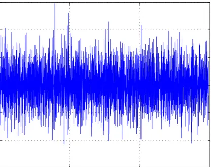
3.2 Measurement Noise v(t) . . . 24

3.3 Original Trajectory to be Estimated . . . 24

3.4 z(t) − y(t) for Case 1 . . . 29

3.5 Estimation Error (z(t) − ˆz(t)) for Case 1 . . . 29

3.6 z(t) − y(t) for Case 2 . . . 30

3.7 Estimation Error (z(t) − ˆz(t)) for Case 2 . . . 31

3.8 z(t) − y(t) for Case 3 . . . 32

3.9 Estimation Error (z(t) − ˆz(t)) for Case 3 . . . 32

3.10 Measurement Noise associated with a High Pass Filter . . . 33

3.12 Estimation Error (z(t) − ˆz(t)) for Case 4 . . . 34

3.13 Estimation Error (z(t) − ˆz(t)) for the System with Actual Delay is 1 35

3.14 Estimation Error (z(t) − ˆz(t)) for the System with Actual Delay is 3 36

3.15 z(t) − y(t) for the system with ε = 0.2 . . . 37 3.16 Estimation Error (z(t) − ˆz(t)) for the system with ε = 0.2 . . . . 37

3.17 z(t) − y(t) for the system with ε = 10 . . . 38 3.18 Estimation Error (z(t) − ˆz(t)) for the system with ε = 0.2 . . . . 38

3.19 γ1+ γ2 for Suboptimal Filter Approach . . . 39

3.20 z(t) − y(t) if the State has Time Delay in addition to that in Measurement . . . 41 3.21 Estimation Error (z(t) − ˆz(t)) if the State has Time Delay in

ad-dition to that in Measurement . . . 41 3.22 Estimation Error (z(t) − ˆz(t)) for the Kalman Filter with initial

state with process noise information . . . 46 3.23 Estimation error (z(t) − ˆz(t)) for t ∈ [0, 25] of Case 1 in Section

3.2.1 . . . 47 3.24 Estimation Error (z(t) − ˆz(t)) for the Kalman Filter without

pro-cess noise information . . . 48 3.25 Estimation Error (z(t) − ˆz(t)) for the Kalman Filter without

pro-cess noise information . . . 49 3.26 Dynamic System for the Mirkin’s Approach . . . 50 3.27 Estimator to be Designed by Mirkin’s Approach . . . 50

3.28 Estimation Error (z(t) − ˆz(t)) for Case 1 with Mirkin’s Approach 51

Chapter 1

INTRODUCTION

In this thesis we consider H∞filtering for systems with time delay. We use duality

between control and estimation problems to propose a new structure for H∞

based filters and apply to vehicle tracking under delayed and noisy measurements. In this chapter we give an overview of existing literature on estimation and filtering as well as on systems with delay and H∞ techniques.

1.1

Estimation & Filtering

Estimation is the calculated approximation of a result which is usable even if input data may be incomplete, uncertain, or noisy. Estimation is defined as the process of inferring the value of a quantity of interest from indirect, inaccurate and uncertain observations, [21].

Some examples of estimation are:

• Statistical inference [40]

• Application of control to a plant in the presence of uncertainty (parameter

identification, state estimation and stochastic control) [41]

• Determination of model parameters for predicting the state of a physical

system (system identification) [39]

• Determination of characteristics of a transmitted message from

noise-corrupted observation of the received signal (communication theory) [38]

• Determination of some parameters or characteristics of a signal or image

(signal processing) [37]

In general, estimation can be classified into two categories related to the variable to be estimated.

• Parameter estimation for linear time invariant (LTI) systems

• State Estimation (Parameter estimation for time varying systems can be

cast into this framework)

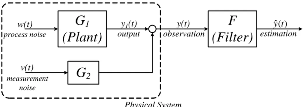
While parameter estimators for LTI systems deal with a time invariant quan-tity, state estimators are used in dynamic systems evolving in time and are more general than parameter estimators. In this thesis we will deal with state es-timaton which is illustrated by Figure 1.1. The only part of the system that the estimator can access is the measurement which is affected by the measure-ment noise where the other parts are fixed transfer matrices. Estimation can be classified into three groups according to its nature and purpose [21]:

Filtering is the estimation of the current state of a dynamic system and provides an estimate of the output based on all data up to the current time.

Prediction is the estimation of the state ahead of the observed data. Pre-diction provides an estimate of the output at time k based on the data up to an earlier time j < k.

G

(Plant)

F

(Filter)

G

Figure 1.1: Estimation Problem in General

Smoothing is the estimation of the state behind of the observed data that are ahead in time of the estimate. Smoothing provides an estimate of the output at time k based on the data up to j > k.

Since we deal with real time estimation in this work we will use the term filtering. Actually the filter is a procedure of looking at a collection of data taken from a system or process. The term filtering mainly means that the process of removing undesired signals from the system, namely filtering the noise out.

The main concerns for someone, who does estimation, are the following [21]:

• A basic model of the system has to be available with unknown states to be

estimated.

• Physical data are required to reduce the effect of measurement errors. • In order to make the most accurate estimation, the residuals (difference

between observation and estimation) should be as small as possible but one does not have control over this physical constraint.

1.2

Optimal Filtering

Optimal filtering is an innovative technique for detecting a signal against a back-ground of noise or natural variability. While using optimal estimation techniques

someone has a model for some form of data that he or she observes or measures and also has an error criterion to minimize. Optimal estimation makes the best utilization of the data and the knowledge of the system and the disturbances under the optimization of some criterion. On the other hand, optimal estimation techniques can be sensitive to modeling errors and also computationally expen-sive. So it is very important to have a clear understanding of the assumptions under which an algorithm is optimal and also it is very important how these assumptions relate to real world.

1.3

H

Optimal Filtering

In H∞ filtering, H∞ norm of the system which reflects the worst case gain of

system is minimized. One does not need the exact knowledge of the statistics of the exogenous signals while designing an H∞ optimal estimator. This

estima-tion procedure ensures that the L2 induced gain from the noise signals to the

estimation error will be less than a prescribed γ level, where the noise signals are arbitrary energy-bounded signals. In the H∞ setting, the exogenous input

signal is assumed to be energy bounded rather than Gaussian white noise. Figure 1.1 is the general scheme of estimation. H∞ filtering for such a system is made

performing the following expressions:

y1 = G1w y = y1 + G2v

Exogenous signals w and v prevent handling the measurement correctly. So we need to filter the measurement, y, with a filter denoted as F .

ˆ

y = F y

Then the error between the output and estimated measurement is called esti-mation error of which L2 norm over L2 norm of noise signals will be less than

prescribed γ. e = F y − y1 = (F − I)G1w + F G2v γ = sup kek2 k   w v   k2 such that   w v   6= 0.

1.4

Time Delay Systems

Time-delay systems appear naturally in many engineering applications and, in fact, in any situation in which transmission delays cannot be ignored. Therefore, their presence must be taken into account in a realistic filter design. Moreover, stability and noise attenuation level guaranteed by filter design without consider-ing time delays may collapse in the presence of non-negligible time delays. Time delays arise in several signal processing related problems, such as, echo cancella-tion, local loop equalizacancella-tion, multipath propagation in mobile communications, and array signal processing.

Time delays often also appears in many control systems (such as aircraft, chemical or process control systems) either in the state, the control input, or the measurements. Unlike ordinary differential equations, delay systems are infinite dimensional in nature and time-delay is, in many cases, a source of instabil-ity. The stability issue and the performance of control systems with delay are, therefore, both of theoretical and practical importance [36].

For a brief history of time delay systems, see [36] where it is mentioned that the delay equations were first considered in the literature in the XVIII century. Also it is mentioned in the same paper that systematic method study has began and Lyapunov’s method was developed for stability of delay systems until 50’s in XX century. Since 1950s, the subject of delay systems or functional differential

equations has received a great deal of attention in Mathematics, Biology and Control Engineering.

Over the past decade, much effort has been invested in the analysis and synthesis of uncertain systems with time-delay. Based on the Lyapunov the-ory of stability, various results have been obtained that provide, for example, finite-dimensional sufficient conditions for stability and stabilization. Departing from the classical linear finite-dimensional techniques which apply Smith predic-tor type designs, the new methods simultaneously allow for delays in the state equations and for uncertainties in both the system parameters and the time de-lays. During the early stages, delay-independent results were obtained which guarantee stability and prescribed performance levels of the resulting solutions. Recently, delay-dependent results have been derived that considerably reduce the overdesign entailed in the delay-independent solutions. In the present issue, new results are obtained for various control and identification problems for delay systems. These results are based either on Lyapunov methods or on frequency domain considerations.

In the next section we will focus on H∞ filtering for time delay systems.

1.5

State Estimation for Time Delay Systems

1.5.1

H

Techniques for State Estimation for Time Delay

Systems

Many different H∞ filtering techniques have appeared in the literature. All of

them try to develop methodologies which ensure a prescribed bound on L2

in-duced gain from noise signals to filtering error [4]-[15]. In this scope following Luenberger observer type filter is developed depending on a derived version of

bounded real lemma [5] and depending on a descriptor model transformation, Park’s inequality, for the bounding of cross terms [6]. Some of them includes polytopic uncertainties in all matrices [6], [10], [11]. Consider a dynamic system as below: ˙x(t) = Ax(t) + m X i Aix(t − hi) + Bw(t) y(t) = Cx(t) + m X i Cix(t − hi) + Dw(t)

where x(t) is the state vector, y(t) is the measurement output vector, h is the fixed, known delay and w(t) is the L2 disturbance vector (w ∈ L2[0, ∞]).

Luen-berger type observer for the above system is given by the following dynamical system: ˙ˆx(t) = Aˆx(t) +Xm i Aix(t − hˆ i) − L(ˆy(t) − y(t)) ˆ y(t) = C ˆx(t) + m X i Cix(t − hˆ i)

where ˆx(t) is the estimated state of x(t), ˆy(t) is the estimated output of y(t) and L is the observer gain matrix. The estimated error, defined as e(t) = x(t) − ˆx(t),

obeys the following dynamical system: ˙e(t) = (A − LC)e(t) +

m

X

i

(Ai− LCi)(t − hi) + (B − LD)w(t)

Then the γ observer for this system is designed under the conditions:

1. limt→∞e(t) → 0 for w(t) ≡ 0

2. kTewk∞≤ γ

where Tew is the transfer function from disturbance w to the estimation error e

and γ > 0. Now the problem is to reach L which is found by solving some set of linear matrix inequalities (LMI) and algebraic riccati equations in [5]-[9] as below:

L = 1 εP

where P is the solution of linear matrix inequalities or algebraic riccati equations. Both instantaneous and multiple-time delayed measurements using the tech-nique that re-organizes innovation analysis approach in Krein space is studied in [12]. It also gives the results in terms of the solutions of Algebraic Riccati and Matrix Differential Equations.

Full order and reduced order filters are designed for discrete time linear sys-tems with delay [13], [14]. In order to design these type of filters LMI’s are used similar to the ones in continuous time systems.

We should indicate that most of the above mentioned techniques involving LMIs are suboptimal in the sense that the filter can be obtained under the condition that the LMIs are solvable. In most situations the optimal performance level cannot be achieved. Besides the frequency domain method proposed in this paper, there are some time domain state-space based techniques leading to optimal H∞ filters, see e.g. [17], [16]. In [16] a lifting technique is used to solve

the associated Nehari problem (see Chapter 2 below). In [17], Mirkin solves the problem by parameterizing all solutions of the non-delayed problem and finding the ones which solve the delayed problem. This approach involves solving Riccati equations and checking a spectral radius condition. Among all available methods for the solution of the H∞ suboptimal filtering problem under delayed and noisy

measurements, Mirkin’s approach [17] is the simplest. Moreover, his ”central” filter’s performance can get arbitrarily close to the optimum.

1.5.2

Other Techniques for State Estimation for Time

De-lay Systems

Although H∞ filtering technique is widely used method for time delay systems,

observers for systems with time delays in state variables both in continuous time [22] and in discrete time [23]. Also similar approach is developed in [24] not for single delay as in [22] and [23] but multiple delays in state variables. Motivated by the previous works, similar but extended types of observers are developed [32]. Functional, reduced order and full order observers with and without internal delays are considered. However only the delay in the state equation is considered while designing observers. The observer converges, with any prescribed stability margin, to any number of linear functionals when some conditions are met in [33].

A robust observer is designed in [25] using LMI’s. In order to provide the stability of observer it can be designed in two steps of which first step is to design a linear feedback control [29]. Then two Luenberger type observers are designed in the second step. Sufficient conditions are given in the form of Linear Matrix Inequalities.

State observers for systems with nonlinear disturbances where the non-linearities satisfy the Lipschitz conditions is considered in [34]. It is shown that the observation error is globally exponentially stable.

H2 filtering for linear systems with time delays is issued in [26]-[28]. Since the

filtering problem for time delay systems problem is infinite dimensional in nature, an attempt is made to develop finite dimensional methods that will guarantee a preassigned estimation accuracy. They give the sufficient conditions in the form of Linear Matrix Inequalities.

Kalman filter approach is extended to the case in which the linear system is subject to norm-bounded uncertainties and constant state delay then a robust estimator is designed for a class of linear uncertain discrete-time systems [30]. Estimation error covariance is guaranteed to lie within a certain bound for all admissible uncertainties solving two Riccati Equations. In this framework [20]

discusses trade off between optimality and computational burden of the filter and develops a method based on ”extrapolating” the measurement to present time using past and present estimates of the Kalman filter and calculating an optimal gain for this extrapolated measurement.

1.6

Thesis Contribution and Organization

In the remaining parts of the thesis, using the frequency domain representations, we provide an alternative method to compute the H∞ optimum filter directly.

First, by using the duality between filtering and control, the problem at hand is transformed to a robust controller design for systems with time delays. The skew Toeplitz method developed earlier for the robust control of infinite dimensional systems, [1], [2], [3], is used to solve the H∞ optimal filtering problem.

In Chapter 2, H∞ estimation problem is described in detail and duality

be-tween estimation problem and standard mixed sensitivity H∞ control problem

is given. The solution process that is used in this work is mentioned and some number of approaches are developed for the solution. Chapter 3 includes vehicle tracking problem definition with the reason why we have chosen this problem as well as the illustrative examples and comparative results with the previous methods. Chapter 4 concludes the work and proposes some future work.

Chapter 2

FILTERING VIA DUALITY

BETWEEN CONTROL AND

ESTIMATION PROBLEMS

In this chapter a solution for H∞ filtering problem is proposed establishing the

duality between control and estimation problems. First the system for which the estimator will be designed is clarified and then the control problem is shortly mentioned and the solution is given at last.

2.1

System Architecture

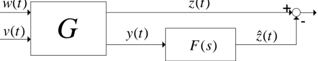
Consider the linear system in Figure 2.1 with multiple time delays in state and output variables as described in (2.1), (2.2) and (2.3).

˙x(t) = A0x(t) + k X i=1 Aix(t − hi) + Bw(t) (2.1) yj(t) = Cjx(t − hj) + Djvj(t) j = 1, . . . , l (2.2)

+

-)

(t

z

e

)

(t

w

)

(t

v

_y

_(t

₎

_z

_{ˆ t}

₍

₎

)

(s

F

G

Figure 2.1: Dynamic System Model for Estimation

z(t) = Lx(t) (2.3)

where x(t) ∈ Rn _{is the state vector, y}

j(t) ∈ Rp is jth output vector, z(t) is the

state variable to be estimated, w(t) and v(t) are process noise and measurement noise respectively. Time delays hiand hj are assumed to be known. The matrices

A0, Ai, B, Cj, Dj and L are also known. Each sensor output available for filtering

is described in (2.2).

Assumption: All the sensors that give information about the state are iden-tical. They have all same characteristics other than the delays that differ due to the other factors such as distance and communication link properties. Therefore we assume that hj > 0 for all j and Cj’s are same with each other and also with

L, namely:

C1 = C2 = C3 = ... = Cl= L = C (2.4)

Then (2.2) turns into;

yj(t) = Cx(t − hj) + Djvj(t) j = 1, . . . , l (2.5)

2.2

H

Filtering Problem

The term estimator is used for the function which gives the estimated value that we look for. For the system above, we will design an estimator in order to estimate z(t) and this estimator must minimize the estimaton error which is the difference between estimate and the objective function, z(t). Transfer functions

in (2.1) and (2.2) are found as following: Taking the Laplace Transform of both sides of (2.1) gives sX(s) = A0X(s) + k X i=1 e−his_A iX(s) + BW (s) (2.6)

where the Laplace Transform of x(t) is X(s) and of x(t − h) is e−hs_{X(s). Then}

the transfer funcion from w to state x is

X(s) = R(s)BW (s) (2.7) where R(s) = (sI − A0− k X i=1 Aie−his)−1 (2.8)

The transfer function to the output is found as below:

Yj(s) = Ce−hjsX(s) + DjVj(s) (2.9)

Using X(s) obtained from (2.7) turns (2.9) into

Yj(s) = Ce−hjsR(s)BW (s) + DjVj(s) (2.10)

In these type of systems, time delays in state and output prevent handling the output directly. Due to the this fact we have to minimize the estimation error corresponding to the estimate ˆz(t), which is mainly composed of a filter

affecting on the output y(t) and expressed in frequency domain as ˆ Z(s) = l X j=1 Fj(s)Yj(s) (2.11)

Thus the estimation error is written and found by the following equations:

E(s) = Z(s) − ˆZ(s) = LX(s) − l X j=1 Fj(s)Yj(s) (2.13) = LR(s)BW (s) − l X j=1 Fj(s)(Ce−hjsR(s)BW (s) + DjVj(s))

Let us now assume that the measurement noise v is generated by a known coloring filter Wv, i.e. V (s) = Wv(s) ˆV (s), where ˆv(t) is an unknown finite energy signal.

Similarly, let w be an unknown finite energy signal. Then the estimation error is

E(s) = (I − l X j=1 Fj(s)e−hjs)P0(s)W (s) − l X j=1 Fj(s)DjWvVˆj(s) = h (I −Pl_j=1Fj(s)e−hjs)P0(s) −F1(s)D1(s)Wv . . . Fl(s)Dl(s)Wv i          W (s) ˆ V1(s) ... ˆ Vl(s)          = h (I − F(s)H(s))P0(s) −F(s)D(s) i  W (s) ˆ V(s)   _(2.14) where P0 = CR(s)B, L = C and F(s) = h F1(s) F2(s) ... Fl(s) i D(s) =          D1(s)Wv 0 0 0 0 D2(s)Wv 0 0 0 0 . .. 0 0 0 0 Dl(s)Wv          H(s) =          e−h1s e−h2s ... e−hls          (2.15) ˆ V(s) = h ˆ V1(s) ˆV2(s) ... ˆVl(s) iT D(s), D−1_{(s) are stable.}

Fj(s)’s are the filters that will be designed to eliminate the effect of hj’s for each

Then the L2 induced norm from external signals w and ˆv to the error e is γ = inf F ∈H∞k h (I − F(s)H(s))P0(s) −F(s)D(s) i k∞ (2.16)

Multi-input multi-output (MIMO) solution of filtering problem will be reached via (2.16). However let us reduce it to a simpler solution which is Single-input single-output (SISO) case

γj = inf F ∈H∞k ( 1 l − Fj(s)e−hjs)P0(s) −Fj(s)DjWv k∞ = sup ˆ v;w 6= 0 kejk2 k   w ˆ vj   k2 (2.17)

However multi output case brings a suboptimal solution in other words sum of the optimal solutions for each output do not go to an optimal filter in general solution because; γopt ≤ l X j=1 γj.

Clearly the following two conditions must be satisfied in order to have a finite

γj:

Fj(s) is stable, and

(1

l − Fj(s)e−hjs)P0(s) is stable (2.18)

2.3

Mixed Sensitivity Control Problem

The standard mixed sensitivity H∞ control problem associated with a stable

plant eP shown in Figure 2.2 can be defined as follows.

Transfer functions from the disturbance ew to ey and eu are:

C

~

P

~

w

w

y

~

u~

w

~

−

+ +

Figure 2.2: Feedback Control System

Tw→ee u = −W2C(1 + ee P eC)−1 (2.20)

The optimal H∞ controller design problem is:

minimize γ

subject to ( eP , eC) is stable, and

(2.21) γ = ||T e w→ 2 6 6 6 4 e y e u 3 7 7 7 5 ||∞ (2.22)

In order to find the smallest γ following is solved as below in case all the variables are constant (if not, transpose of that has to be solved):

inf e Q∈H∞ khW1(1 − eP eQ) − W2Qe i k∞ (2.23)

The free parameter eQ is obtained from the controller

e C = Qe 1 − eP eQ e Q = Ce 1 + eP eC.

The important point throughout this work is that the SISO result of the estima-tion problem (2.17) is the same problem with (2.23) provided that the following dualities are established:

W1(s) = P0(s) W2(s) = −I e P (s) = e−hjs_D−1 j Wv−1(s) e Q(s) = Fj(s)DjWv(s) (2.24)

2.4

Solution

The problem of Section 2.3 can be solved using the technique in [1] where an optimal controller is designed for the system in Figure 2.2 in the form of:

e

Copt(s) = Eγ0(s)md(s)

N0(s)−1Fγ0(s)L(s)

1 + mn(s)Fγ0(s)L(s)

(2.25) The plant P (s) admits a coprime inner/outer factorization of the form P (s) =

mn(s)No(s)/md(s) where md and mn are inner and No is outer. Set Eγo as

Eγo := µ W1(−s)W1(s) γ2 − 1 ¶ Then define Fγo = Gγo(s) nl Y k=1 s − ηk s + ηk

where η1, . . . , ηk are the poles of fW1(−s) and Gγo is minimum phase and

deter-mined from the spectral factorization

Gγo(s)Gγo(−s) :=

µ

1 − (W2(s)W2(−s)

γ2 − 1)Eγo(s)

¶₋₁

L(s) is composed of the form L(s) = L2(s)/L1(s) where L2(s) and L1(s) are the

polynomials which satisfy the interpolation conditions given in [1].

After deriving the controller expression it is easy to find dual filter equation that we desire:

e

2.4.1

Suboptimal Approach-I

Reconsider the estimation error under the special case restriction that is, ˆ vj = ˆvi = v E(s) = h (I −Pl_j=1Fj(s)e−hjs)P0(s) −F(s)D(s) i  W (s) ˆ V(s)  

where F(s), D(s) and ˆV(s) are defined by (2.15). Let ˆFj(s) = Fj(s)Dj(s)Wv

and eF (s) =Pl_j=1Fˆj(s) Then first part of the above expression becomes

h (I −Pl_j=1Fˆj(s)Dj−1(s)Wv−1e−hjs)P0(s) − eF (s) i = h (I − D−1 1 (s)Wv−1e−h1sF(s))P0(s) − eF (s) i where F(s) = ˆF1(s) + eF (s) − eF (s) + l X j=2 Fj(s)D1(s)D−1j (s)e−(hj−h1)s

Assume that h1 ≤ h2 ≤ . . . ≤ hl (If not, following operations can be modified

easily) E(s) = h (I − D₁−1(s)W−1 v e−h1sF (s))Pe 0(s) − eF (s) i  w v   + h D−1 1 (s)Wv−1e−h1s(I − D1(s)D2−1(s)e−(h2−h1)s) ˆF2(s)P0(s) 0 i  w v   ... + h D−1 1 (s)Wv−1e−h1s(I − D1(s)D−1l (s)e−(hl−h1)s) ˆFl(s)P0(s) 0 i  w v  

Now the problem will be solved in steps:

1. minimize k (I − D−1

1 (s)Wv−1e−h1sF (s))Pe 0(s) − eF (s) k∞ and find optimal

e

2. minimize kW0+ D−11 (s)Wv−1e−h1s(I − D1(s)D−12 (s)e−(h2−h1)s) ˆF2(s)P0(s)k∞

where W0 = (I − D1−1(s)Wv−1e−h1sF (s))Pe 0(s) and find optimal ˆF2(s).

3. minimize kW1+ D−11 (s)Wv−1e−h1s(I − D1(s)D−13 (s)e−(h3−h1)s) ˆF3(s)P0(s)k∞

where W1 = W0+ D−11 (s)Wv−1e−h1s(I − D1(s)D2−1(s)e−(h2−h1)s) ˆF2(s)P0(s)

and find optimal ˆF3(s).

4. . . .

Step 1 is the dual problem of the work solved before so eF (s) is found easily.

Step 2 and subsequent ones are more complicated than first step. They will also be solved by same technique, however some sort of extra works have to be done in order to obtain a solvable minimization problem.

2.4.2

Suboptimal Approach-II

Reconsider the estimation error equation (2.14):

E(s) = h (I − F(s)H(s))P0(s) −F(s)D(s) i  W (s) ˆ V(s)   .

Above expression can be written as sum of l expressions:

E(s) = l X j=1 h (αj − Fj(s)e−hjs)P0(s) −Fj(s)DjWv i  W (s) ˆ Vj(s)   _(2.26) where Pl_j=1αj = 1

Each error expression namely the estimation error of jth _{output is solved in}

order to find Fj(s) writing the L2induced norm from exogeneous signals to error: γj = inf F ∈H∞k (1 − α −1 j Fj(s)e−hjs)αjP0(s) −Fj(s)DjWv k∞ = sup ˆ v,w 6= 0 kejk2 k   w ˆ vj   k2 (2.27)

Optimal γj can be found easily using the method developed by dual control

problem. However solving l-decoupled SISO H∞ optimization problem gives a

suboptimal solution since sup ˆ v,w 6= 0 kejk2 k   w ˆ vj   k2 ≤ l X j=1 k (αj − Fj(s)e−hjs)P0(s) −Fj(s)DjWv k∞

which means the sum of optimal γj’s for each output is larger than the optimal

γ of the complete problem.

γopt≤ l

X

j=1

γj

Another problem about this type of sub-optimal solution is to determine αj’s.

Actually αj shows how the state affects the jthoutput. In other words it is related

in what proportion of the state the jth _{filter will estimate. At first sight it seems}

that the output with smaller delay desires larger α ie. hi < hk ⇒ αk < αi.

This condition is clearly satisfied unless we discard Dj. Therefore we can say

that there should be a trade-off between αj’s that minimizes the sum of all. To

summarize the problem, it is required to solve the minimization problem which is easier to solve than Approach-I:

minimize Pl_j=1γj

subject to γj = k (α_j − F_j(s)e−hjs)P₀(s) −F_j(s)D_jW_v k∞

P_l

j=1αj = 1

In this chapter, we derived the formulae of the filter to estimate the state of a linear system with time delay. Next section includes the illustration of these derivations with many different situations on a vehicle tracking problem.

Chapter 3

APPLICATION TO VEHICLE

TRACKING PROBLEM

In this chapter, filter design method developed in Chapter 2 is applied to a vehicle tracking problem with delayed and noisy measurements. First the problem with the dynamic model of the vehicle is described. Then various versions of the problem are studied by varying some parameters such as amount of delay, number of delays, uncertainties. Finally some methods from literature are used to solve the same problem with comparative results.

3.1

Tracking Problem

The term ”tracking” is the estimation of the state of a moving object based on remote measurements. This is done using one or more sensors located on different locations [21]. Vehicle tracking is widely used for safety purposes or military objectives such as determination of position and velocity of an aircraft.

3.1.1

Moving Vehicle Model

The vehicle model to be given here will be used in all simulations performed in this chapter. In order to obtain quick and clear results a simple vehicle model is chosen. The linear dynamic equations determining the behaviour of the vehicle are given as

˙x(t) = Ax(t) + Bw(t)

y(t) = Cx(t) + Dv(t) z(t) = Lx(t)

where x is the state of vehicle and composed of position, velocity and acceleration,

y is the output vector and z is the state element to be estimated which is the position in our design. The signals w and v are process and measurement noise

respectively. The matrices A, B, C, D and L are:

A =      0 1 0 0 0 1 0 0 −ε      B =      0 0 1      C = L = ³ 1 0 0 ´ D = 1 x =      p v a      p : position v : velocity a : acceleration ⇒ ˙x =      ˙p ˙v ˙a      ˙p = v : velocity ˙v = a : acceleration Accordingly, rewrite the dynamic equations;

     ˙p ˙v ˙a     =      0 1 0 0 0 1 0 0 −ε           p v a     +      0 0 1     w(t)

This seems like a constant velocity model, but it has a disturbance in the accel-eration derivative. The parameter ε determines the effect of initial value of the state, i.e.

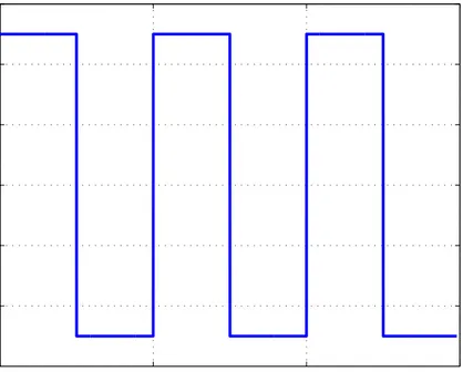
0 50 100 150 −6 −4 −2 0 2 4 6 Process Noise time (sec.) Noise Magnitude

Figure 3.1: Process Noise w(t)

Output is the position with an unknown signal and it is the signal to be estimated.

y(t) = p(t) + v(t) z(t) = p(t)

The disturbance w(t), initial value of state and ε are the leading effects on the movement of the vehicle. In order to see the maneuvers in the movement

w(t) is chosen as finite energy signal as in Figure 3.1 which leads the maneuvers

in Figure 3.3 which shows the vehicle behaviour in terms of its position in one dimension. Initial value of state and ε parameter are arbitrarily chosen as x(0) = h

0 0 0 iT

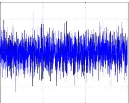
and ε = 2 respectively. Additionally, different values of ε will be illustrated. Also in all simulations band-limited white noise ˆv(t) is used as the measurement noise which is shown in Figure 3.2.

Our main objective throughout this work is to make an estimation of the state of a system with time delays. However it is aimed in this section to describe the

0 50 100 150 −15 −10 −5 0 5 10 15 Measurement Noise time (sec.) Noise Magnitude

Figure 3.2: Measurement Noise v(t)

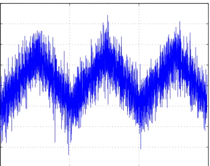
0 50 100 150 0 500 1000 1500 2000 2500 3000 3500 4000 4500 5000 Original Trajectory time (sec.) path

vehicle characteristics that will be used in simulations. That’s why the delay issue has never been mentioned. Following sections include modified versions of the dynamic system which is issued here. Main difference will be the delay that will appear somewhere in the system.

3.2

Illustrative Examples and Simulation

Re-sults

Many different variations of vehicle tracking problem are illustrated in this section to investigate the filter performance against different situations. Simulations were performed by the help of MATLAB-Simulink. First, we will see how the amount of delay affects the filter performance and try to find whether the filter has a limitation in terms of delay amount. Then the ε parameter will be changed in order to see how the different initial values of acceleration impact the filter performance. It will be shown that the existence of delay in state variable does not create difficulties for the solution.

In order to get comparable results of different situations all the simulations were performed with dynamic system mentioned in previous section changing the related parameter in each simulation. Moreover all the simulations are one-dimensional and can be easily extended to 2 or 3 one-dimensional cases.

3.2.1

Single Delay in Output

Delay in Output - Case 1

Consider the linear system defined in (2.1) and (2.2) with no delay in state and only one delay in output. In this case we have

˙x(t) = Ax(t) + Bw(t) (3.1)

y(t) = Cx(t − h) + Dv(t) (3.2)

In order to reach the error expression in Chapter 2, it is necessary to take the Laplace transforms of (3.1) and (3.2) which are given in (3.3) and (3.5).

X(s) = (sI − A)−1_{B + W (s) (3.3)}

Y (s) = CX(s)e−hs_{+ DV (s) (3.4)}

= C((sI − A)−1_{B + W (s)) + DV (s)}

We know that z(t) = Lx(t) will be estimated by a filter denoted by F (s) and

L = C which is assumed previously. Then

E(s) = Z(s) − ˆZ(s) = LX(s) − F (s)Y (s) (3.5) = LX(s) − F (s)(CX(s)e−hs_{+ DV (s))}

= CX(s) − F (s)e−hs_{CR(s)W (s) − F (s)DV (s)}

= (1 − F (s)e−hs)P0(s)W (s) − F (s)DWv(s) ˆV (s)

where R(s) = (sI − A)−1_{B, V (s) = W}

v(s) ˆV (s) and P0(s) = CR(s). Then the L2 induced norm is

γ = k(1 − F (s)e−hs)P0(s) − F (s)DWv(s)kH∞ (3.6)

Note that A, B, C and D matrices were given in Section 3.1.1: Delay in the output is equal to 0.4 (h = 0.4) and ε is taken as 2.

= h 1 0 0 i      s −1 0 0 s −1 0 0 s + 2      −1     0 0 1      (3.7) = 1 s2_{(s + 2)} DWv(s) = 1 (3.8)

According to the optimal filter solution in Chapter 2, filter equation is:

F (s) = Eγ(s)md(s) N−1 0 Fγ(s)L(s) 1 + e−0.4s_F γ(s)L(s)(1 + Eγ(s)) (3.9) Eγ(s) = ( 1 γ2P0(s)P0(−s) − 1) = − 1 + γ2_s4_(s2_{− 4)} γ2_s4_(s2_{− 4)}

with γopt= 1.1486. For the above numerical values Fγ(s) and L(s) are found as:

Fγ(s) = nFγ(s) dFγ(s) = s4− 4s2 0.8706s4_{+ 4.086s}3_{+ 6.108s}2_{+ 3.263s + 0.8566} L(s) = nL(s) dL(s) = − s2 _{+ 2.326s + 0.662} s2_{− 2.326s + 0.662}

After some operations desired filter turns into

F (s) = (e −0.4s_{− γ}2_s2_dF γ_nLdL 1 + γ2_s4_(s2_{− 4)} ) −1 = γ(1 + γe −0.4s_{− 1 − γ}2_s4_(s2_{− 4) − γ}2_s2_dF γdL_nL 1 + γ2_s4_(s2_{− 4)} ) −1 _(3.10) If s2_(s2_{− 4) + dF}

γ0 and −1 + L0 = −1 + dL_nL0₀ are used instead of γdFγ and L−1

respectively then the resulting filter turns into the form of

F (s) = γ R1(s)

1 + R1(s)R2(s)

(3.11) where R1(s) and R2(s) are Infinite Impulse Response (IIR) and Finite Impulse

the time interval [0 , 1]. For the above numerical values of the problem we have R1(s) = s 2_{+ 2.326s + 0.662} s2_{+ 2.368s + 0.7603} R2(s) = 0.8706e−0.4s s6_{− 4s}4 _{+ 0.758} + 10−2(0.0074s5− 0.09476s4+ 0.9289s3− 6.965s2+ 34.83s − 87.06) s6_{− 4s}4_{+ 0.758}

The signal namely the position of the vehicle to be estimated z(t) is given in Figure 3.3 of which maneuvered shape is provided by process noise w(t) in Figure 3.1.

While Figure 3.4 shows the difference between output and original trajectory (z(t) − y(t)), Figure 3.5 is the difference between the estimation and original trajectory (z(t) − ˆz(t)). Figure 3.4 is the error in the output of the system. It is

clearly shown the effect of time delay and this delayed information needs to be corrected. As a result, corrective effect of the filter is obviously seen in Figure 3.5.

Figure 3.5 shows that the filter successfuly eliminates the effect of time delay. Since the problem is not just a simple noise elimination problem, noise in Figure 3.2 still remains at the output of filter.

Delay in Output - Case 2

The only difference in this case according to Case 1 is the time delay which is used as h = 2 which leads γ to a greater value. γ = 2.4333 is found and Figure 3.7 is the estimation error of the filter which is designed to suppress the effect of time delay seen in output error in Figure 3.6. Resulting filter used in simulations is composed of following expressions which are placed into 3.11.

R1(s) =

s3 _{+ 4.309s}2 _{+ 5.246s + 1.255} s3 _{+ 4.814s}2 _{+ 7.234s + 3.213}

0 50 100 150 −10 −5 0 5 10 15 20 25 30 35 Error in output time (s) error

Figure 3.4: z(t) − y(t) for Case 1

0 50 100 150 −20 −15 −10 −5 0 5 10 15 20 Estimation Error time (s) error

0 50 100 150 −20 0 20 40 60 80 100 120 140 Error in output time (s) error

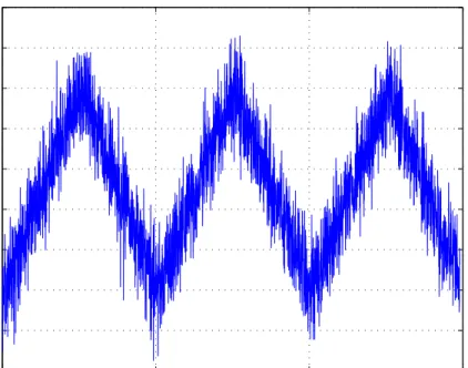
Figure 3.6: z(t) − y(t) for Case 2

R2(s) = 0.411e−2s s6 _{− 4s}4_{+ 0.1689} − 0.1908s 4_{− 0.6158s}3_{+ 0.6785s}2 _{− 0.5263s + 0.2165} s5 _{− 1.997s}4_{− 0.01061s}3_{+ 0.0212s}2_{− 0.04233s + 0.08456}

We have obtained similar effect as in Case 1. Greater time delay causes larger magnitude of error. However it can be said that the filter works successfully against time delay.

Delay in Output - Case 3

Let h = 6 be the only difference for this case as in Case 2, then the resulting filter expression is same with Case 1 and 2. Time delay has the largest value of these three cases so does γ which we have γ = 9.086. Optimal filter in 3.11 has

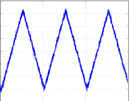
0 50 100 150 −50 −40 −30 −20 −10 0 10 20 30 40 Estimation Error time (s) error

Figure 3.7: Estimation Error (z(t) − ˆz(t)) for Case 2

the following expressions:

R1(s) = s3_{+ 4.171s}2_{+ 4.685s + 0.6858} s3 _{+ 5.846s}2 _{+ 11.36s + 7.341} R2(s) = 0.11e−6s s6_{− 4s}4_{+ 0.0121} − 1.04s4− 2.589s3+ 1.191s2− 0.375s + 0.06484 s5_{− 2s}4_{− 0.0007574s}3_{+ 0.001515s}2_{− 0.003s + 0.006}

Figure 3.8 and Figure 3.9 are the output error and estimation error respec-tively, namely z(t) − y(t) and z(t) − ˆz(t).

Above three cases show that noise characteristics in terms of the noise mag-nitude of the estimation error changes proportional to time delay and also to γ. Actually, the infinite frequency response of the filter creates this effect. Since

|F (j∞)| = γ as derived in (3.11), magnitude of noisy components of the

0 50 100 150 −50 0 50 100 150 200 250 300 350 400 Error in output time (s) error

Figure 3.8: z(t) − y(t) for Case 3

0 50 100 150 −150 −100 −50 0 50 100 150 Estimation Error time (s) error

0 50 100 150 −150 −100 −50 0 50 100 150 Disturbance in Output time (sec.) Magnitude

Figure 3.10: Measurement Noise associated with a High Pass Filter Delay in Output with High Pass Characteristics Disturbance - Case 4

In order to reduce the effect of the measurement error which were seen in esti-mation error in the above cases, we may consider using a weight Wv(s) which

generates v(t). Let h = 2 and DWv(s) = 10s+1_s+10 which shapes the measurement

noise in Figure 3.2 as in Figure 3.10. γ = 2.8245 is found for this case and derivation of the filter is same as the above filters.

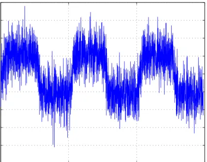
Figure 3.11 and Figure 3.12 are the output error and estimation error respec-tively. In this case the noise seen at the output is amplified relative to earlier cases however the filter succeeds suppressing the noise in partially in addition to eliminating the effect of time delay.

0 50 100 150 −150 −100 −50 0 50 100 150 200 250 Error in output time (s) error

Figure 3.11: z(t) − y(t) for Case 4

0 50 100 150 −50 −40 −30 −20 −10 0 10 20 30 40 50 Estimation Error time (s) error

0 50 100 150 −100 −80 −60 −40 −20 0 20 Estimation Error time (s) error

Figure 3.13: Estimation Error (z(t) − ˆz(t)) for the System with Actual Delay is

1

What happens if the actual delay is different than the delay used in filter design?

All the above filters were designed for exact value of delay. One can wonder what will happen if the actual delay is not exactly same as the delay that the filter is designed for. To illustrate this situation following simulations were performed.

Consider the problem in Case 2 which has 2 seconds time delay. However the delay in the system is taken different than 2. Figure 3.13 and Figure 3.14 show the cases where the time delays are 1 second and 3 seconds respectively.

From the figures it is clarified that the different delays in the system and that for design can take the results further than the desired ones. Actually the greater time difference between assumed (for what the filter is designed) and actual delays cause greater error. So it can be said that the actual time delay

0 50 100 150 −40 −20 0 20 40 60 80 100 Estimation Error time (s) error

Figure 3.14: Estimation Error (z(t) − ˆz(t)) for the System with Actual Delay is

3

has to be determined with maximum accuracy in order to get best performance from the filter.

Change in ε-parameter

ε-parameter which determines how much the initial value of the state impacts

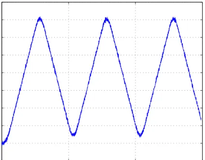
system dynamics is used as 2 in the above simulations. The next two simulations will show the capability of filter against smaller and larger ε’s. While Figure 3.15 and Figure 3.16 show the output and estimation errors when ε = 0.2, Figure 3.17 and Figure 3.18 are the output and estimation errors when ε = 10 respectively. In these simulations all the numeric values except than ε are same with the values in Case 4.

Small ε creates poles near to the imaginary axis in P0(s) than it seems that

small ε leads the output somewhat different than the original state. However the filter is able to track the original trajectory in both cases.

0 50 100 150 −200 0 200 400 600 800 1000 1200 Error in output time (s) error

Figure 3.15: z(t) − y(t) for the system with ε = 0.2

0 50 100 150 −150 −100 −50 0 50 100 150 Estimation Error time (s) error

0 50 100 150 −150 −100 −50 0 50 100 150 Error in output time (s) error

Figure 3.17: z(t) − y(t) for the system with ε = 10

0 50 100 150 −25 −20 −15 −10 −5 0 5 10 15 20 Estimation Error time (s) error

0 0.2 0.4 0.6 0.8 1 2 2.2 2.4 2.6 2.8 3 3.2 3.4 3.6 3.8 alpha₁ gamma 1 +gamma 2

Figure 3.19: γ1+ γ2 for Suboptimal Filter Approach

3.2.2

Multiple Delay in Output

Consider the dynamic system with two outputs with delay h1 = 0.4 and h2 = 2.

The solution method mentioned in Section 2.4.2 is applied onto this problem. Corresponding parameters α1 and α2 related with h1 and h2 are searched between

[0, 1] with D1Wv = 20s + 1 s + 5 D2Wv = 5s + 1 s + 0.8 in order to minimize γ1+ γ2.

Figure 3.19 is γ1 + γ2 versus α1 which shows that γ values corresponding to α1 = 0 and α2 = 1 are the optimum values to form the suboptimal filter.

In fact, there may be some other examples for different values of h1, h2, D1, D2 such that the optimal value of γ1+ γ2 is attained in the interval 0 < α < 1.

Figure 3.19 can be minimized anywhere which means γ1 and γ2 can take different

3.2.3

Delay in both State and Output

Simulations up to now are very similar in terms of delay characteristics other than the amount of delays. In this section we consider time delay in the state in addition to one in the output. We expect that state delay will clearly change the original trajectory. Therefore the change in state has a little effect on output but no more effort will be needed since it does not disturb the general structure mentioned and derived above. Case 4 of the previous section is repeated here by adding one delay to the state. So new structure of (2.1)and (2.2) are as in (3.12) and (3.13). ˙x(t) = A0x(t) + A1x(t − h1) + Bw(t) (3.12) y(t) = Cx(t − h2) + Dv(t) (3.13) Choose A0 = A1 =      0 1 0 0 0 1 0 0 −2     , h1 = 1, h2 = 2, DWv(s) = 10s + 1 s + 10

Then P0 changes accordingly: P0(s) =

(1 + e−2s₎2

s2_{(s + 2 + 2e}−2s₎ and γ = 4.4089 are found.

We approximate P0(s) using high order Pade approximation so that this approach

work. Remaining part of the solution is performed same with the previous ones. Resulting estimation error of the filter z(t) − ˆz(t) is shown in Figure 3.21 where

0 50 100 150 −150 −100 −50 0 50 100 150 200 250 300 350 Error in output time (s) error

Figure 3.20: z(t) − y(t) if the State has Time Delay in addition to that in Measurement 0 50 100 150 −80 −60 −40 −20 0 20 40 60 80 Estimation Error time (s) error

Figure 3.21: Estimation Error (z(t)−ˆz(t)) if the State has Time Delay in addition

3.3

Comparative Results

In this section the simulation results obtained with newly derived filter will be compared to ones from the literature. Since Kalman Filter is best known method for estimation purposes it will be illustrated first, then the method of Mirkin will be applied to the same vehicle tracking problem because we expect similar results to ours with his near optimal filter.

3.3.1

Kalman Filter Approach

Kalman Filter is the well known filtering method for Estimation applications. In order to see how it behaves in case of existence of delay in the system we will firstly discretize the continuous time linear system which is defined with (3.1) and (3.2).

˙x(t) = Ax(t) + Bw(t)

y(t) = Cx(t − h) + Dv(t)

Kalman Filter works with white process and measurement noise with zero mean Gaussian distribution. Since the process noise shown with the Figure 3.1 is a finite energy signal, it is needed to make simple modifications on this noise to use it as the process noise for Kalman filter.

Write w(t) as below:

w(t) = xw(t) + n1

˙xw(t) = n2

where xw(t) is a finite energy signal with zero derivative and noises n1 and n2

The dynamic equations defined by (3.1) and (3.2) turns into the below expres-sions: ˙˜x(t) = A˜x(t) + B ˜w(t) y(t) = C ˜x(t − h) + Dv(t) where ˜ x =   x xw   ˜w =   n1 n2   A =   A B 0 0   B =   B 0 0 I   C =h C 0 i .

Single Delay in Output Case is handled firstly to investigate and compare the performance of two methods. Let sampling time be Ts and h À Ts then

h = NTs. When the differential equation is solved x(t) is found as

˜

x(t) = eAt_{x(0) +˜}

Z _t

0

eA(t−τ )_{B ˜w(τ )dτ}

Writing this expression for x(tk+1) and x(tk) gives

˜ x((k + 1)Ts)) = eATsx(kT˜ s) + Z _(k+1)Ts kTs eA((k+1)Ts−τ )B ˜w(τ )dτ use ˜w(τ ) ≈ ˜w(kTs) on τ ∈ [kTs (k + 1)Ts] then ˜ x(k + 1) = Adx(k) + B˜ dw(k)˜

where Ad= eATs and Bd=

R_Ts

0 eAτBdτ

(3.1) and (3.2) can further be written in discrete time as ˜

x(k + 1) = Adx(k) + B˜ dw(k)˜

It is better to write in augmented state with below relations ˜ x1(k) = ˜x(k) ˜ x2(k) = ˜x(k − 1) ˜ x3(k) = ˜x(k − 2) ... ˜ xN +1(k) = ˜x(k − N) ¯ x(k) =          ˜ x1(k) ˜ x2(k) ... ˜ xN +1(k)          =⇒ x(k + 1) =¯          ˜ x1(k + 1) = ˜x(k + 1) ˜ x2(k + 1) = ˜x1(k) ... ˜ xN +1(k + 1) = ˜xN(k)          ¯ Ad=             Ad 0 . . . 0 I 0 . . . 0 0 I 0 . . . 0 ... ... ... ... ... 0 . . . 0 I 0             ¯ Bd=          Bd 0 ... 0          ¯ Cd= h 0 . . . 0 C i ¯ Dd = D

Augmented system equations are expressed as: ¯

x(k + 1) = ¯Adx(k) + ¯¯ Bdw(k)¯

y(k) = ¯Cdx(k) + ¯¯ Ddv(k)¯

w(k) and v(k) are process and measurement noises assumed to be zero mean

Gaussian distribution with covariances Qk and Rk.

¯

w(k) ∼ N(0, Qk)

¯

v(k) ∼ N(0, Rk)

Since we do not have a restriction in terms of noise characteristics in H∞solution

we do not use the exactly same noise used in H∞ filtering solution. Then Qk =

Numerical Example

Case 1 of Section 3.2.1 is repeated in order to compare the performance of two filters. Firstly it is needed to find new system dynamics. Sampling time Ts = 0.05

seconds and time delay h = 0.4 which results N = 8 are used. After necessary calculations Ad and Bd are found as;

Ad =          1 0.05 0.0012 2· 10−5 0 1 0.0476 0.0012 0 0 0.9048 0.0476 0 0 0 1          Bd = 1 8          2T2 s − 2Ts− e−2Ts + 1 2₃Ts3− Ts2+ Ts+1₂e−2Ts − 1₂ 2(2Ts+ e−2Ts− 1) 2Ts2− 2Ts− e−2Ts + 1 4(1 − e−2Ts_{) 2(2T} s+ e−2Ts − 1) 0 8Ts          = 10−2          2· 10−3 _{2· 10}−5 0.12 2· 10−3 4.7 0.12 0 0.05         

Different Kalman filter updates are applied to each 25 seconds period of original trajectory where the process noise w(t) of H∞ filter problem which is

shown by Figure 3.1 is either 5 or −5. The first 25 seconds period is handled here and error of H∞ filter and Kalman filter in this interval are shown by Figure

3.22 and by Figure 3.23 respectively. Kalman Filter updates begin with initial state

h

0 0 0 5 iT

.

Kalman Filter error according to Figure 3.22 seems better than H∞ filter

result. However Kalman filter needs to know exact time delay to form the state space representation in discrete time and also time delay must be an integer multiple of sampling time. Otherwise H∞ filtering method does not regard such

0 5 10 15 20 25 −0.05 0 0.05 0.1 0.15 0.2 0.25 0.3 time (s) error

Estimation Error (Kalman Filter)

Figure 3.22: Estimation Error (z(t) − ˆz(t)) for the Kalman Filter with initial

state with process noise information

restrictions on time delay. In addition to this, the main difference between two methods is the statics of process noise. While H∞filtering method works without

any information about process noise, Kalman filter takes it into account as seen in above derivations and as the last element of initial state. Figure 3.24 is the Kalman filter error in case that the initial state is

h

0 0 0 0 iT

in the interval

t ∈ [0, 25] which means there is no information about the signal, w(t), of Figure

3.1. Figure 3.25 shows Kalman Filter error in complete time duration where process noise, w(t), is 5 and −5 consecutively. Thus, when there is no initial condition information H∞ works better.

3.3.2

Mirkin’s H

Suboptimal Filter Approach

Extraction of dead-time estimators from parametrization of all delay-free estima-tors is proposed in Mirkin’s method [17]. This approach enables a straightforward reduction of various dead-time problems to a special one-block distance problem.

0 5 10 15 20 25 −10 −5 0 5 10 15 20 Estimation Error time (s) error

Figure 3.23: Estimation error (z(t) − ˆz(t)) for t ∈ [0, 25] of Case 1 in Section

3.2.1

Also near optimal H∞ estimator is a generalized Smith predictor. In Figure 3.26

it is shown that delay is augmented to the plant P resulting in the design of an unconstrained estimator for infinite dimensional system. Classical Nehari prob-lem is solved during solution process of this probprob-lem. Solvability conditions are applied on the problem to find Kh which is in the form of the Figure 3.27.

Numerical Examples

Case 1 in Section 3.2.1

Solution of this approach gets a central suboptimal filter. Basically the filter elements Ga and Ja are found as following:

Ja(s) = 3.31s2_{+ 7.843s + 2.483} s3_{+ 4.826s}2_{+ 6.85s + 2.483} Ga(s) = e−0.4s s6_{− 4s}4_{+ 0.5102}

0 5 10 15 20 25 0 10 20 30 40 50 60 70 80 time (s) error

Estimation error (Kalman Filter)

Figure 3.24: Estimation Error (z(t)− ˆz(t)) for the Kalman Filter without process

noise information

− 4.42 10

−5_s5_{− 5.56 10}−4_s4 _{+ 5.44 10}−3_s3_{− 4.08 10}−2_s2_{+ 0.2041s − 0.5102} s6 _{− 4s}4 _{+ 0.5102}

Then the resulting filter is

Kh =

Ja(s)

1 − Ja(s)Ga(s)

Suboptimal γ which is satisfied by suboptimal filter is found as ∼ 1.4 which is larger than optimal γ which is 1.1486.

Figure 3.28 is the estimation error of the optimal and central suboptimal filters together where the darker one with smaller amplitude is the result of Mirkin’s method. It is seen that central suboptimal filter reduces the effect of noise by the help of low pass filter characteristics. This is due to the gain of the optimal filter at s = +∞, i.e., in Case 1 to 2 we have F (∞) = γ, which means that the high frequency component of the noise is amplified/attenuated by a factor of γ. Whereas the central suboptimal filter of [17] is always strictly

0 50 100 150 −150 −100 −50 0 50 100 150 time (s) error

Estimation Error (Kalman Filter)

Figure 3.25: Estimation Error (z(t)− ˆz(t)) for the Kalman Filter without process

noise information

proper, hence high frequency noise is always filtered. However avarage value of estimation error of suboptimal filter is larger than that of the optimal filter where average error values of optimal filter and suboptimal values are 2.611 and 4.076 respectively in the time period [0, 25] and −2.176 and −3.77 respectively in the time period [26, 50].

Case 4 in Section 3.2.1

Necessary calculations have been performed as in above example to compare with the another designed filter. Suboptimal γ ≈ 3 which is greater than optimal

γ which has been found as 2.8245. The expressions that form the estimator are

found as below: Ja(s) = − 21.16s3_{+ 50.68s}2_{+ 17.4s + 1.254} s4_{+ 10.32s}3_{+ 26.56s}2_{+ 24.77s + 12.55} Ga(s) = 0.051(s + 10)e−2s s7_{+ 0.1s}6_{− 4s}5_{− 0.4s}4_{+ 0.5102s + 0.05102}