Boundary control of a Timoshenko beam attached to a rigid body: planar motion

Boundary control of a Timoshenko beam attached to a rigid body:

planar motion

OMER MORGOLt

A flexible spacecraft modelled as a rigid body which rotates in an inertial space is considered; a light flexible beam is clamped to the rigid body at one end and free at the other end. The equations of motion are obtained by using the geometrically exact beam model for the flexible beam, and it is then shown that under planar motion assumption, linearization of this model yieldsthe Timoshenko beam model. Itis shown that suitable boundary controls applied to the free end of the beam and a control torque applied to the rigid body stabilize the system. The proof is obtained by using a Lyapunov functional based on the energy of the system.

1. Introduction

Many mechanical systems, such as spacecraft with flexible appendages or robot arms with flexible links, can be modelled as coupled elastic and rigid parts. Many future space applications, such as the space station, rely on lightweight materials and high performance control systems for high precision pointing, tracking, etc., and to achieve high precision demands for such systems, one has to take the dynamic effect of flexible parts into account. Thus, over the last decade there has been a growing interest in obtaining new methods for the design, analysis and control of systems which have flexible parts. An excellent review of research in this area can be found in the work of Balas (1982).

The overall equations of motion of a system which has coupled elastic and rigid parts are usually a set of coupled non-linear ordinary and partial differential equations with appropriate boundary conditions. These equations can be obtained by using standard methods of mechanics (see for example Goldstein 1980). How-ever, it should be noted that, although the mechanics of rigid bodies are well understood, this is not so for flexible bodies. There are many flexible body models and choosing one is not a trivial task (see e.g. Russell 1986).

In the analysis of such coupled rigid and flexible body systems, particularly in engineering applications the commonly used approach is to express the solutions (e.g. the displacements caused by elastic motion) as an infinite sum in terms of the eigenfunctions corresponding to the relevant (linear) partial differential equation, and then to consider only finitely many terms in this sum, see Meirovitch (1967), Balas (1982). This approach is called 'modal' analysis and reduces the original set of equations, which are coupled non-linear ordinary and partial differential equa-tions, to a finite, although often very large, set of coupled non-linear ordinary differential equations. However, having established a control law for this reduced set of equations does not always guarantee that the same law will work on the original set of equations (e.g. one might encounter the so-called 'spillover'

Received 16 October 1989. Revised 25 December 1990.

[Department of Electrical and Electronics Engineering, Bilkent University, 06533, Bilkent, Ankara, Turkey.

764

O.

Morgiil

problems-see Balas 1978). Also note that the actual number of modes of an elastic system, in theory, is infinite and the number of modes that should be retained is not known a priori.

The stability of systems which have elastic parts, particularly flexible space structures, has been studied in the past. Recently, Biswas (1986) used a Lyapunov type approach which uses the total energy of a flexible structure as a Lyapunov function to prove the stability of the system under appropriate control forces and torques applied to the flexible structure. The proposed control law contains distributed forces applied to the flexible structure (i.e. forces that are distributed over the flexible structure), which are proportional to the deflection velocities. Implementations of such control laws might not be easy or practical.

In recent years, the boundary control of flexible systems (i.e. controls applied to the boundaries of the flexible parts as opposed to controls distributed over the flexible parts), has become an important research area. Quinn and Russell (1978) established the uniform stabilization of the one-dimensional wave equation with boundary control, and later Chen (1979) obtained similar results for the wave equation in arbitrary space dimensions. More recently, Chen et al. (1987 a, b) established the uniform stabilization of the Euler-Bernoulli beam with boundary control, and Kim and Renardy (1987) obtained similar results for the Timoshenko beam. In particular, Chen (1987 a) proved that in a cantilever beam, a single actuator applied at the free end of the beam is sufficient to stabilize the beam deflections uniformly and exponentially; and Delfour et al. (1986) investigated the case where the actuator is 'concentrated' on an area, as opposed to a single point. Recently, boundary control techniques have been applied to the stabilization of a flexible spacecraft, modelled as an Euler-Bernoulli beam attached to a rigid body, performing planar motion (Desoer and Morgiil 1988), and three-dimensional motion (Morgiil 1990).

In this paper, the motion of a flexible beam clamped to a rigid body at one end and free at the other end is studied. It is assumed that the mass of the rigid body is much larger than the mass of the flexible beam; hence it can be taken that the centre of mass of the rigid body is also the centre of mass of the whole system. It

is also assumed that the centre of mass of the rigid body is fixed in an inertial frame. This assumption can be justified if one considers a satellite in a geosyn-chronous orbit, since in this case, neglecting the rotation of the Earth, the centre of mass of the satellite is fixed with respect to the Earth.

The so-called geometrically exact beam model for the flexible beam has been used (for details see Simo 1985, Vu-Quoc 1986). In §2, a basic review is given of this beam model. As an example, the equations of motion for the planar motion of a flexible beam modelled as a geometrically exact beam are obtained, and it is shown that linearization of the equations of motion for this particular case leads to the well-known Timoshenko beam equations (see Meirovitch 1967). Although the Timoshenko beam equations are more complex than those of the Euler-Bernoulli or Rayleigh beam equations, it is known that for large motions the results from the Timoshenko beam equations are in remarkably good agreement with those ob-tained from the exact theory of elasticity (see Bakr and Shabana 1987 and the references therein).

In §3 we introduce the basic rigid-body flexible-beam configuration studied in this paper, and using the geometrically exact beam model we obtain the equations of motion. We then define the rest state of this system and pose a stabilization

problem: i.e., if the system is perturbed from the rest state, how may one find appropriate control laws that drive the system back to that rest state. We then propose a control law that consists the appropriate boundary control force and moments applied at the free end of the beam and a control torque applied to the rigid body.

In § 4, it is first shown that the proposed control law stabilizes the system in the sense that the 'energy' of the system becomes a non-increasing function of time. Then, assuming planar motion, linearize the equations of motion of the beam, which results in the equations of motion for a Timoshenko beam, clamped to a rigid body at one end and free at the other end. We show that the proposed control law asymptotically stabilizes the system; more precisely, we prove that the 'energy' of this system decays as D( 1ft) for large t.

In § 5 we first give an existence and uniqueness result: then we prove that the 'energy' of the system decays exponentially to zero.

In § 6, we present some simulation results and finally we give some concluding remarks.

2. Review of the geometrically exact beam model Kinematics

Let the quadruople N= (e, e2 , eJ ) denote an inertial frame with the origin 0

and with the orthonormal dextral (i.e. right-handed) basis vectorse" e2 ,eJ .Let the

flexible beam be initially straight along the e2axis; we refer to this configuration as

the reference configuration of the beam. We assume that one end of the beam is clamped to a rigid base fixed in N and the other end is free.

We associate the beam two geometrical objects: a set of planar cross-sections and a curve of centroids which pass through the centre of mass of each cross-section. Hence, in the reference configuration, the curve of centroids is a line along the direction of the e2axis. Initially, we take the cross-sections perpendicular to this

line. We assume that, throughout the motion, the planar sections remain planar. We also assume that the beam is homogeneous with uniform cross-sections.

Let P be a typical beam element whose distance from 0 in the reference configuation is x. Let L be the length of the beam in the reference configuration, hence we have 0,,; x ,,;L. We take x as a coordinate along the curve of centroids. Letrex, t)

=

0 P be the position vector of P. Hence, initially we have rB(x,0)

=

xe_{2 .}

Let C, denote the cross-section at x and let P also denote its centre at the curve of centroids. Let the quadruple (P, d, d2 ,d3 ) denote a frame with its origin at P

and with orthonormal dextral vectors d, d2 ,d, such that the axes d, d, lie in the

cross-section C; and the axis d2 is normal to C, at all times. We denote this as the

frame of directors at x.

Let A(x, I) denote the orthogonal transformation matrix between the basis of the inertial frame e" e2 ,e3 and the basis of the frame of directors d, d2 ,d3 ; more

precisely, we have for all 0,,; x ,,;L,1 ;" 0:

3

dj =

2:

Aij(X't)ej , j = 1,2,3 i=I

where Aijdenotes the (i,j)th component of the matrix A. Initially choose

(I)

766

O.

Morgul

Upon differentiating A(x, I) with respect to x and 1we obtain

a

a

-a

A(x, I)= W(x, I)A(x, I)

-a

A(x, I)= Q(x, I)A(x, I)

1 x (3)

where, for all 1~0, 0,;;;x ,;;; L, W(x, I) and Q(x, t) are 3 x 3 skew-symmetric

matrices. Let the parameterization of Wand Q be given by

( 4)

where, for the sake of simplicity, we suppress the dependency on x and I.

We define the axial vectors wand 1I) associated with the skew-symmetric matrices Wand Q as follows:

3 w:=

L

w.d., i=l 3 lI)'=

I

oi.d, i= I (5) ( 6) (7) (9)

Following Simo (1985), we define the pull-back K of1I)by A, which is a measure of the curvature of the curve of centroids, and the strain measure F, as follows:

Tar

f,=A _{- - ez}

ox

where the superscript T denotes the transpose.

We note the following relation between K and 1I) (see Simo 1985):

aK= AT all)

al

ax

We define the contact force n(x,I) and the contact moment m(x, I) as follows. Consider a beam cross-section C, at x. The effect of the material which lies on the (x, L) segment of the beam on the material which lies on the [0,

xl

side of the beam is equivalent to a force and to a moment applied to the cross-section C" these are called the contact force and the contact moment, respectively (see Antman 1972).

Dynamics

We assume that the internal energy 'I' of the beam is a function ofx, K and I'

where the last two vectors are defined in (6). The equations of motion of a geometrically exact beam described above, together with the boundary conditions and the constitutive relations are given as follows, for all 0,;;;x ,;;;L,1~0:

an

aZr

ax

+

fl = P

al

z (8)

am

ar

--a +--a

xn+1=!Bw+WX!BW x x

a

1/1 n = A

-ar'

r(O,I) = 0, n(L,I)= f(l), A(O,I) =! m(L,I)= g(l) ( 10) (II) ( 12)

where ii and

m

are the applied force and moment per unit length, respectively, P

is the mass per unit length of the beam, [B is the inertia tensor of the beam cross-sections relative to the inertial frame N, and f(t) and g(t) are the boundary control force and moment applied to the free end of the beam respectively.

Note that (8) is the balance of forces, (9) is the balance of moments at the beam cross-sections, (10) gives the constitutive relations, and (II) and (12) give the boundary conditions at the clamped and free ends, respectively.

Special case: planar motion of a linear inextensible beam

As an example, we consider the planar motion of the geometrically exact beam described above. We assume that the motion takes place in the plane spanned by the inertial axes ez and e3 for all t;;'0 and that we have d,(x, t)

=

e" for all

o

~x ~L, t ;;._{O. Let ¢ denote the angle between the axes e z and d z, measured as} the angle swept when the former axis is rotated around the axise, until its direction coincides with the direction of d z. Hence, the rotation matrix A takes the following form: [ I 0 A.= 0 cos¢

o

cos ¢ ( 13)

therefore the axial vectors w, roand the vector K become

Let the position vector r(x, t) = 0P be parametrized as follows: r(x, t)

.=

_xez

+

u(x, t)e3

( 14)

( 15) where u(x, t)denotes the beam displacement along the axis e3 . Here we assume that

the beam displacement along the axis

_{e z}

is identically zero, i.e. the beam is inextensible.

The contact force n, the contact moment m and the strain measure

r

take the following form:

(16) Using (6), assuming that u and ¢ are small and neglecting higher order terms, we obtain

( 17) As is often assumed in practice, we take the following quadratic form for the internal energy:

(18) where K = iJ¢liJx; GA is called the shear stiffness (along the axis d_{3 ) ;} and EI is called the principal bending stiffness (relative to the axis d.) (see Meirovitch 1967).

768

o.

Morgii/

Using (18) in (10), and then in (8), (9), and neglecting the axial motion, ii, m,

the equations of motion (8), (9) and the boundary conditions (II), (12) now become, for all I ~0, 0<x <L:

GA

(a

2u

_ a</J)

= p

a

2u

ax2

ax

bt? (19)

a

2r/J

(au

)

a

2r/J

EI

ax 2

+

GA

ax -

r/J = Ie

al2

(20) u(O, I) =0, r/J(O,I)=O (21) GA

(u.(L,

I)

-r/J(L,

I» =/(1), EI

r/J.(L,

I) =g(l) (22) where we take f(l) =/(1)83,9(1) =g(l)eJ ; also note that a variable sub-index

denotes partial differentiation with respect to the variable, e.g.

u.

=

auf ax,

etc. We note that (19) and (20) are the equations of motion for a Timoshenko beam (see Meirovitch 1967).

3. Equations of motion of flexible spacecraft

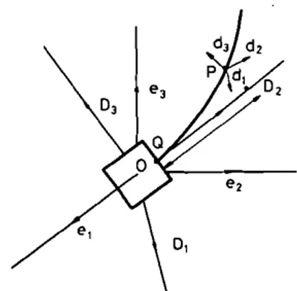
Consider the following configuration: Fig. I shows the rigid body (drawn as a square) and the beam; P is a point on the beam:

In Fig. I, the quadruple (0,e.,_{8 2, 8 3)} denotes a dextral orthonormal inertial frame, which will be referred to as N, the quadruple (0, OJ, O_{2 ,} 0_{3 )} denotes a dextral orthonormal frame fixed in the rigid body, which will be referred as B, where 0 is also the centre of mass of the rigid body and OJ, O_{2 ,} 03are along the

principle axes of inertia of the rigid body. The beam is clamped to the rigid body at the point Q at one end along the O₂ axis and is free at the other end. Let L be the length of the beam. We assume that the mass of the rigid body is much larger than the mass of the beam, so that the centre of mass of the rigid body is approximately the centre of mass of the whole configuration. Hence, we assume that the point 0 is fixed in the inertial space throughout the motion of the whole configuration. We also assume that the beam is inextensible (i.e. no deformation along the axis O_{2 ) ,} and homogeneous with uniform cross-section.

The beam is initially straight along the O2 axis. Let P be a point on the curve

of centroids whose distance from Qin the un deformed configuration isx (i.e. when

the beam is straight along the O2axis), let the quadruple (P,d., d2 ,d3 ) denote the

frame of the directors located at P, where d, d2 ,d, are the directors at x. Let

r(x, t)

=

OP be the position vector of P.

(23) (26) (24) (25) (27) (28) Let, I\(x, t) be the orthogonal transformation between the body frame and the frame of directors. Then, neglecting gravitation and surface loads and assuming that the centre of mass of the rigid body is fixed in the inertial frame N, the equations for flexible spacecraft are given by, for all t ;;;, 0,

°

<x < L:

an

=

(02

r )

ax p

ot

2 _N

am

or

(O(W

+

(J)R»)

7);

+

ax x n

=

IB at B

+

(w

+

(J)R) x IB(w

+

(J)R)

IRooR

+

(J)R X IR(J)R= r(O, I) x n(O, I)

+

m(O, I)

+

Nc(t)

olj; olj;

n = l \ - m = l \

-or'

OK

r(O,t)

=

00, 1\(0, t)

=

I

n(L, I)= f(I), m(L,t) = g(t)

where n(x,I) and m(x,t) are the contact force and the contact moment of the beam, respectively;(o( . ) /OI)N denotes that the time differentiation is taken in the frame N; pis the mass per unit length of the beam;IB is the inertia tensor of beam

cross-sections, which is a constant matrix by assumption; (J)R is the angular velocity

of the rigid body in the inertial frame N; IR is the inertia tensor of the rigid body,

which is a constant diagonal matrix by assumption; Nc(t) is the control torque applied to the rigid body; 'I'(r,K) is the internal energy (i.e. potential energy) per unit length of the beam, which at the moment need not be a quadratic function of its arguments; and f(t) and g(t) are the boundary control force and moment, respectively, both applied at the free end of the beam. Also note that the time derivation between different frames are related as follows (see Goldstein 1980):

(r')N = (r')B

+

(J)R X r (29)

Equations(23) and (24) state the balance of forces and the balance of moments at the beam cross-sections, respectively; (25) is the rigid body angular momentum equation; (26) is the constitutive equation of the beam; and (27) and (28) give the boundary conditions at the clamped end and at the free end, respectively (for details, see Morgiil 1989).

We define the rest state of the system given by (23)-(28) as follows:

(J)R = 0

or

ax = O2 , x E[0,L) (30) (31 ) I\(x)

=

I, x E[0,L) (32)

Itis easy to see that (30) holds for all t EIl\l+ if and only if the rigid body does not spin in the inertial frame N.

Let the curve of centroids be represented by

770

O.

Morgiil

and, by (27), II,(0, t) = 112(0,t) = 113(0,t) =

°

for all 1 ;;.0. Then (31) holds for all

t E IR+ if and only if the beam displacements _11,,112,113are identically zero. If (31) holds for all t E IR+, then the beam deflections II" _{112 , 113}do not depend

on time, hence by the first boundary condition in (27) they are identically zero on [0, L] x IR+. Conversely, if III> _{112, l/3} are identically zero on [0,L] x IR+, then (31)

trivially follows from (33).

Also note that (32) holds if and only if the strain measure K defined in (7) is identically zero on [0,L] x IR+. If (31) holds, then the second equation in (3) implies that the skew-symmetric matrix

!lex,

t) is identically zero on [0,L] x IR+, which then implies that the corresponding axial vector wand hence the strain measureK are all identically zero on [0,L] x IR+. Conversely, ifK is identically zero on [0, L] x IR+, then so is the axial vector wand the corresponding skew-symmetric matrix !l. Then (3) implies that A does not depend on x; hence by using boundary condition (5), we obtain(32). Furthermore, if(31) holds, (32) implies that the other strain measure

r

defined in (6) is also identically zero on [0,L] x IR+.

Stabilization problem

The stabilization problem is stated as follows: let the system given by(23)-(28) be disturbed from the rest state given by (30)-(32); find appropriate control laws Nc(t),f(t), get) that drive the system back to the rest state. 0 Natural control law

This control law applies a force n(L,t) and a torque m(L,t) at the free end of the beam and a torque Nc(t)to the rigid body. They are specified as follows: choose 3 x 3 symmetric positive definite matrices K, L, M (which can all be chosen diagonal); then for all I;;'0 the 'natural control law' requires that

n(L,t)

=

-L(r,(L, t»B m(L,I) = - Mw(L, t) Nc(t)

= -

r(L, t)

x

n(L,t) - m(L,t) - KWR (34) (35) (36) (37) This control law is 'natural' in the sense that it enables us to use the total energy of the system as a Lyapunov function to study its stability. 0 4. Stability results for the natural control law

Consider the system given by (23) -(26) together with the control law (34)-(36). To study the stability of this system, we define the energy of the system as follows for all 1 ;;.0:

E(t) =

!<WR,

IRw

R)

+~

r

p<r"r,)dx

+~

r

«w

R

+

w), IB(wR

+

w»dx

+

~

r

'P(r,K)dx

where

<.,.)

denotes the standard inner-product in 1R3

, and r, is the abbreviation

for (r,(x, I»N' The first term in (37) represents the rotational kinetic energy of the rigid body, the second term represents the kinetic energy of the beam in the inertial

frame N, the third term represents the rotational kinetic energy of the beam cross-sections and the last term represents the potential energy of the beam.

Proposition

Consider the system given by(23)-(28) and (34)-(36), which will be called the system Y. Then the energy £(1)defined in (37) is a non-increasing function of time

along the solutions of the system Y. 0

(39) (38)

(40)

(41) Proof

Differentiating (37) with respect to time t, we obtain

~~

= \ OOR,

:r

(IROOR) )

+r

p(r" fIC

>

dx

+r \

(OOR

+

w),

:r

[IB(ooR

+

W)])dx

+r\~,~)~+r\:,:)~

=(OOR' IRw R+OOR x IRooR

>

+

f-

«f')B

+

OOR X r, nx

>

dx

+

11.

\(OOR

+

W),IB

:t

(OOR

+

W)B

+

(OOR

+

w) X IB(ooR

+

W»)dx

+r\~;,~)~+r\~:,:)~

where in the second equation we use (23) and (29).

Using integration by parts, we calculate various integrals in (38) as follows:

1

o

1.

«r')B,nx)dx=«r')B(L,t),n(L,t»-

11.

0 «f')B,n>dx

f"

(OOR x r, n,) dx = \ OOR,

11.

r Xn,dX)= (OOR'

ru;

t) x n(L,

.»

- \ OOR,

r

r; X ndX)

1= \(OOR

+

w), IB

:t

(OOR

+

W)B

+

(OOR

+

w) X IB(ooR

+

w) ) dx

=

r

(OOR

+

w), rn,

+

r; X n)dx by(24)

=

r

(W,m,)dx+\OOR'

r

m,dx)

+

f-

(w,

r.

x n)dx

+ \

OOR,

11.

r, x ndX) = (w(L, t), m(L, t» - (w(O, t),m(O,t»

-r

(WI'm)dx

+

(OOR,m(L, t) - m(O,t»

+

1'-

(w x r, n)dx

+ \

OOR,

l

L

772

o.

Morgiil Using (39)-(41), we obtain

dE

dt = (wR,IRwR X IRw R

+

r(L, t)

x

n(L, t) - r(O,t) x n(O,t)

+

m(L, I) - m(O, I»

+«r')B(L, I), n(L, I»

+

(w(L, I), m(L, I» - (w(O, I), m(O, r]

-r

«rx,)B - w x rx ' n)dx -

r

(w

x ,m)dx

+

r

(~~,~~)dX+

r

(~:,~;)dX

Differentiating (7) with respect to time 1 and noting that the internal energy 'I'

of the beam is invariant under rigid body motions (i.e., 'I' measured in the body frame B is equal to 'I' measured in the inertial frame N-for details see, for example, Marsden 1983),we obtain

(a r ) (a T) ar I\.T ( a 2r ) T ar I\.T ( a2r ) - - -I\.

-+

- -

--I\.

w-+

-al B- al ax al ax B- ax al ax B

=

I\.T[(rx')B - w x rxJ (43)

where, in the second equation, we have used (3) and the skew-symmetry of W. Then, using the definition of the axial vector w associated with W,we obtain (43).

Using (8), (43), (25) and (26) in (42), we obtain

dE

r

L

.

dl

=

(wR,r(L,t) xn(L,I) +m(L,I)

+

Nc(t»-Jo «rx,)B-wxrx,n)dx

r

L

r

L

r

L

- Jo (w"m)dx

+

Jo (I\.Tn,I\.T[(rx,)B -w x rx])dx+ Jo (I\.Tm,I\.Tw,)dx +«r')B(L, I), n(L, r)

+

(w(L, t), m(L, I» - (w(O,z),m(O, I»

Since I\. is an orthogonal matrix, integral terms cancel each other. Also, by the boundary conditions (27), upon differentiating with respect to time t, at the clamped end we have:

(r,(O,t»)B=O, W(O,I) =0, I~O (45)

Using (44) and the control law (34)-(36) in (44), we obtain dE

dl

=

-(wR, KWR) - «r,(L, I»B, L(r,(L, t»B) - (w(L, r), Mw(L, t» (46) Since, by choice the matrices K,L,M are positive definite, it follows from (46) that the energy E(t) defined in (37) is a non-increasing function of time. 0

Remark I

In the derivation of (46) we have used the non-linear equations (23)-(28) without any linearization. Furthermore, we have imposed no restrictions on the internal energy 'I' of the beam, other than the assumptions that it depends on the strain measures rand K, and that it is invariant under rigid body motions, which

p. 194). From this assumption it follows that the rate of change of the internal energy 'I'as observed in the inertial frame N and as observed in the body frame B must be the same, since these two frames differ only by a rotation which does not

depend on the spatial coordinate x. 0

To prove that the solutions of(23) -(28) with the control law (34) -(36)decay to the rest state defined by (30) -( 32), we need to parametrize the orthogonal transformation matrix A and specify the form of the internal energy function '1'.

In what follows we assume that the whole motion takes place in a plane whose unit normal is the inertial axis e,. More precisely, we consider the configuration given in Fig. I with the following assumptions.

Assumptions

(a) The axes e" 0" d, coincide at all times and the rigid body may rotate only about the axis e,.

(b) The whole motion of the beam takes place in the plane spanned by the axes

e2 , 9 3 ·

(c) The axial deflection (i.e. along the O2axis) and the torsion (i.e. the rotation

of the beam cross-sections about O2 axis) are negligible.

(d) The internal energy 'I' is a quadratic function of its variables, see (18). 0 The orthogonal transformation matrix A between the body frame N and the frame of directors now admits representation given by (13), therefore the axial vectors W, 00, K can be given by (14).

Let the position vector r=

a

P be parametrized as follows:

r(x,I)=(b+x)02+UO) (47)

where b,=

1001

and u is the beam displacement along 0).

With these assumptions and neglecting the higher order terms, the relevant component form of equations (23)-(28) now reduce to (cf. (19)-(22))

GA (un -

</IJ

=

pUtt

+

pO(b

+

x) - p02U (48)

EI

</In

+

GA(u, -

</I)

= IB(</Itt

+

0) (49)

IR

O'

=

bGA [uAO, I) - </1(0,I)]

+

EI</lAO, I)

+

Nc(t) (50)

u(O,I) =0, </1(0,1)=0, 1;;;,0 (51) where b

=

1001,

</I

is the angle between the axes d2 and O2 , and (} is the angle of

rotation of the rigid body about the axis e,; hence we have lOR

=

00"

I_B is the

principal moment of inertia of the beam cross-sections about the axis d, and I_R is the principal moment of inertia of the rigid body about the axis 0,.

The component form of the natural control law (34)-(36) now becomes GA [uAL, I) - </I«L,I)] + rxu,(L, I) =

°

(52)

EI</IAL, I)

+

P</I,(L,I)

=

°

(53)

Nc(t) = -(b+ L) GA [uAL, I) - </I(L,I)] - EI</IAL, I) - kO (54) where k> 0, rx >0, and

P

>

°

are arbitrary positive numbers.

774

O.

Morgiil The total energy £(1) given by (37), now becomes

£(1) =

4/

RIF

+ 4

r

p<r" r,

>

dx

+ 4

r

IB(4),

+

8)2dx

+4

r

GA(u, - 4»2dx

+4

r

EI4>;dx

and the rate of change of£(1) given by (46) now reduces to d£

dI

= -k02 - ct.U~(L, I) - f34>~(L,I) (55) (56) Theorem I

Consider the system given by (48)-(51) together with the control law (52)-(54). Then there exists aT;. 0 such that for 1 ;.T, the energy £(1) given by (37)

decays as O( 1/1). 0

Remark 2

Equations (48)-( 51) are the component forms of equations (23) -(28) under the assumptions(a)-(d) stated after (46). As a result of these assumptions, (48)-(51) represent the equations of motion for the planar motion of a rigid body whose centre of mass is fixed in an inertial frame, with a beam modelled as a Timoshenko

beam clamped to it. 0

Remark 3

If we use the conclusion of Theorem I, (55) and (56), then we see that the solutions of (48) -( 51) tend to the rest state defined by (30) -( 32) as I ->CIJ. 0

Proof of Theorem I

We define the following function V(I):

V(I)

=

2(I - 8)1£(1)

+

2

r

px(u,

+

8(b

+

x))u, dx

+

2

r

I_Bx4>.A4>,

+

8)dx

+,)

r

IBrjJ(4),

+

8)dx -,)

r

pu[u,

+

8(b

+

x)] dx (57)

where 8 E(0, I) and ,)>0 are constants yet to be determined.

To prove the theorem, first show that there exists a constant C>0 such that the following estimate holds for all I ;.0:

[2( I - 8)1 - C]£(I) ,,;V(I) ,,;[2( I - 8)1

+

ej£(I)

then we prove that there exists a T_{1 ; .}0 such that

(58)

Combining (58) and (59) we obtain

VeT,)

E(t) :s:;2(1 _ e)t _

c'

t >T (60)

where T= max {T" 2( 1C_e)}.

Since E(t) is a non-increasing function of time by (56), from (58) it follows that V(T,) <00, and (60) proves that for sufficiently large t, E(t) decays as D( lit).

Owing to the boundary conditions u(O, t)

=

0,

c/J(O,

t)

=

0 for all t;;' 0, we obtain the following estimates which follow from the Jensen inequality (see for example Royden 1968).

c/J2(X, t) :s:;L

r

c/J;

dx, u 2(x,r) :s:;L

r

u; ds x

E[0,

L] (61) Using (61) we obtain the following estimate:

fL

II.

II.

II.

Jo

u;dx= 0 (Ux - c/J + c/J)2dx :S:; 2 0 (u,.-c/J)2dx+2U 0 c/J;dx (62)

For simplicity, we define the quantities A" A2 , A) and A., which appear in (57), as follows:

A,,=2

r

px[u,

+

O(b

+

x)]uxdx, A2,= 2

r

lBXc/JAc/J,

+

0)dx

I

I.

II.

A),=0 0

lBc/J(c/J,

+

0)dx, A.,=-0 0 pu[u,

+

O(b

+

x)] dx

Using (47) in (29), we obtain

(~;)N

=

-OuD2

+

[u,

+

O(b

+

x)]D)

Using (61), (62) and (65), we obtain the following estimates:

IA

,I :s:;pL

r

u; dx

+

pL

r

[u,

+

O(b

+

xW dx

I

I.

II.

r-:S:;2pL 0 (u,-c/J)2dx+2pU 0 c/J;dx+L

Jo

p<r"r,>dx:S:;K,E(t)

where

K,

=

2 max {2pL, 2pU, L} min{JR , I, GA, EI}

IA

21:s:;JBL

r

c/J;

dx

+

lBL

r

(c/J,

+

0)2 dx :s:;K2E(t) where (63) (64) (65) (66) (67) (68)

776 where where

O.

Morgiil K 3

=

2 max {MBU,b} min {/R , I, GA, EI}

IA.I '"

bp

r

u? dx

+

bpU

r

rUt

+

{}(b

+

x)Fdx

r

L

r

L

r

L '" 2bpU

Jo

(ux -

(W

dx

+

2bpL •

Jo

4>;

dx

+

b

Jo

p

(r., r.

>

dx 5,K.E(t) (69) K.

=

2 max{2bpL 2, 2bpL·, b} min {/R , I, GA, EI}

Using (66)-(69) in (57), we obtain (58) with C

=

K1

+

K2

+

K)

+

K•.

To prove (59), we first differentiate AI with respect to time d:rI = 2

r

px[u,

+

{}(b

+

x)]u" dx

+

2

r

px[utt

+

(J(b

+

x)]ux dx

r

L

r

L =2

Jo

pxu,ux,dx+2

Jo

pxu,,{}(b +x)dx + 21 L GA xuAuxx - 4>x) dx

+

2{}2

r

pxuu, dx

=pLu;(L, t) -

r

pu] dx

+

2[pL(b

+

L)u,(L, t) -

r

p(b

+

2x)u, dx]iJ

r

L

r

L

+GA [Lu;(L, t) -

Jo

u; dx - 2

Jo

xUxrPx dx]

+ [PLU2(L, t) - P

r

u2dx

}2

(70)

where, in the second equation, we used (48). Then, using integration by parts and the fact that {} does not depend on x, we obtain (70).

Since O( . ) does not depend on x, A2 is equivalent to the following:

A2

=

2

r

IBx(4)

+

0U4>

+

0), dt (71)

Upon differentiating (71) with respect to time, we obtain

dA2

rio

r

L dt

=

2

Jo

IBx(4)

+

0)." dx

+

2

Jo

XI B(4)tt

+

(J)(4)

+

O)x dx =IBL(4),(L, t) +0)2_

r

1₈(4), +8)2dx

+

2

r

EIx4>xrP" dx

+

2

r

GA x4>Aux - 4» dx =IBL(4),(L, t)

+

0)2 -

r

I_B(4),

+

(})2dx

+

EI L1>;(L, t)

r

L

r

L

r

L

- Jo

EI

1>;

dx

+

2 GA

Jo

x1>xu.., dx - GA L1>2(L, t)

+

GA

Jo

1>2

dx (72)

where, in the second equation, we have used integration by parts and (49). Then, again using integration by parts, we obtain (72).

Upon differentiating A), we obtain

+

0

r

4J[EI4Jxx

+

GA(ux - 4J»)dx

+

0 EI¢(L, t)¢AL, t) - 0 EI

r

¢;

dx

+0 GA¢(L, t)u(L, t) - 0 GA

r

4Jx u dx - 0GA

r

4J2dx (73)

where in the first equation we have added and subtracted f}; in the second equation we have used (49). Then, using integration by parts and the boundary conditions (51), we obtain (73).

Similarly, upon differentiating A" we obtain

dA_{dt'= -0}

_Jo

r

L _pu,[u,

₊

_f}(b

₊

_{x») dx - 0}

lL

0 pu[utt

+

(j(b

+

x») dx

= -0

lL

pu~

dx - of}

lL

p(b

+

x)u, dx

- 0

r

u[GA (uxx - ¢x») dx - of}2

r

pu? dx

=

-0

r

pu; dx - of}

r

p(b

+

x)u, dx - 0GAu(L, t)ux(L, t)

+0GA

r

u; dx

+

0 GA

r

u¢xdx - of}2

r

pu? dx (74)

where, in the second equation (48) was used. Then, integrating by parts and using the boundary conditions (51), we obtain (74).

778

0,

Morgiil

Differentiating Vet) with respect to time and using (70) -(74), we obtain the following: dV dE 4 dA_i

- =

2( I - £)t -

+

2(1 - £)E(I)

+

L

-dt dt i - I dt = -2(1-£)ktl)2-2(1-£)rxtu?(L, t) -2(1-£)f3t¢?(L, t) +(I-£)IR~2 +( 1-£)

r

p(r" r,>dx+(1-£)

r

IB(¢' +

~)2dx

+(I-£)GA r(Uy,-¢)2dX

rl.

rl.

+( I -

s)

EI

Jo

¢~ dx + pLu?(L, t) -

Jo

pu?dx + GA Lu;(L, t) +2[pL(b

+

L)u,(L, t) -

r

ptb

+

2x)u, dx]a

ri.

r-- GA

Jo

u~dx - 2 GA

Jo

xUx<Px dx + p[Lu 2(L, t) -

r

u 2 dX]02

+

IBL(¢,(L, t)

+

0)2

-r

IB(¢,

+

~)2

dx

+

EI

L¢~(L,

t)

e,

ri.

- Jo

EI</J~dx+ 2 GA

Jo

X¢xUy dx - GA L¢2(L, t) +GA

r

¢2dx+.5

r

IB(¢'

+~)2dx

-11

r

IBO(¢,

+~)

dx

+

11 EI ¢(L, t)¢AL, t)

rl.

ri.

- <5 ET

Jo

¢;dx - 11 GA

Jo

¢2dx

I

I.

[I.

+11 GA ¢(L, t)u(L, t) - 11 GA ¢"u dx - 11 pu? dx

o ,0

- <50

r

pCb

+

x)u, dx - <5GA u(L, t)uAL, t)

+ <5 GA

f'

u~

dx

+

<5 GA

f'

udi; dx - 1102

f'

pu? dx (75) where in the first equation we have used (57) and (63), (64). Then, using (56), (55) and (70)-(74), we obtain (75).

Using (65), the integral associated with the inner product (rIO r,

>

can be written as

r

l

,

ri.

ri.

ri.

Jo

(pr"

r,

>

dx

=

~2

Jo

pu?dx +

Jo

pu~dx + 20

Jo

pCb + x)u, dx

After cancellations, using (76) and collecting likewise terms, (75) becomes

~

= -

[2( I-

s)kt - (J - S)IR

-1

L p(u2

+

(b

+

X)2) dx - pLu\L, t)

-1

L ou? dx

+1)

r

pu? dXJ(}2 - [s

+

I)]

r

pu~

dx - [s + I)]

x rE1</J;dX-[S-I)] rls(</J,+(})2dX

+(1) - J)GA

r

u;dx+(1 -I) GA

r

</J2dx +(I-s)GA

r

(ux -</J)2dx

-[2(1 -s) -I)](}

r

p(b +x)u,dx-I)

r

Is

(}(</J,

+

(})dx - [2( 1 - s)rxt - pL]u~(L, t) - 2(1 - s)f3t</J~(L, t)

+2 [PL(b + L)u,(L, t) - P

r

(b+ 2x)u, dXJ

e

+ GA Lu;(L, t) +lsL(</J,(L,r)

+

(})2

+

EI L</J;(L, t) - GA L</J2(L, t)

+1)EI </J(L, t)</JAL, t)-I) GA [(uAL, t) - </J(L, t)]u(L, t) (77) Using the following simple inequalities:

2 2 b?

ab ,;;I) a

+

1)2 a, b,I) ERI) # 0 (78)

(a

+

b)2,;; 2(a2

+

b 2) a, b e R (79)

the boundary controls (52), (53) and the fact that £(t) ,;;£(0) (see (56», we obtain the following estimates for some terms appearing in (77):

1

L u 2dx ,;;U

1

L u; dx ,;;2U

1

L (ux -

</J)2

dx

+

2L

4

r

</J;

dx ,;; M,£(0) (80) where M, = 2 max{2U, 2L4} min {fR'I, GA, EI} u2_{(L ,t) ,;;M}

2£(0)

where M2= M,IL (see (61), (62»

r

</J2dx,;;U

r

</J;dx

r

(ux -</J)2dx';;2

r

u;dx+2

r

</J2dx';;2

r

u;dx

+2U

r

</J;dx

l

L

L L P (b+X)2dx

1

p(b

+

x)u,() dx ,;;I)T

1

pu~

dx

+

0 I)T (}2

(81)

(by(61» (82)

(by (62» (83)

780

0.

Morgiil

r

IBiJ(IjJ,

+

IJ) dx ,,;

<5~

r

/B(IjJ,

+

1J)2 dx

+

/;t

1J2 (by (78» (85)

IJ 2 2 liP _{(by (78» (86)}

u,(L, t) ,,; <53u,(L, t)

+

<5~

r

"L L p (b

+

2X)2 dx

1

p(b

+

2x)u, dx ,,;

<5~

1

pu~

dx

+

0

<5~

1J2 (by (78» (87)

GA Lu;(L, t)

=

GA LIjJ2(L, t) - 2aLIjJ(L, t)u,(L, t)

+

~~ u~(L,

r) ,,;GA LIjJ2(L, t) 2 2

r

2 Ca 2L a 2L) 2 _{(by (52» (88)}

+2aL <55 0 IjJx dx+

--;5f+

GA u,(L,t)

/BL(IjJ,(L, t)

+

1J)2,,;2IBLIjJ~(L, t)

+

_2/BL1J2 (by (53» (89)

EI 1jJ;(L, t) ,,; :;

1jJ~(L,

t) (90)

IiEI IjJ(L, t)IjJAL, t) = -<5pljJ(L, t)IjJ,(L, t) ,,;

<5P<5~1jJ2(L,

t)

+

~~ 1jJ~(L,

t)

6

(by (78), (61» (91)

-<5 GA[uAL, t) -1jJ(L, t)]u(L, t) = <5au,(L, t)u(L, t)

s 2

IL

2d <5a 2 ";uaL<57 U_{x X+ <52u,(L,t)}

o 7

where <5;, i

=

I, ..., 7, are any non-zero real numbers.

Using the estimates (80) -(92) in (77), the latter becomes

(by (52» (92)

dV

r

L

dt ,,; -

[2( I - 6)kt - DJlIJ2(t) - [6

+

<5 - (2( I - 6»<5r - 2<5~]

Jo

pu? dx

-[6

+

<5 - (3 - <5 - 26) GAU -

2aU<5~

-

<5PL<5~]

r

1jJ; dx

where (96) IB 2L(b

+

L) D, = (I - E)IR

+

(2p

+

b)M,

+

b~

+

pLM2

+

2IBL

+

b~

l

L (2(I-E) -b)p

r

(b +x)2dx 2p

r

(b

+

2X)2 dx +p (b+X)2dx+ b2 0

+

_{0 b} 2 o I 4 2

ua.

b2L

s«

D2= pL

+

2pL(b

+

L)D3

+

b~

+

GA

+

b~ (95)

p2

DP D)=21BL

+EI+

b~

By choosingEand b sufficiently close to but smaller than I and by choosing bi,

i

=

I, ..., 7, small enough, each term multiplying the integral terms in (93) can be made negative. To see this, define € and f)as follows:

€,=I - E, f),=I - b (97)

Then sufficient conditions to make the coefficients of the integral terms in (93) negative are

(I

+

GAU)f)

+

(I

+

2 GAU)€< 2, 2t <f)< I (98)

o

(99)

It is easy to see that one can find € and f)sufficiently small to satisfy (98) (e.g. choose €

=

1/8( I

+

2 GA L2) and f)

=

1/2( I

+

2 GA L2». Then, choosing Dj , i

=

I, ...,7, small enough, the coefficients of each integral term in (93) become negative. Then, from (93) it follows that (59) holds with

T _ { D , D2 D2

, - max 2(1 _ E)k' 2(1 - E)rx' 2(1 - E)P Then the argument following (59) proves Theorem I.

5. Existence, uniqueness and exponential decay of solutions

In the previous section, we proved that the solutions of the equations of motion, i.e. (48)-(51), decay at least as O(lit) for large t. In this section we establish an existence and uniqueness theorem for the solutions of the equations mentioned above, and then prove that solutions actually decay exponentially.

We repeat the equations of motion studied in the previous section; namely (48)-(51), for all t;"0,X E(0,L): GA GA

lL

Uti

= -

(u_{xx - <Px)}

+ -

(b

+

x) (b

+

x)(u_{xx - <Px)}dx P IR 0 -

~~

(b

+

x)

r

(u, - <p)dx EI

I

+ I R (b

+

x)

°

<Pxxdx

+

k(b

+

x)1J

+

pIJ2u

782

0,

Morgiil EI GA GA

i

1•

4>"

= /B

C/>",

+

/B (U, -

4»

+

/R 0 (b

+

x)(uu - 4>x) dx GA

i

L EI1L - - (U_{x -}

4»

dx

+ -

4>

vxdx

+

kO /R 0 /R 0 GA

I

O'

= -

/R 0 (b

+

x)(uxx - 4>x) dx GA

I

EI

I

+ -

(u , - "') dx - - d»: dx - kO /R 0 ., 'Y /R 0 'Yu u(O, I)

=

0, c/>(O,I)

=

0

GA[u,,(L, I) - 4>(L, I)]

+

ou.i L, I)

=

0

EI 4>,(L,I)

+

P4>, (L, I)= 0 (100) ( 101) ( 102) (103) ( 104) We define the function space ,jf in which the solutions of (99) -( 104) evolve, as follows:

,jf,= {(u u,

4> 4>,

O)T IuE

Hb,

4>

E

Hb,

u,E L2,

4>,

E L2,

0

EIR} (105)

where the spaces L2 _{and H~ are defined as follows:} L2= {f:[0,L] --+ R

I

r

F

dx <co}

H~

=

{fE L21f,f',f", ...,flk)E L>,f(0)

=

O}

Equations (99) -( 104) can be written in the following abstract form: i

=

Az

+

g(z), z(O)E,jf

( 106) (107)

( 108) where z

=

(uu,

4> 4>,

0)T E ,jfand the operator A :,jf--+.J't' is a linear unbounded operator whose matrix form is specified as follows:

A ={mi j : i , j = I ,...,6}

where all mij are zero except

m l2=m34

=

I m25=k(b +x) m45=k m55 =-k GA a2 GA

il.

a2 GA

lL

a m21=--a2+-l (b+x) (b+x)-a2dx - - / (b+x) -a dx /R x R 0 X R 0 X GA

a

GA

i

L

a

m23=---(b+x) (b+x)-dx p ax /R 0 ax GA

11.

EI

lL

a

2 +-/-(b+x) dx+/(b+x) -a2dx R 0 R 0 x GA a GA

lL

a2 GA

1L

a m41= - -

+ -

(b +x)-dx - - -dx /B ax /R 0 ax 2 /R 0 ax EI a2 GA GA

i

L

a GA

lL

EI

lL

a2 m

, = - - - -

(b+x)-dx+- dx+- - d x 4. /B ax 2 /B /R 0 ax /R 0 /R 0 ax 2 ( 109)

GA

rl-

a

2 _GA

rl-

a

mS1_{= - I}

R

Jo

(b

+

x) ax2 dx

+

IR

Jo

ax dx

GA

II-

a

GA

il-

EI

II-

a

2

mS3= - ( b + x ) - d x - - d x - - -2dx

IR 0 ax IR 0 IR 0 ax

the operatorg :Yf->Yf is a non-linear operator defined as

where all g, are zero, except

(110)

( 112) g2(Z) = ~2U

Note that for all r>0, the operatorg( . ) is Lipschitz in z in the ball B(0,r). The domain D(A) of the operator A is defined as

D(A) = {(u u, </J </J, ~)T

I

uE H~, </J E H~,u,E H~.</J,E Hb,~ E~

GA [uAL, I) - </J(L,t)]

+

lXu,(L,I)

=

0,EI </JAL,t)

+

fJ</J/(L, I)

=

O} (III) In Yf we define the following inner-product:

<z, ;;

>

= VR

~Q

+

~

r

p[u,

+

O(b

+

X)][11,

+

Q(b

+

x)] dx

+

~

r

EI </JAl' dx

+~

r

IB(</J,

+

~)(<f!/

+

Q) dx

+

~

r

GA(u, - </J)(11x - <f!)dx where z = (u u/ </J </J/ ~)TEYf, and g= (11 11, </J </J, Q)TEYf.

Note the standard Sobolev norm which makes Yf a Banach space is

Ilzlli=

r

uldx

+

r

u;dx

+

r

u~dx

+

r

</J2dx

+

r

</J;dx

+~2

(113) but, by using inequalities (61), (62), (78) and (79), it can be shown that the norm induced by (112) is equivalent to the norm defined by (113) (see Morgiil 1989). Theorem 2

Consider the linear unbounded operator A :Yf->Yf given by (109). Then

(a) A generates a Cosemigroup T(I);

(b) There exist positive contantsM >0 and (j>0 such that the following holds:

IIT(t)II';;;Mexp(-{)f) 1;;.0 (114)

where the norm is that induced by the inner-product defined in (112) (for terminology in semigroup theory, the reader is referred to Pazy 1983). 0 Proof

(a) We use Lumer-Phillips theorem to prove the assertion (a) (see Pazy 1983). Hence, one has to prove thatA is dissipative and that the operator).J - A :Yf->Yf is onto for some ,l > O.

784

O.

Morgid

As before, differentiating the norm induced by (112) we obtain, for all Z EJ'f:

d

dl (z, z ) = 2<z, Az

>

= -kiP - (t.u~(L, I) - f3¢~ ~ 0 (115) which is the energy estimate (56). This proves that A is dissipative.

To prove that the linear operator U - A :J'f .... J'f for some A.>0, we decom-pose the operators A as follows:

A =A,+To

where A, :J'f ....J'f a linear operator defined as

were all nijare zero except

n'2

=

n 34

=

I n 2S

=

k(b

+

x) n 4S

=

k n ss

=

-k

GA

iP

GA a GA a EI a2

n 21

=

IR ax2 n 23

=

-p

ax n 4,

=

I;;

ax n 43

=

IR ax2

( 116)

( 117)

The operator A, :J'f ....J'f is a linear unbounded operator whose domain D(A,) is equal to D(A)defined by (III). It is known that AI generates a Co semigroup in

J'f (see Kim 1987). Hence U - A :J'f ....J'f is an invertible operator for all A. >O. The operator To: J'f ....J'f is a degenerate linear operator relative to AI (see

Kato 1980). By definition, the range space of To is finite dimensional and there exist positive constants a and b such that the following holds:

( 118) That the operator To has a finite dimensional range follows from (109), (116) and (117). By using (112), it can be shown that ( 118) holds for some positive a and b.Also, by using the dissipativeness of the operator A, it can be proven that for any

A. > 0, the operatorI - To(U - A,) -, :J'f ....J'f is an invertible linear operator and we have the following:

(U -A)-I

=

(U -A,)-'(J - To(U -A,)-')-'

which proves that (U - A) :J'f ....J'f is onto for all A. >0 (see Morgiil 1989). This, together with the fact that A is dissipative proves that A generates a Co

semigroup in J'f. 0

(b) To prove the exponential decay of the semigroup generated by the operator A, we first define the energy E,(I) associated with the inner-product (112), that is

E, (I)= !<z(l), Z(I)

>

Similar to (57), we define the following function VI(I):

VI(I)

=

2( I - E)IE,(I)

+

2

r

px(u,

+

l1(b

+

x))uxdx

+

2

r

IBx¢A¢,

+

11)dx

Following exactly the same procedure as that for the proof of Theorem I, we obtain the result thatE, (t)decays asO(1/1) for large I (see(60».Then, exponential decay follows from Pazy's theorem (Pazy 1983, p. 116). 0

Next we prove the exponential decay of the solutions of (108).

Theorem 3

Consider (108). Let T(I) be the Cosemigroup generated by the linear operator A. Then

(a) for all Zo ED(A), (108) has a unique solution Z(I);

(b) in terms of the semigroup T(I)generated by A, this classical solution can be written as

Z(t)

=

T(I)Zo

+

J:

T(I - s)g(z(s» ds (c) this classical solution Z(I) decays exponentially to zero.

Proof

( 120)

o

( 121)

(a) Since A generates a Cosemigroup T(t) and g( . ) : Jf-+Jf is a Coofunction

(see (110», it follows that for all Zo ED(A), (108) has a unique classical solution defined locally in time. But since for sufficiently large I, T(I) = O( 1/ I) by Theorem I, it follows that the solution is in fact defined for all I ;;.0 (see Pazy 1983).

(b) It is well-known that (120) gives the mild solution of (108). But, since the classical solution of (108) exists and is unique, it follows that this mild solution is also a classical solution (see Pazy 1983).

(c) From (110) and (112) it follows that

IlL

Ilg(z) 11

2

₌

-p(J4U 2dx ,;:;~p(J4M,llz

11

2 2 0 where M 1= 2 max{2L 2 , 2L4} min {JR , I, GA, EI}

(see (80)). Since (Jdecays at least as O(1/1), applying the Bellman-Gronwall lemma to (120) and using (114) we conclude that the solution of (108) decays exponentially to zero (see Morgiil 1989 a). 0

6. Numerical results

For illustration, we present the results of a numerical simulation of the flexible spacecraft dynamics given by (99) -( 104).

For the purpose of simulation, we use finite difference technique with only N-point spatial discretization, approximating the spatial partial derivatives by using a central difference formula (see Greenspan and Casulli 1988). Therefore, we obtain 4N

+

I coupled non-linear ordinary differential equations which we call system .K. To simulate this set of equations, we use a trapezoidal integration algorithm.

786

0.

Morgul

First, to show the effect of the controls on the system, we linearize the system %, and find the eigenvalues of the resulting linear system of equations. For this simulation, we choose the following parameters, which were taken for Kim and Renardy (\987): p

=

I kg m ", GA

=

2·8 x 10· kg mS-2, EI

=

6·3 x lOs kg m' S-2,

Ie

=

0·033 kg m, I_R

=

100 kg m", L

=

0·1 m, b

=

I m.

To compute the eigenvalues, we choose the control values as follows: case (i): k =0, IX=0,

P

=0,

case (ii): k

=

I, IX

=

I,

P

=

I,

case (iii): k

=

10,IX

=

5,

P

=

5,

case (iv): k

=

100, IX

=

50,

P

=

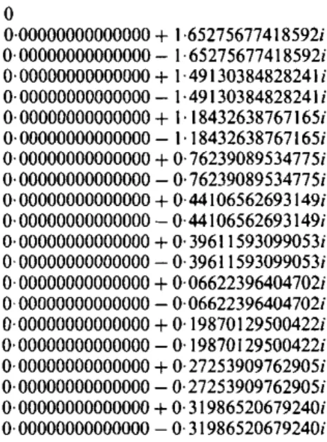
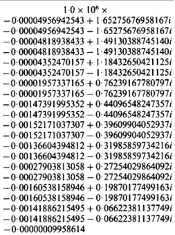
50.

The first 21 eivenvalues of the linearized equations are shown in Tables 1-4. Note that in case (i) the control parameters are set to zero, hence the resulting system is expected to be conservative (see (56». This property is reflected in the system eigenvalues as shown in the Table I, since all eigenvalues are on the imaginary axis. The eigenvalue at the origin is the one associated with the rigid body motion. In cases (ii) -(iv), we gradually increase the control parameters; as a result, the eigenvalues are shifted to the left hand side of the complex plane. The results are given in Tables 2-4, in which negative real eigenvalues are associated with rigid body motion.

Tables 2-4 suggest that the eigenvalue associated with rigid motion and the eigenvalues associated with the flexible beam are separated. Hence, a singular perturbation approach may be employed to separate rigid body and flexible beam motion. This point needs further investigation.

1·0X 106X

o

0·00000000000000 + 1·65275677418592; O· 00000000000000 - I· 65275677418592; 0·00000000000000 + 1-49130384828241;

o-

00000000000000 - 1·49130384828241; 0·00000000000000 + 1·18432638767165;

o.

00000000000000 - I· 18432638767165; 0·00000000000000+0·76239089534775; 0·00000000000000-0·76239089534775; 0·00000000000000+0·44106562693149; 0,00000000000000-0,44106562693149;

o·

00000000000000 +

o-

39611593099053; 0·00000000000000 - 0·39611593099053; 0·00000000000000+0·06622396404702; 0·00000000000000-0·06622396404702; 0·00000000000000+0·19870129500422; 0·00000000000000-0'19870129500422; 0·00000000000000+0·27253909762905; 0,00000000000000-0·27253909762905; 0·00000000000000+0·31986520679240; 0·00000000000000-0·31986520679240;

Table I. Eigenvalues for case(i).

1·0

+

106 _x -0·00000991383610 + 1·65275677400184; -0,00000991383610 - 1·65275677400184; - O' 00000963778897 + 1-49130384984936; -0 00000963778897 - 1-49130384984936; - O' 00000870462923 + 1· 18432639233409; - O· 00000870462923 - I· 18432639233409; - O' 00000391098458 + O'76239092666431; - O'00000391098458 - O'76239092666431; -0,00029570966707 + 0·44106161670923; -0·00029570966707 - 0·44106161670923; -0,00030390996040 + O· 39611526013272; - O'00030390996040 - O'396115260J3272; -0,00027299538539 + O· 31986494317930; -0,00027299538539 - O'319864943J7930; -0·00005579537139 + 0·27253914563337; -0,00005579537139 - 0·27253914563337; -0,00032091615697 + 0·19870131432510; -0,00032091615697 - 0·19870131432510; -0'00028366880576 + 0·06622395795656; - O' 00028366880576 - O'06622395795656; - O'00000000995861

1·0X 106X - 0·00004956942543

+

1 65275676958167i -0·00004956942543 - 1·65275676958167i -0·00004818938433+1·4913038874514Oi -0·00004818938433 - 1·4913038874514Oi -0·00004352470157

+

1·18432650421125i -0·00004352470157 - 1·18432650421125i -0·00001957337165

+

o-

76239 I67780797i -0·00001957337165 - 0·76239167780797i -0·00147391995352

+

0·44096548247357i -0·00147391995352 - 0·44096548247357i -0·00152171037307

+

O· 39609904052937i -0·00152171037307 - O· 39609904052937i - O· 00 136604394812

+

O· 31985859734216i -0· 00 136604394812 - O· 31985859734216i - O· 00027903813058

+

O· 27254029864092i - O· 00027903813058 - O· 27254029864092i -0·00160538158946

+

0·19870177499163i -0·00160538158946 - 0·19870177499163i -0·00141886215495

+

0·06622381 I37749i -0·00141886215495 - 0·06622381137749i - O· 00000009958614

Table 3. Eigenvalues for case (iii).

1·0X 106X - 0·00049594449821 +1·65275628883989i -0·00049594449821 - 1·65275628883989i -0· 00048234201332

+

1-49130771845832i -0· 00048234201332 - 1-49130771845832i -0·00043682107630

+

I· 1843378255601 Ii -0·00043682107630 -1·1843378255601Ii - 0·00021367108258

+

O· 76246472925129i -0·00021367108258 - 0·76246472925129i -0·00985797300231

+

0·43278257310699i - O· 00985797300231 - O· 43278257310699i -0·01728173224534

+

O· 392670058 I6040i -0·01728173224534 - O· 392670058 I6040i -0·01490996309780

+

O· 31894247449221i -0·01490996309780 - O· 3189424744922li -0· 00285657549433

+

O· 27266938442801 i - O· 00285657549433 - O· 2726693844280 Ii - O· 0 1696060 112934

+

O· I9870880407025i -0·01696060112934 - 0·19870880407025i -0·01476250668735

+

0·06620370051114i -0·01476250668735 - 0·06620370051114i -0·00000099586137

Table 4. Eigenvalues for the case (iv).

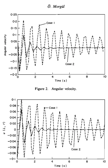
For the purpose of illustration, we simulate the equations of the system% for the following two sets of parameters.

Set I p = I kg rn", GA =693 kg ms", EI =223 kg m"S-2, Ie =0·033 kg m, IR = 100 kg m2, L = 2 m, b = I m: case I:k = 0, ex = 0,

fJ

= 0; case2:k = I, ex = I,

fJ

= I; Set 2 p = I kg m", GA = 1·5 kg mS-2, El = 7·5 kg rrr'S-2,Ie = I kg m, I_R= I kg m2, L

=

O· 1m, b

=

1m: case3: k = 0, ex = 0,

fJ

= 0; case4: k = 1, ex = I,

fJ

= I.

Figures 2- 7 show the simulation results for the rigid body angular velocity00,

the end point deflectionu(L, t)and the end point deflection velocityu,(L, t) in cases 1-4 indicated above. These results show that, in the absence of controls (i.e. cases

(I)and (3)), the beam oscillations do not decay, thus making the flexible spacecraft considered here unsuitable for most applications. However, with the application of appropriate control laws (i.e. cases (2) and (4», these oscillations decay exponen-tially to zero.

788

O.

Morgid 0·25r - - - , -0,15 0·2 f- I II .-Cose I /I 1 l 0'15f-" I ,I ~ , , I I ,I • I II I I " " " /1 , 0'1 I- '~ " I ' \ I I /I , " • A " " " " II 1\ II '\ I I 1\ A 0'051- I, I , I I I I I 1 " , I , \ ' I ' I I,

'I \

II

I " I , I , 1 ' I ' , I ' , ' I , 1,1). I , I ' I , , ' I , I , I , , I \

~

0

t-I,

I"

'~/;'\.\.1-.of"·:-Tji·1·r:-·t-f-tt·Tf-t

'"

'/~'YI"""

" I'

'I"

! .:i -0'05 I

!v

I " I I I, \ , " " '" .. " " I

I "

I' tl "

~

I -0,1

t :,

\1

V

I I I' , I Cose 2 II

,

-0'2 I , , , 0 2 4 6 8 10 Time (s)

Figure 2. Angular velocity.

10 I 8 I 6 I 4 Time (s) 0'1

~

I 0·08 f- ,

r,

,I

~

' 'I II _Cosel 0'06 ~I ' I I , I I I I " . . ~,' II II

' I , , '

~ 0'04 - 0

I

I I,

I

II I I II II

1\

'I ~ • f , I I I " , . , I' A 0·02 i

I

1.\:

I'

I I

I

I I 1

1\

i, : \

n

t\

a

Vii

AI

I \ , I " ' 1 I I , , , , I \ o

"f

v·,

'~'i.n·+-:·-+-·:-t·TI.T1.-r-r-r--H

"-0'02

'I

V

I

I

I

I , I I \ ' I , , : I : \ : \ '

Ii,

I I :: :: :

I

I: :: \/ I'J

V

~'

-0,04

I"

, I I I I \ I " I ' I I I , I I I , I \' \I 'J -0,06 " I

I

,:

V

,

,

\1

\1 I,' Cose 2 -0'08

1

'

I 2 ....

Figure 3. End point displacement.

7. Conclusion

In this paper, we have considered the motion of a flexible beam clamped to a rigid body at one end and free at the other. We have assumed that the centre of mass of the rigid body is fixed in an inertial frame and that the mass of the beam is much smaller than the mass of the rigid body, hence the centre of mass of the rigid body is approximately the centre of mass of the whole configuration. For this configuration, we have first used the so-called geometrically exact beam model for the flexible beam to obtain the equations of motion. We then proposed a feedback control law and showed that, together with this control law, the solutions of the

2,---...,

-1,5 I 1·5

1-,'

I~ I I: II " ~case I 11-1I, II

/I"

II (\

•

, I

"

~ • t!.1 II'! ' I I I ,1 ' \ " t II ~ 0·5 IT I \ I , I I , I I I I , , \ t , 1\ -, 'I o

~-1

f

'·If\

i.{.~-.l~-l.4-7f'

\

·:....:...4·4·L

to '\~.

''1

I ' I I , V " v ! \ ' " \'/ ' '1 1 ' 1 ' 1 , \ / 1 / \ I 1/

v

> " -0'5 f- II~ " I ' \ I

I' , \/ ...

v 1"/ " , ,I ,I L; V _I _ IV, I' / " ~ 1I II I I' II Case 2 I' U ~ I -2 - I

.

...,

-2·5 I I I I 0 2 4 6 8 10 Time (s )

Figure 4. End point velocity.

,.,

~ u .Q

"

> A ~ II Case 3 I' I ,I II ,~ I ~, ,I 'I ' II ! 0'5 f- II I \

,I

~

(\

I ~ 1\ ,

,I',

/I , ,

q " "

I, " "I ,1

1\ h

,'II:

I , \ '\ " I I ,I

I'

'I "" A,I

I':

I I ' I rI rI , \ " : I I , I I I I I II ',I'll""

,u,

I I I, I I , I I ' " , o 1\, I , , , I , ,

""'1/11'"

I ' " I '~, I ,

!

r.L.J....l I I I I ' I I I , I I II " II

!i.iL

+1-1J.-4- •t-""'"J1j"""'""1" •..,--: , I, \I I I

u-t~H-vT"

': ::

\,'1' :' \

I \: : I : .2 I I,

!

L "

I

1/'"

" I , \' ' : I I I' II II ,

s

-0,5

I

~'IiI \, ~ ' \, V I Ir Ir

II

~I ,I

.:i

1"

I' I' I I II II ~ I ~

,

t 1/ II ~ - I Case 4 I 2 I 4 6 Time (s) I 8

Figure 5. Angular velocity.

equations of motion are stabilized in the sense that the 'energy' of the configuration becomes a non-increasing function of time.

Under the assumption of planar motion linearization of the geometrically exact beam model yields the well-known Timoshenko beam model. By using this lin-earized model for the beam, we then showed that with the proposed control law, the 'energy' of the configuration, decays exponentially to zero.

Whether we can obtain exponential stabilization by using the geometrically exact beam model without any linearization needs further investigation. Also, application of the boundary control techniques presented in this paper to various problems arising in the control of flexible structures, such as tracking, orientation. etc., could prove useful.

790

O.

Morgiil 1·2 0·8 0·4 0·6 Time (s) 0·2 ,.~ I I I \ ;'-_ ... I I--Case 3 I \ I \ " I \ " I \ I ' I \ f I I \ 1 ' f /".~ \ I , ~ -' --l._ f / \ f \ I , \ I \ I rcose4 ', f \

//'

, , /

'

I ~ I

'I

I ' ~ I

1/

" /

',

I' -0-5 004 0-3 0'2

-

-

0·1

-... 0 ~ _-0'1 -0'2 -0,3 -0-4 -0-5 0

Figure 6. End point displacement.

15r - - - , I I I 0·8 I 0·6 Time (s) I 0·2 I~I 10 " I , 1I I , f I r ,

_{\ ' / v ,}

r....-Cose 3

f ,

f ,

5

ft...."

f I

f ,...-.'\.

CLose

4,'

\

Of- ' \ »: -+----~._---, , • ../ I , I \ I , \ / ..."-" \ I I f ' I I I \ I \ I \ I ... -\ I

\../

I 0'4 -5 f--10

f-Figure 7. End point velocity. ACKNOWLEDGMENTS

The author would like to thank Professor Charles A. Desoer for his guidance, encouragement and careful review of this manuscript, and John Anagnost for many helpful discussions and numerous helpful comments. The author also gratefully acknowledges the help of Ogan Ocah for the simulation results presented in the manuscript.

This research has been partially supported by National Science Foundation Grant ECS 8500993 and by the Scientific and Technical Research Council of Turkey.