A DISSERTATION SUBMITTED TO
THE GRADUATE SCHOOL OF ENGINEERING AND SCIENCE OF BILKENT UNIVERSITY
IN PARTIAL FULFILLMENT OF THE REQUIREMENTS FOR THE DEGREE OF
DOCTOR OF PHILOSOPHY IN
ELECTRICAL AND ELECTRONICS ENGINEERING
By Berk Osunluk February 2021
February 2021
We certify that we have read this dissertation and that in our opinion it is fully adequate, in scope and in quality, as a dissertation for the degree of Doctor of
Philosophy.
Elane}
{)2{,ay
KAdvisor)B. Orhan Aytilr
Co~kun Kocab~
Approved for the Graduate School of Engineering and Science:
Ezhan Kara~an
Director of the Graduate School
iii
ENVIRONMENTAL EFFECTS ON INTERFEROMETRIC FIBER OPTIC GYROSCOPE PERFORMANCE
Berk Osunluk
Ph.D. in Electrical and Electronics Engineering Advisor: Ekmel Özbay
February 2021
Today main performance limitations for fiber optic gyroscope technology are its sensitivity to temperature fluctuations and vibration. Shupe error is the main error source for both disturbances. We propose an approach to reduce the thermal sensitivity by controlling the strain inhomogeneity through the fiber coil. The approach is based on advanced fiber coil modeling, which is verified by a series of experiments.
Vibration is often a neglected disturbance by the researchers as it highly depends on the integrated platform. We propose a model for bias error formation due to optical power fluctuations under vibration. Model is composed of power fluctuation characteristics, spurious rotation rate formation due to mechanical Shupe error, and the suppression of the rotation rate by the closed-loop operation. Lastly, we introduce the concept of angle random walk performance degradation under vibration due to interferogram nonlinearity.
Keywords: Fiber optic gyroscope, Shupe error, Thermal sensitivity, Vibration, Bias, Angle random walk (ARW), Interference nonlinearity.
iv
ÖZ
GİRİŞİMÖLÇÜCÜ FİBER OPTİK DÖNÜÖLÇER PERFORMANSI ÜZERİNE ÇEVRESEL ETKİLER
Berk Osunluk
Elektrik-Elektronik Mühendisliği, Doktora Tez Danışmanı: Ekmel Özbay
Şubat 2021
Günümüzde fiber optik dönüölçer teknolojisi için temel performans limiti sıcaklık hassasiyeti ve titreşimdir. Shupe hatası her iki bozanetken için de temel hata kaynağıdır. Fiber sarımdaki gerinim tektürelsizliğini kontrol ederek sıcaklık hassasiyetini düşüren bir yaklaşım öneriyoruz. Yaklaşım, bir dizi deney ile doğrulanmış ileri seviye bir modellemeye dayanmaktadır.
Titreşim entegre edilen platforma bağlı olduğu için çoğunlukla araştırmacılar tarafından göz ardı dilen bir bozanetkendir. Titreşim altında optik güç salınımları nedeniyle oluşan sabit hata için bir model öneriyoruz. Model optik güç salınım karakteristikleri, mekanik Shupe hatası nedeniyle sahte dönü hızı oluşumu, ve kapalı döngü opearsyon ile dönü hızı baskılanmasını içermektedir. Son olarak girişimölçer doğrusalsızlığı nedeniyle titreşim altında açısal rastgele yürüme performans düşüşünü tanıtıyoruz.
Anahtar sözcükler: Fiber optik dönüölçer, Shupe hatası, Sıcaklık hassasiyeti, Titreşim, Sabit hata, Açısal rastgele yürüme (ARW), Girişim doğrusalsızlığı.
v Annem’e
vi
ACKNOWLEDGEMENT
A decade ago, the fiber optic gyroscope jumped into the middle of my professional life and meanwhile, it feels like a child. This thesis is a rite of passage. From now on, our relation will be much more stable, and I may save more time for my beloved toddler, Uygar.
Creating this dissertation was not a personal experience, definitely a collective one, and I owe gratitude to a lot of people. First and foremost, I would like to express my sincerest gratitude to my advisor Prof. Ekmel Özbay for his invaluable guidance. I would also like to extend my gratitude to Dr. Burak Seymen for his highly innovative contributions, especially for Chapter 4. My special thanks go to my academic buddy Serdar Öğüt, without whom the thesis may not come true.
This thesis is funded by SSB (Savunma Sanayii Başkanlığı) and Aselsan Inc. with a SAYP (Savunma Sanayii için Araştırmacı Yetiştirme Programı) project. I am very grateful for the resources and facilities that were made available to me during my studies. I would like to send my warm thanks to each of my family members, but especially to my father, for their continuous support, not only for this thesis but also for my life. Last, but certainly not least, I would like to thank my wife Gülçin for her non-stop support, patience, and help. Her existence makes everything much more meaningful, without which not only this thesis but also anything will be harder.
“. . . Our sons ought to study mathematics and philosophy, . . . navigation, . . . in order to give their children a right to study painting, poetry, music . . .” J. Adams
vii
CHAPTER 1: INTRODUCTION ... 1
CHAPTER 2: BASICS OF FOG ... 4
2.1 Sagnac Scale Factor ...4
2.2 Interference of Waves ...6
2.3 Minimum FOG configuration ...8
2.4 Phase modulation/demodulation ...9
2.5 Closed-Loop Configuration ... 11
2.6 Performance Parameters ... 13
2.6.1 Bias Error ... 13
2.6.2 Scale Factor Stability ... 14
2.6.3 Angle Random Walk (ARW) ... 14
CHAPTER 3: THERMAL SENSITIVITY ... 15
3.1 Review of Theory ... 16
3.1.1 Shupe Bias Drift ... 16
3.1.2 Elastooptic Bias Drift ... 19
3.2 Modeling Approaches in the Literature ... 22
3.2.1 Obtaining the Temperature and Strain Fields ... 22
3.2.2 Winding Method ... 24
3.2.3 Repetition of a Literature Model... 27
3.3 Advanced Modeling of the Fiber Coil ... 39
3.3.1 Homogenization / Dehomogenization Procedure ... 40
3.3.2 Coil Winding Pattern ... 42
3.3.3 Bias Error Calculation Approach ... 44
3.3.4 Simulations and Results of the Advanced Model ... 45
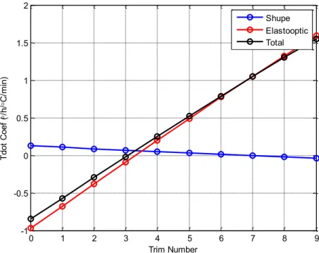
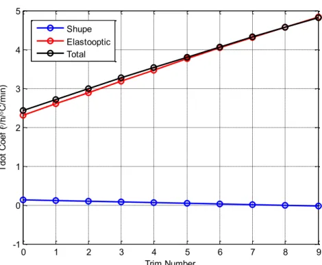
3.3.5 Trimming ... 54
3.4 Strain Distribution through the Coil ... 59
3.4.1 Strain Analysis Approach ... 59
viii
3.4.3 Elongation vs. refractive index change ... 63
CHAPTER 4: VIBRATION ERROR ... 70
4.1 Optical Power Fluctuation ... 70
4.1.1 Optical Power Fluctuation and Rate Error are in Phase ... 71
4.1.2 Optical Power Fluctuation and Rate Error are out of Phase ... 76
4.1.3 Rate Error for a Closed-Loop FOG ... 78
4.1.4 Optical Power Fluctuation Estimation with Simulation and Test ... 81
4.2 Mechanical Shupe Error ... 85
4.2.1 Tests for Mechanical Shupe Error ... 88
4.3 Interferogram Nonlinearity ... 89
4.3.1 FOD Discrete Model ... 92
4.3.2 Simulations for ARW Performance ... 94
4.4 Vibration Tests at High Sampling Rate ... 99
CHAPTER 5: CONCLUSION ... 103
ix
Figure 2.1: Sagnac effect. ... 5
Figure 2.2: Rotation rate sensing device. ... 8
Figure 2.3: Open-loop FOG configuration. ... 9
Figure 2.4: Digital ramp for loop closure. ... 12
Figure 2.5: Closed-loop FOG configuration. ... 13
Figure 3.1: Shupe effect. ... 17
Figure 3.2: Axis definition through the fiber ... 20
Figure 3.3: Thermal stress on the fiber core due to coating expansion [36]. ... 23
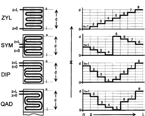
Figure 3.4: Four different fiber coil winding methods, ZYL: Cylinder, SYM: symmetric, DIP: dipole, QAD: Quadrupole [32]. ... 25
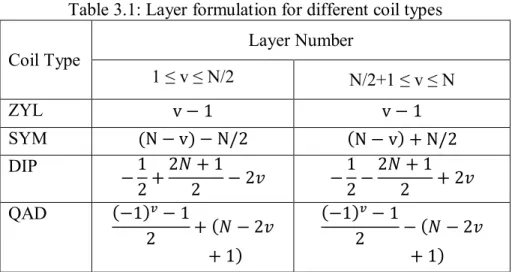
Figure 3.5: Steps in the winding of a quadrupole coil [44]. ... 27
Figure 3.6: Coil model. ... 28
Figure 3.7: Quadrupole winding pattern. ... 29
Figure 3.8: Temperature profiles. Reference [38] (left) and the simulation (right). .... 34
Figure 3.9: Temperature distribution through the fiber coil. ... 35
Figure 3.10: Temperature derivative distribution through the fiber coil. ... 35
Figure 3.11: Stress distribution through the coil radial axis. ... 36
x
Figure 3.13: Stress distribution through the coil axial axis... 37
Figure 3.14: Bias error estimations vs the coil temperature... 38
Figure 3.15: Bias error estimations. Reference [38] (left) and the simulation (right). . 38
Figure 3.16: Fiber coil is an orthotropic composite material [39]. ... 40
Figure 3.17: Fiber coil RVE. Fibers are located in an orthocyclic manner with adhesive in between. All dimensions are in µm. ... 40
Figure 3.18: Simulation of RVE with high resolution meshed. ... 41
Figure 3.19: Practical Quadrupole Pattern. ... 44
Figure 3.20: FEM model of the fiber coil. ... 46
Figure 3.21: Input temperature profile is obtained from the laboratory experiments. . 48
Figure 3.22: Temperature distribution through the fiber coil... 49
Figure 3.23: Temperature derivative distribution through the fiber coil. ... 49
Figure 3.24: Strain (radial) distribution through the fiber coil. ... 50
Figure 3.25: Strain (axial) distribution through the fiber coil. ... 51
Figure 3.26: Bias error estimations. ... 51
Figure 3.27: Setup for FOG thermal sensitivity experiments. ... 52
Figure 3.28: Bias error measurements and simulation estimation vs fiber coil temperature. ... 53
Figure 3.29: (a) Perfect trimming case for quadrupole winding (b) imperfect case, the position of the midpoint is changed [42]. ... 54
xi
Figure 3.31: Trimming results for Coil Design #1, with practical quadrupole pattern. 57
Figure 3.32: Trimming results for Coil Design #2, with practical ideal pattern. ... 58
Figure 3.33: Trimming results for Coil Design #2, with practical quadrupole pattern. 59 Figure 3.34: FEM simulation of the fiber coil model. Fiber coil dimensions are in mm. High stress region is in the coil spool intersection. ... 60
Figure 3.35: Stress distribution through the fiber coil. Temperature changes as time progresses. ... 61
Figure 3.36: Strain (through the fiber propagation axis) distribution with respect to time and the turn number. ... 65
Figure 3.37: (a) Total strain change of the fiber coil. Simulation output for each temperature point is compared with the OTDR measurement of a fiber coil. (b) Calculated strain temperature coefficient for each turn number. ... 65
Figure 3.38: Radial and axial mean strain temperature coefficients for different spool configurations. ... 67
Figure 3.39: Radial and axial mean strain temperature coefficients for Coil Design #1, 2, and 3. ... 68
Figure 3.40: Simulated and experimental bias error curves. ... 69
Figure 4.1: FOG discrete time model and controller diagram. ... 78
Figure 4.2: Stability of the system for different controller gains. ... 79
xii
Figure 4.4: Error response. ... 81
Figure 4.5: FOG data under vibration test. ... 82
Figure 4.6: Phase and bias errors vs vibration input level. ... 84
Figure 4.7: Mechanical Shupe error simulation. Linear vibration is transformed into spurious rotation rate due to mechanical Shupe error... 88
Figure 4.8: PSD of FOG output under different vibration energy levels. ... 89
Figure 4.9: Input vs FOG model output. Here asin is modeled as asin(x) = x, i.e. with error. ... 95
Figure 4.10: Power spectral density of MIL-STD-810G Figure 514.6D-1 Category12 [47]. ... 96
Figure 4.11: Power spectral density of the induced rotation ... 97
Figure 4.12: Gyroscope output power spectral density. ... 99
Figure 4.13: PSD for different rate estimations. ... 101
xiii
Table 3.1: Layer formulation for different coil types ... 26
Table 3.2: Coil Parameters [38] ... 33
Table 3.3: Modeling Parameters (Adapted from [38]) ... 33
Table 3.4: Coil parameters ... 46
Table 3.5: Coil parameters obtained by homogenization ... 47
Table 3.6: Dehomogenization parameters ... 47
Table 3.7: Temperature derivative sensitivity coefficients ... 53
Table 3.8: Coil parameters for trimming simulations ... 56
Table 3.9: Von Mises stress values for different spool materials ... 61
Table 3.10: Coil design parameters for strain analyses ... 62
Table 3.11: Error contributions ... 63
Table 4.1: Bias error and rotation rate measurements, and uncompensated phase error estimation ... 83
Table 4.2: Controller error response vs controller gain ... 85
Table 4.3: Amplitudes of frequency components... 91
Table 4.4: ARW of open-loop FOG configuration for different input amplitudes ... 95
Table 4.5: ARW for different asin approximations ... 97
xiv
LIST OF ALGORITHMS
Algorithm 3.1: Matlab code for bias error calculations ... 29
Algorithm 4.1: Controller response ... 81
1
CHAPTER 1
INTRODUCTION
Today, interferometric fiber optic gyroscope (IFOG, or FOG as commonly used) technology is 45 years old [1]. It has been integrated into many different platforms operating in various environments, including air, naval, and land vehicles, deep drilling platforms, and even space [2], [3], [4]. Today, the trend is towards seeking excellence under different environmental effects. Environmental effects include moisture [5], radiation [6], [7], magnetic field [8], [9], vibration, and temperature fluctuation. The first three disturbances may be suppressed by simple mechanical solutions. Moisture level can be controlled by a hermetically sealed case. Radiation hardened fibers and electro-optic parts are proposed for robust FOG configurations for space applications. The magnetic field effect can be suppressed by a shield having high permeability and covering the Sagnac loop. However, the temperature fluctuations and vibration may limit the performance of FOG; even thermal or mechanical isolators are used.
This dissertation is devoted to defining the performance limitations of FOG due to temperature and vibration effects. Chapter 2 covers the basic principles and structure
2
of commonly used FOG configuration. Shupe equations are direct results of the Sagnac relation. The modulation/demodulation scheme and closed-loop configuration of FOG should be reviewed for a better understanding of the vibration error due to optical fluctuations. Lastly, the interference of the waves forms the basis of the interferogram nonlinearity analyses.
Chapter 3 starts by sketching the panorama of the thermal sensitivity of the FOG coil. Literature work is handled by both referring and repeating it with similar models and simulation scenarios to underline the need for an advanced model. The advanced modeling approach is presented in detail and verified by laboratory experiments. The trimming phenomenon is revisited with simulations. Lastly, different thermal bias error contributions are analyzed and strain inhomogeneity analysis is presented for further improvement of fiber coil. A fiber coil design is reached, showing that the approach proposes simple design changes to increase the performance to the same order of magnitude as the latest developments in the literature. Performance is better than various quadrupole designs [10], [11], [12] and close to octupolar winding performance [11], [12].
Chapter 4 is dedicated to FOG performance under vibration. Vibration, as a disturbance, is highly dependent on the platform on which the sensor is integrated into. Characteristics of the vibration like the frequency range, magnitude, and occurrence rate change dramatically for different vehicles, terrains, and operation concepts. Furthermore, mechanical isolators for the suppression of the vibration may be designed according to the platforms during the integration phase. So, the inertial sensor performance under the vibration is often a neglected issue in the academic literature, sensor tests under vibration are deferred until the integration phase of the project, and engineers/researchers are sleeping on the issue during the design phase. However, the vibration can be the limiting factor of the inertial sensor performance. Today, one of the main limitations of FOG performance is its sensitivity to vibration. Vibration is a time-dependent disturbance on the fiber sensing coil, similar to the
3
temperature, which results in performance degradation. Several literature works focus on the mechanical Shupe error [13], [14], [15], [16], [17] and some the effect of the optical power fluctuation [18], [19]. The mechanical Shupe error is much more investigated and modeled than the latter one.
Detailed analyses of error formation due to optical power fluctuation for different cases are presented in Chapter 4. Error occurs in two different forms: Bias error and Shupe like error. Both errors depend on the multiplication of the Sagnac phase shift with power fluctuation. Bias error exists if only the two signals are in phase. Chapter 4 proceeds to closed-loop configuration and mechanical Shupe error. Sagnac phase shift is a multiplicative term in error equations and closed-loop suppresses the phase shift. The effectiveness of the loop closure, which can often be neglected in the literature, is modeled and part of the optical power estimations in experiments part.
One of the important parts of Chapter 4 is about the non-linear fashion of the interferogram. Nonlinearity creates low frequency error in the FOG output, although no input energy exists at those frequencies. The noise floor of the gyroscope increases under vibration which results in the angle random walk (ARW) performance degradation. The theoretical proposal is supported by the simulations and laboratory experiments of a FOG. To the best of our knowledge, this dissertation is the first literature work about this phenomenon.
4
CHAPTER 2
BASICS OF FOG
FOG measures the phase shift between two light waves counter-propagating through a rotating loop of fiber. Rotation induces a phase shift between the waves, called the Sagnac effect [20], [21]. This effect depends on the Einstein’s special theory of Relativity, although Sagnac explains his experiment as a demonstration of the Aether theory, which bases on the Fresnel-Fizeau drag effect. Von Laue explained the Fresnel-Fizeau drag effect as a relativistic effect by considering the first-order solution of the law of addition of speeds of special Relativity for a medium [2].
The Sagnac phase shift between the counter-propagating waves can be measured with an interferogram. The rotation rate is obtained by measuring the power level of the interfering waves.
2.1 Sagnac Scale Factor
Two counter-propagating waves in a fiber loop experience a relative phase shift while the loop rotates about its symmetry axis (Figure 2.1). Counter-propagating
5
waves enter the loop at the same time with identical phases. The shift of the exit point due to rotation causes one of the waves to exit the loop earlier and the other one later.
Figure 2.1: Sagnac effect.
Time difference between the waves due to rotation,
𝑡𝑐𝑤 = 𝑅(2𝜋 + Ω𝑡𝑐𝑤) 𝑐 (2.1) 𝑡𝑐𝑐𝑤 = 𝑅(2𝜋 − Ω𝑡𝑐𝑐𝑤) 𝑐 (2.2)
where 𝑡𝑐𝑤 and 𝑡𝑐𝑐𝑤 are propagation times of clockwise (CW) and counter- clockwise (CCW) waves respectively. 𝑅 is the radius of the fiber coil loop, Ω is the rate of rotation, and 𝑐 is the velocity of light in vacuum. The time difference is,
6
Δ𝑡 = 4𝜋Ω𝑅
2 𝑐2− Ω2𝑅2
(2.4)
A number of loops of fiber can be wound on a fiber coil to enhance the effect. Multiplying the equation with number of loops 𝑁 and by using the approximation 𝑐2 ≫ Ω2𝑅2, Δ𝑡 =4𝜋Ω𝑅 2𝑁 𝑐2 (2.5) Δ𝑡 =𝐿𝐷Ω 𝑐2 (2.6)
where, 𝐿 is the length and 𝐷 is the diameter of the fiber coil. Waves travel the loop with the angular velocity 𝜔 =2𝜋𝑐
𝜆 , where 𝜆 is the wavelength in vacuum. Phase difference between the waves due to the Sagnac effect becomes,
Δ𝜙 =2𝜋𝐿𝐷
𝜆𝑐 Ω (2.7)
This linear coefficient between the rotation rate and the phase shift is named Sagnac Scale Factor. Equation (2.7) also applies to the fiber medium where c and 𝜆 values are still for the vacuum.
2.2 Interference of Waves
Two coherent counter-propagating waves interfere and create an optical power shift due to the phase difference between the waves. The Sagnac effect can be measured by using an interferometer. Two monochromatic waves with a phase difference can be defined as,
7
𝐸1(x, t) = 𝐸10𝑦̂𝑠𝑖𝑛(𝑘𝑥 − 𝜔𝑡) (2.8)
𝐸2(x, t) = 𝐸20𝑦̂𝑠𝑖𝑛(𝑘𝑥 − 𝜔𝑡 + Δ𝜙) (2.9)
where 𝑘 is the wave vector,
𝐸10 and 𝐸20 are electric field intensities,
and 𝑦̂ is the unit vector.
Time averaged optical power output of the interference of the waves can be computed as, 𝑃(𝑥, 𝑡) = 𝑐𝜀0|𝐸1(x, t) + 𝐸2(x, t)|2 (2.10) 𝑃(𝑥, 𝑡) = 𝑐𝜀0[𝐸10 2 2 + 𝐸202 2 + 〈2𝐸10𝐸20𝑠𝑖𝑛(𝑘𝑥 − 𝜔𝑡)𝑠𝑖𝑛(𝑘𝑥 − 𝜔𝑡 + Δ𝜙)〉] (2.11) 𝑃(𝑥, 𝑡) = 𝑐𝜀0[ 𝐸102 2 + 𝐸202 2 + 𝐸10𝐸20〈𝑐𝑜𝑠(Δ𝜙) − 𝑐𝑜𝑠(2𝑘𝑥 − 2𝜔𝑡 + Δ𝜙)〉] (2.12) 𝑃(𝑥, 𝑡) = 𝑃1+ 𝑃2+ 2√𝑃1𝑃1𝑐𝑜𝑠(Δ𝜙) (2.13)
where 𝑃1 and 𝑃2 are the average optical power of the two interfering waves. Under the assumption of 𝑃1 = 𝑃2,
8 𝑃(𝑥, 𝑡) = 𝐼0
2 [1 + 𝑐𝑜𝑠(Δ𝜙)]
(2.14)
where 𝐼0 is the maximum optical power, i.e. when Δ𝜙=0.
2.3 Minimum FOG configuration
A rotation rate measurement setup can be formed by using a light source for the light wave creation, a coupler to divide the light wave into counter-propagating waves, a fiber coil to obtain the Sagnac effect, and a detector to convert the optical power due to interference into current (Figure 2.2). Rate measurement can be obtained with this simple configuration. Optical power remains at maximum in the no-rotation case and it decreases under any rotation, CW or CCW, which states the lack of the direction information of the rotation rate input.
Figure 2.2: Rotation rate sensing device.
Phase modulation is the common way to overcome this problem. Phase bias is injected between the waves using a phase modulator. Multifunctional integrated optical chip (MIOC) and piezoelectric transducer (PZT) are two widely used phase modulators for injecting a phase shift. Although there are several FOGs making use of PZT in the market, MIOC is much more preferred due to its much higher bandwidth and phase stability.
9
Besides the phase bias injection, the configuration of a FOG should be reciprocal [22]. The reciprocal configuration ensures the waves travel the same optical path so that only the Sagnac effect results in a phase delay. Reciprocal configuration brings the need for using a second coupler.
Lastly, the fiber has a slightly anisotropic structure: Optical path length and the refractive index is different for the waves with orthogonal polarization states. If both of the polarization states are let to propagate through the loop, then spurious waves interfere at the detector with a birefringence phase shift rather than the Sagnac phase shift. Using a polarizer in the optical path is a solution for this problem [22]. Figure 2.3 shows the minimum FOG configuration including a polarizer, second coupler, phase modulator, and bias modulation/demodulation electronics.
Figure 2.3: Open-loop FOG configuration.
2.4 Phase modulation/demodulation
Square wave modulation is a commonly used modulation technique for high performance FOGs. The objective of injecting phase bias is achieved by the use of a reciprocal phase modulator placed at one end of the coil that acts as a delay line (Figure 2.3). Both interfering waves carry exactly the same phase modulation due to
10
the reciprocity, except for a shift in time. The time shift between the waves exactly equals the coil-loop transit time of the waves if the phase modulator is placed at one of the ends of the fiber loop. Two waves enter the coil in counter directions after their split at the coupler. One of the waves experiences the phase shift injected at the phase modulator while the second one experiences after traveling the fiber coil. Coil transit time is calculated as
𝜏 =𝑛𝐿 𝑐
(2.15)
where L is the fiber coil length, c is the light velocity and n is the refractive index of the medium. Induced phase shift is
Δ𝜙𝑚(𝑡) = 𝜙𝑚(𝑡) − 𝜙𝑚(𝑡 − 𝜏) (2.16)
A square wave with coil transit time half period and Δ𝜙𝑚/2 amplitude can be used.
𝜙𝑚(𝑡) = { Δ𝜙𝑚 2 , 0 ≤ 𝑡 < 𝜏 −Δ𝜙𝑚 2 , 𝜏 ≤ 𝑡 < 2𝜏 (2.17) Δ𝜙𝑚(𝑡) = { Δ𝜙𝑚, 0 ≤ 𝑡 < 𝜏 −Δ𝜙𝑚, 𝜏 ≤ 𝑡 < 2𝜏 (2.18)
Equation (2.6) can be rewritten for the two cases,
𝑃0 =𝐼0
2[1 + cos(Δ𝜙𝑠(𝑡) + Δ𝜙𝑚)]
11 𝑃1 =𝐼0
2[1 + cos(Δ𝜙𝑠(𝑡 + 𝜏) − Δ𝜙𝑚)]
(2.20)
The Sagnac phase shift can be reconstructed by square wave demodulation.
Δ𝑃 = 𝑃1− 𝑃0 (2.21)
The Sagnac phase shift change can be assumed to be much slower than the transit time so Δ𝜙𝑠(𝑡 + 𝜏) ≅ Δ𝜙𝑠(𝑡) can be assumed.
Δ𝑃 =𝐼0 2[2𝑠𝑖𝑛(Δ𝜙𝑠)𝑠𝑖𝑛(Δ𝜙𝑚)] (2.22) Δ𝜙𝑠 = 𝑎𝑟𝑐𝑠𝑖𝑛 ( Δ𝑃 𝐼0𝑠𝑖𝑛(Δ𝜙𝑚)) (2.23)
2.5 Closed-Loop Configuration
Scale factor of FOG should be linear (i.e. independent of the input) and stable under environmental effects. Equation (2.23) is a nonlinear function due to arcsin. Furthermore, optical power could fluctuate easily with temperature. Closed-loop operation is introduced to overcome these effects. Phase modulator can also be used as a feedback device to cancel out the measured Sagnac phase shift between the counter-propagating waves.
𝑃(𝑡) =𝐼0
2[1 + 𝑐𝑜𝑠(Δ𝜙𝑠(𝑡) + Δ𝜙𝑚(𝑡) − Δ𝜙𝑓(𝑡))]
(2.24)
12
Δ𝜙𝑓(𝑡) = 𝜙𝑓(𝑡) − Δ𝜙𝑓(𝑡 − 𝜏) = −Δ𝜙𝑠(𝑡) (2.25)
This equation can be implemented with a digital ramp signal. Ramp dwells at each feedback level for coil transit time duration.
𝜙𝑓(𝑡) = 𝜙𝑓(𝑡 − 𝜏) − Δ𝜙𝑠(𝑡) (2.26)
Figure 2.4: Digital ramp for loop closure.
Figure 2.4 shows the digital ramp which must be reset as the voltage level cannot increase indefinitely. These resets may create an error unless the reset amplitude equals to an integer multiple of 2π. If Δ𝜙𝑓(𝑡) = −(Δ𝜙𝑠± 2𝜋), then the cosine term in Equation (2.24) nulls the reset term. Reset amplitude can be set to any multiplicand of 2𝜋 up to the maximum applicable voltage to the phase modulator. Any gain error in the feedback path results in an error on the reset amplitude [23]. This can be solved with double closed-loop algorithms [24], [25] and four state bias modulation techniques [26].
13
Figure 2.5: Closed-loop FOG configuration.
The closed-loop FOG scheme is given in Figure 2.5. Optical power measured from the photodiode is amplified and converted into voltage by a pre-amplifier. Then an analog to digital converter (ADC) is used to demodulate the signal. The demodulated Sagnac phase is integrated and fed back to the phase modulator. The rotation rate output is the feedback signal. Different controller designs can be used for the loop closure.
2.6 Performance Parameters
Many performance parameters can be defined for FOG as an inertial sensor [27], [28]. Three of the parameters are the most widely referred and directly related to the environmental effects: Bias Error, Scale Factor Stability, and ARW.
2.6.1 Bias Error
Bias error is simply the measurement offset of the sensor. The offset is independent of the rotation rate input as a part of the definition. Gyroscope overall performance is usually defined by the bias error performance. Tactical grade gyroscopes have around 1 °/h bias stability and navigation grades are less than 0.01 °/h. Bias error of
14
FOG is highly sensitive to the environmental effects. Main bias error mechanisms are phase modulator nonlinearity, intensity modulation, Kerr Effect, Faraday Effect, secondary waves due to backscattering and polarization cross coupling, and Shupe Effect [29]. The last one is one of the main concerns in this dissertation.
2.6.2 Scale Factor Stability
Scale factor of a FOG is the ratio of the output per input rotation rate. The scale factor is desired to be perfectly constant, i.e. gyro signal changes linearly with rotation rate and independent of the environmental effects. Any mechanism that results in an error relative to the input could be classified as the scale factor error. Closed-loop configuration increases the scale factor linearity and stability as mentioned in Chapter 2.5. Mean wavelength is a multiplicative term in Equation (2.7), the Sagnac scale factor. The wavelength stability of the light source is one of the main scale factor instability mechanisms for FOG.
2.6.3 Angle Random Walk (ARW)
Noise consists of statistical, non-deterministic, high frequency fluctuations on FOG rotation rate measurement output. Noise is named as ARW as it results in a random walk in the angle estimation. In early fiber gyros major source of noise was due to Rayleigh backscattering. A portion of the light is scattered backward and is captured by the fiber and propagated back to the detector. The advent of broadband (low coherence) light sources permitted the elimination of this type of noise source [30]. Relative intensity (RIN), TIA, shot, thermal, and driver electronics can be named as the main noise sources.
15
CHAPTER 3
THERMAL SENSITIVITY
Performance of FOG has been shown to be sensitive to the thermal gradients across the fiber sensing coil by Shupe [31] in 1980 and this phenomenon is called the Shupe effect since then. The second major step was the introduction of the bias error due to the elastooptical interactions [13]. Thermal sensitivity is suppressed to a degree by various winding methods [32], [33]. Novel fiber technologies are introduced to FOG for lower thermal sensitivity [34], [35]. Despite all these attempts, today, the thermal sensitivity of FOG is still a concern. There are plenty of works in the literature about modeling the error [36], [37], [38], [39], [40], [41], [42]. Obtaining a verified simulation environment opens the road for easier analysis of different types of fiber sensing coil schemes, improvement methods or optimum adhesive selection. We present an advanced modeling approach after revisiting a method in the literature by simulations. We give numerical results of various bias error contributions inside the fiber coil. We propose an approach for reducing the strain inhomogeneity inside the fiber coil to reduce the bias error. A coil design performance, which is comparable to the latest developments, is reached and demonstrated by laboratory experiments.
16
3.1 Review of Theory
3.1.1 Shupe Bias Drift
Light wave experiences a phase shift, Δφ, inside a fiber optic cable with length 𝐿 and refractive index 𝑛, due to a change in the corresponding parameter, Δ𝐿 or Δ𝑛.
Δ𝜑 = 𝛽0𝑛Δ𝐿 + 𝛽0Δ𝑛𝐿 (3.1)
where 𝛽0= 2𝜋
𝜆0, free space propagation constant, 𝜆0 is the wavelength of the light
wave at vacuum.
The change can be induced by environmental effects like temperature [31], vibration [15], or moisture [5]. The total phase shift due to the temperature change is the integral of all infinitesimal fiber portions under the varying temperature field.
Δ𝜙 = 𝛽0𝜕𝑛 𝜕𝑇∫ Δ𝑇(𝑧)𝑑𝑧 𝐿 0 + 𝛽0𝑛𝛼 ∫ Δ𝑇(𝑧)𝑑𝑧 𝐿 0 (3.2) Δ𝜙 = 𝛽0( 𝜕𝑛 𝜕𝑇+ 𝑛𝛼) ∫ Δ𝑇(𝑧)𝑑𝑧 𝐿 0 (3.3) 𝜕𝑛
𝜕𝑇, refractive index thermal coefficient 𝛼, thermal expansion coefficient
Δ𝑇(𝑧), Temperature change along the fiber portion 𝑧
and 𝑛𝛼 is negligible with respect to 𝜕𝑛 𝜕𝑇. [32]
17
A fiber loop geometry is given in Figure 3.1, where the CW and CCW light waves travel the loop. CW wave passes a fiber section 𝑑𝑧 at time 𝑡′ = 𝑡 −(𝐿−𝑧)
𝑐 , with 𝑐 = 𝑐0
𝑛.
Figure 3.1: Shupe effect.
Integrating over all fiber loop results in extra phase shift due to temperature change for the CW wave, and the CCW,
Δ𝜙𝐶𝑊(𝑡) = 𝛽0(𝜕𝑛 𝜕𝑇+ 𝑛𝛼) ∫ Δ𝑇(𝑧, 𝑡 − (𝐿 − 𝑧) 𝑐 )𝑑𝑧 𝐿 0 (3.4) Δ𝜙𝐶𝐶𝑊(𝑡) = 𝛽0(𝜕𝑛 𝜕𝑇+ 𝑛𝛼) ∫ Δ𝑇(𝑧, 𝑡 − 𝑧 𝑐)𝑑𝑧 𝐿 0 (3.5)
The phase difference between the counter-propagating waves becomes,
Δ𝜙(𝑡) = 𝜙𝑐𝑤(𝑡) − 𝜙𝑐𝑐𝑤(𝑡) (3.6) Δ𝜙(𝑡) = 𝛽0(𝜕𝑛 𝜕𝑇+ 𝑛𝛼) ∫ [Δ𝑇 (𝑧, 𝑡 − (𝐿 − 𝑧) 𝑐 ) − Δ𝑇 (𝑧, 𝑡 − 𝑧 𝑐)] 𝑑𝑧 𝐿 0 (3.7)
18
Using the definition of the time derivative: ḟ = limΔt→0[𝑓(𝑡+Δ𝑡)−𝑓(𝑡)] Δ𝑡 Δ𝜙(𝑡) =𝛽0 𝑐0( 𝜕𝑛 𝜕𝑇+ 𝑛𝛼) ∫ 𝑇̇(𝑧, 𝑡)(𝐿 − 2𝑧)𝑑𝑧 𝐿 0 (3.8) can be written.
The FOG works on the Sagnac principle, which states that the rotation of the fiber loop creates a phase difference between the waves with the following relation.
Δ𝜙 =2𝜋𝐿𝐷
𝜆𝑐 Ω
(3.9)
where 𝐷, is the diameter of the fiber loop,
𝜆, the light wavelength,
c, speed of light,
and Ω, the rotation rate.
Ω(𝑡) = 1 𝐿𝐷𝑛( 𝜕𝑛 𝜕𝑇+ 𝑛𝛼) ∫ 𝑇̇(𝑧, 𝑡)(𝐿 − 2𝑧)𝑑𝑧 𝐿 0 (3.10)
Equation (3.10) gives the relation between the gyroscope rate error and refractive index change due to temperature drift. Some comments are valuable for this relation: If there is no temperature derivative with respect to time, 𝑇̇(𝑧, 𝑡) = 0, there will be no error; and if there is a temperature derivative with respect to time but same through the fiber, 𝑇̇(𝑧, 𝑡) = 𝑇̇(𝑡), then there will be no error as the integral along 𝑑𝑧 goes to zero.
19
3.1.2 Elastooptic Bias Drift
It is shown that temperature fluctuation may result in a change of the refractive index or the expansion of the medium, both increase/decrease the path traveled by the counter-propagating waves. Stress on the fiber also changes the refractive index and the path length [13]. Strain/stress has the relation
[ 𝜀𝑥 𝜀𝑦 𝜀𝑧 ] =1 𝐸[ 1 −𝜇 −𝜇 −𝜇 1 −𝜇 −𝜇 −𝜇 1 ] [ 𝜎𝑥 𝜎𝑦 𝜎𝑧 ] (3.11)
where,𝜎 denotes the normal stress along the corresponding axis,
𝜀, the normal strain,
𝐸, modulus of elasticity,
and 𝜇, the Poisson’s ratio.
For an isotropic material, the strain and change of dielectric permeability is related with [ Δ𝐵𝑥 Δ𝐵𝑦 Δ𝐵𝑧 ] = [ 𝑝11 𝑝12 𝑝12 𝑝12 𝑝11 𝑝12 𝑝12 𝑝12 𝑝11 ] [ 𝜀𝑥 𝜀𝑦 𝜀𝑧 ] (3.12)
where, 𝑝11 and 𝑝12 are photo-elastic coefficients. The change in the dielectric permeability is:
Δ𝐵𝑖 = 𝐵𝑖 − 𝐵0 = 1
(Δni+ 𝑛)2
− 1
𝑛2 (3.13)
20 Δ𝐵𝑖 ≈ −2Δni
𝑛3 (3.14)
Refractive index change and strain relation becomes
[ Δnx Δny Δnz ] = −𝑛 3 2 [ 𝑝11 𝑝12 𝑝12 𝑝12 𝑝11 𝑝12 𝑝12 𝑝12 𝑝11] [ 𝜀𝑥 𝜀𝑦 𝜀𝑧] (3.15)
We can define the z axis as the direction of the wave propagation and x and y as the radial axes (Figure 3.2). In a polarization maintain (PM) fiber only one polarization state is preserved which can be assumed as the x axis for further derivations.
Figure 3.2: Axis definition through the fiber
So refractive index change for the primary axis is
Δn = −𝑛 3
2 (𝑝11𝜀𝑥+ 𝑝12𝜀𝑦+ 𝑝12𝜀𝑝𝑟𝑜𝑝)
(3.16)
Stress changes the length of the fiber as well. Strain on the z axis elongates the path of the propagating wave,
21
The phase shift between the counter-propagating waves can be obtained by using Equation (3.1),
Δφ = 𝛽0n𝜀𝑝𝑟𝑜𝑝𝐿 + 𝛽0[−𝑛 3
2 (𝑝11𝜀𝑥 + 𝑝12𝜀𝑦+ 𝑝12𝜀𝑝𝑟𝑜𝑝)] L (3.18)
Reference [13] states that 𝜀𝑥 and 𝜀𝑦 are the radial strains in a fiber coil geometry, 𝜀𝑥 = 𝜀𝑦 = 𝜀𝑟. Integrating the phase difference over all fiber length gives
Δ𝜙(𝑡) =𝛽0 𝑐0𝑛 ∫ (A𝜀̇𝑝𝑟𝑜𝑝 − 𝐵𝜀̇𝑟)(𝐿 − 2𝑧)𝑑𝑧 𝐿 0 (3.19) where, A = n (1 −𝑛2 2 𝑝12) and 𝐵 = 𝑛3 2 (𝑝11+ 𝑝12).
Phase error can be turned into gyroscope bias error by incorporating the Sagnac relation. Ω(𝑡) = 𝑛 𝐿𝐷∫ (A𝜀̇𝑝𝑟𝑜𝑝 − 𝐵𝜀̇𝑟)(𝐿 − 2𝑧)𝑑𝑧 𝐿 0 (3.20)
The elastooptic effect is additive to the pure Shupe error and can be combined in a single integral. Ω(𝑡) = 𝑛 𝐿𝐷∫ ( 𝜕𝑛 𝜕𝑇𝑇̇(𝑧, 𝑡) + A𝜀̇𝑝𝑟𝑜𝑝− 𝐵𝜀̇𝑟)(𝐿 − 2𝑧)𝑑𝑧 𝐿 0 (3.21)
Strain parameters in Equation (3.21) are the strain fields on the fiber core. The fiber core is surrounded by fiber cladding and coating. The fiber coating is surrounded by adhesive. Lastly, the fiber is wound on a spool usually made by a metal to form the fiber coil. All these surrounding materials with different thermal expansion
22
coefficients create stress on the fiber core. Fiber is wound on the coil with initial stress. This built-in stress creates the same phase shift for both of the counter-propagating waves so this phase shift is reciprocal and does not result in a phase difference. However, any change in the stress field results in phase error. Stress field may change due to temperature [38], vibration [15] or moisture [5].
3.2 Modeling Approaches in the Literature
Calculating the thermally induced bias error of a fiber coil is vital for high performance (navigation or strategic grade) coil designs. Equation (3.21) states that the temperature and strain fields through the fiber coil should be obtained to calculate the total bias error. Second important parameter to be concerned is the (𝐿 − 2𝑧) parameter that defines the distance of the fiber portion from the end of the fiber coil. This multiplicative term is very important to reduce the thermal sensitivity. Coil winding method should also be modeled in order to obtain a realistic thermally induced bias error calculation.
3.2.1 Obtaining the Temperature and Strain Fields
The earliest works in the literature [32], [43] define detailed approaches for the calculation of the Shupe error for different coil winding types. These works do not cover the elastooptic effect and the temperature fields are obtained by mathematical derivations. Mathematical modeling of the temperature field may be effective under certain assumptions of symmetric and homogeneous coil structures. On the other hand, using a finite element method (FEM) tool gives the opportunity of modeling all the surrounding elements of the fiber core, even it is neither symmetric nor linear.
Reference [36] models the temperature field with a FEM simulation but stress as a linear function of the temperature. It is stated that the main stress source is the high expansion coefficient of the fiber coating with respect to core and cladding. Expansion of the coating creates stress through the two radial axes of the fiber core under thermal fluctuations (Figure 3.3).
23
Figure 3.3: Thermal stress on the fiber core due to coating expansion [36].
The equation for the relation of temperature and the coating stress is given as,
𝑃ℎ = 𝑃𝑣 = −𝐸𝑐𝑜𝑎𝑡𝑖𝑛𝑔 × 𝛼𝑐𝑜𝑎𝑡𝑖𝑛𝑔 × ∆𝑇(𝑡) (3.22)
where 𝐸𝑐𝑜𝑎𝑡𝑖𝑛𝑔, is the Young's modulus of the coating,
and 𝛼𝑐𝑜𝑎𝑡𝑖𝑛𝑔, the thermal expansion coefficient of coating.
From this relation, the effect of the coating stress can be calculated but it is limited only to the coating stress and does not include other sources like the spool or adhesive. Bias error is written by using Equation (3.15) with the assumptions that the cross sectional stresses are the same for x and y axes, without any longitudinal stress. [ 𝜎𝑥 𝜎𝑦 𝜎𝑧 ] = [ −𝑃(𝑇) −𝑃(𝑇) 0 ] (3.23) Ω(𝑡) = 𝑛 𝐿𝐷∫ 2𝜇 𝐸 + 𝑛2 2𝐸[(1 − 𝜇)𝑝11+ (1 − 3𝜇)𝑝12]𝑃̇(𝑇(𝑙, 𝑡))(𝐿 𝐿 0 − 2𝑧)𝑑𝑧 (3.24)
24
Another paper [38] presents a model that is verified with experiments. The model includes FEM results for the stress distribution. However, the paper gives a one-dimensional stress distribution where Equation (3.21) states that the stress and the strain should be considered in three dimensions for a better model.
3.2.2 Winding Method
Fiber coil winding is an effective way to suppress the Shupe error. The error is reduced if the counter-propagating waves experience a similar thermal disturbance while traveling the loop. This concept can be seen in (𝐿 − 2𝑧) term of Equation (3.21). Any fiber segment located at 𝐿
2− 𝑧, having a distance 𝑧 from the midpoint of the fiber coil, has a reciprocal point at 𝐿
2+ 𝑧 that has the same multiplicative coefficient but with a negative sign. So, if these two points experience the same thermal fluctuation, there will be no Shupe error. The symmetric winding methods (symmetric, dipole, quadrupole, etc.) purposed to locate the symmetric fiber segments as close as possible (Figure 3.4).
25
Figure 3.4: Four different fiber coil winding methods, ZYL: Cylinder, SYM: symmetric, DIP: dipole, QAD: Quadrupole [32].
Reference [32] uses a layer by layer integration for the calculation of the bias error. Paper assumes all turns on a layer experiences exactly the same temperature and discretize the equation as
Ω(𝑡) = 𝐿 𝐷𝑛 𝜕𝑛 𝜕𝑇 𝑁 + 1 𝑁2 ∑ 𝑇̇(𝑥𝜐, 𝑡) 𝑁 𝜐=1 (1 − 2𝜐 𝑁 + 1) (3.25)
where 𝑁 is the fiber loop turn number and 𝜐 is the corresponding fiber coil layer. The coiling scheme enters the equation through 𝑥𝜐 which is substituted from Table 3.1. Layers are radial layers of the fiber coil and layer by layer integration has the assumption that there is no error mechanism through the axial axis of the fiber coil. However, winding patterns can be asymmetric in axial axis due to practical necessities, adhesive application can result in inhomogeneity.
26
Table 3.1: Layer formulation for different coil types
Coil Type Layer Number
1 ≤ v ≤ N/2 N/2+1 ≤ v ≤ N ZYL v − 1 v − 1 SYM (N − v) − N/2 (N − v) + N/2 DIP −1 2+ 2𝑁 + 1 2 − 2𝑣 − 1 2− 2𝑁 + 1 2 + 2𝑣 QAD (−1)𝑣− 1 2 + (𝑁 − 2𝑣 + 1) (−1)𝑣− 1 2 − (𝑁 − 2𝑣 + 1)
Quadrupole winding method is widely used in many FOG configurations. The process steps for winding a quadrupole coil are shown in Figure 3.5. The fiber is pre-wound onto two transfer spools (left and right) (Figure 3.5-a) and the midpoint of the fiber is placed on the coil form. The first layer of the coil is wound by using one of the supply spools (Figure 3.5-b). Then the second and third layers are wound from the second supply spool (Figure 3.5-c). The fourth and fifth layers are wound again from the first spool (Figure 3.5-d). This pattern repeats itself at every fourth layer, so named as quadrupole [44].
27
Figure 3.5: Steps in the winding of a quadrupole coil [44].
3.2.3 Repetition of a Literature Model
One of the main approaches to the coil modeling in the literature is obtaining the temperature fields from a FEM model and estimating the stress and strain values, and then the bias errors. In this chapter, we present simulation results of a model similar to a literature work to underline the differences with advanced approaches.
3.2.3.1 Coil Modeling
FEM model includes fiber coil, spool, air environment, and heat source (Figure 3.6).
The fiber coil is wounded on a spool and surrounded by the air. The heat source encapsulates the air and provides a temperature profile. Material properties of the spool are well-known so that its modeling is straight forward. On the other hand, fiber coil properties are calculated as a composite material by taking the weighted average of the fiber core, clad, coat and adhesive. FEM provides a simulation with
28
the geometry in two dimensions and estimates a three-dimensional structure. Coil
cross-section is divided into meshes, each representing a fiber turn.
Figure 3.6: Coil model.
3.2.3.2 Analysis Method
Simulation outputs the temperature and stress values for each mesh and time instant. Algorithm 3.1 calculates the temperature derivative from the temperature field; strain fields from stress fields; and strain derivative from the strain fields. The distance of the fiber turn from the one end of the fiber changes for different winding patterns (like cylindrical and quadrupole, Figure 3.7). Lastly, bias errors are calculated.
29
Figure 3.7: Quadrupole winding pattern.
Algorithm 3.1: Matlab code for bias error calculations
l_turn_init = data_TempStress(1,1) * 2*pi / 1000;
l_turn_fin = data_TempStress(end-axe_layer,1) * 2*pi / 1000;
l_turn = l_turn_init:(l_turn_fin-l_turn_init)/(layer-1):l_turn_fin; % one turn length, meter l_turn_ave = (l_turn_fin+l_turn_init)/2;
d_turn = l_turn/pi;
L = l_turn_ave * turns; % total fiber length xs = data_TempStress(:,1)-data_TempStress(1,1); ys = data_TempStress(:,2);
Temp = data_TempStress(:,3:4:end); % Temperature M_stress_s11 = data_TempStress(:,4:4:end); % Stress R M_stress_s22 = data_TempStress(:,5:4:end); % Stress Phi M_stress_s33 = data_TempStress(:,6:4:end); % Stress Z n = 1.46; ndot = 1.6*1e-5; t = 0:dt:tfin; sz = size(Temp); %% Stress % Elastooptic coeffs
30
p11 = 0.121; p12 = 0.270; poisson = 0.17;
E_core = 73.1e9; % Composite, Pa
eps_x = 1/E_core * (M_stress_s11 -poisson*M_stress_s22 -poisson*M_stress_s33); eps_y = 1/E_core * (-poisson*M_stress_s11 +M_stress_s22 -poisson*M_stress_s33); eps_z = 1/E_core * (-poisson*M_stress_s11 -poisson*M_stress_s22 +M_stress_s33); eps_propaxis = eps_y;
C1 = n;
C2 = -n^3/2 * p11; C3 = -n^3/2 * p12; C4 = -n^3/2 * p12;
%% Coating induced Stress Ecoat = 1.820e9; %Pa alpha_coat = 1.5e-4;
Pcoat = -Ecoat * alpha_coat * (Temp-35); stress_coat = -Pcoat;
eps_coat_x = 1/E_core * (stress_coat - poisson*stress_coat + 0); eps_coat_y = 1/E_core * (-poisson*stress_coat + stress_coat + 0); eps_coat_z = 1/E_core * (-poisson*stress_coat - poisson*stress_coat + 0); %% Derivatives
Tempdot = zeros(turns, length(t)-1); Grad_Tempdot = zeros(turns-1, length(t)-1); eps_radialX_dot = zeros(turns, length(t)-1); eps_propaxis_dot = zeros(turns, length(t)-1); eps_axialZ_dot = zeros(turns, length(t)-1); eps_coat_x_dot = zeros(turns, length(t)-1); eps_coat_y_dot = zeros(turns, length(t)-1); eps_coat_z_dot = zeros(turns, length(t)-1);
31
for j = 1:length(t)-1
Tempdot(i,j) = (Temp(i,j+1) - Temp(i,j)) / dt /60;
Grad_Tempdot(i,j) = (Tempdot(i+1,j) - Tempdot(i,j)) / dt /60; eps_radialX_dot(i,j) = (eps_x(i,j+1) - eps_x(i,j)) / dt /60;
eps_propaxis_dot(i,j) = (eps_propaxis(i,j+1) - eps_propaxis(i,j)) / dt /60; eps_axialZ_dot(i,j) = (eps_z(i,j+1) - eps_z(i,j)) / dt /60;
eps_coat_x_dot(i,j) = (eps_coat_x(i,j+1) - eps_coat_x(i,j)) / dt /60; eps_coat_y_dot(i,j) = (eps_coat_y(i,j+1) - eps_coat_y(i,j)) / dt /60; eps_coat_z_dot(i,j) = (eps_coat_z(i,j+1) - eps_coat_z(i,j)) / dt /60; end
end
% %Fiber turn Location FOR CYL (CYLINDIRICAL) COIL GEOMETRY %
% Turn_loc = zeros(turns,1); % for k=1:layer
% seri = (k-1)*axe_layer*l_turn + cumsum(ones(axe_layer,1))*l_turn - l_turn/2; % if mod(k,2)==1 % Turn_loc((k-1)*axe_layer+1:k*axe_layer) = seri; % end % if mod(k,2)==0 % Turn_loc((k-1)*axe_layer+1:k*axe_layer) = seri(end:-1:1); % end % end
% QUAD COIL GEOMETRY
Turn_loc = zeros(turns,1);
for k=1:2:layer
seri = (k-1)/2*axe_layer + cumsum(ones(axe_layer,1)) - 1/2; if mod(k,4)==1 Turn_loc((k-1)*axe_layer+1 : k*axe_layer) = L/2 + seri*l_turn(k); Turn_loc((k)*axe_layer+1 : (k+1)*axe_layer) = L/2 - seri*l_turn(k+1); end if mod(k,4) == 3 Turn_loc((k-1)*axe_layer+1 : k*axe_layer) = L/2 - seri(end:-1:1)*l_turn(k); Turn_loc(k*axe_layer+1 : (k+1)*axe_layer) = L/2 + seri(end:-1:1)*l_turn(k+1); end
32 end
%% Bias Error Calculation d = 15e-3; %meter eps_R_dot = (eps_axialZ_dot*0+eps_radialX_dot*1); eps_coat_R_dot = (eps_coat_x_dot*0.5+eps_coat_y_dot*0.5); tot_shupe_out = zeros(length(t)-1,1); tot_eo_out = zeros(length(t)-1,1); tot_eo_coat_out = zeros(length(t)-1,1); for j = 1:length(t)-1 tot_shupe = 0; tot_eo = 0; tot_eo_coat = 0; for i = 1:turns layer_no = ceil(i/axe_layer);
tot _shupe = tot _shupe_ZYL + ndot*Tempdot(i, j) * (L-2*Turn_loc(i)) /l_turn(layer_no) / d_turn(layer_no);
tot _eo = tot _eo_ZYL + (C1*eps_propaxis_dot(i,j) + C2*eps_R_dot(i,j) ...
+C3*eps_R_dot(i,j) + C4*eps_propaxis_dot(i,j) ) * (L-2*Turn_loc(i)) / l_turn(layer_no) / d_turn(layer_no);
tot _eo_coat = tot _eo_coat_ZYL + (C1*eps_coat_z_dot(i,j) + C2*eps_coat_R_dot(i,j) ...
+C3*eps_coat_R_dot(i,j) + C4*eps_coat_z_dot(i,j) ) * (L-2*Turn_loc(i)) / l_turn(layer_no) / d_turn(layer_no);
end
tot _shupe_out(j) = tot _shupe/turns*L; % divide turns and multiply by L for discretization of the integral
tot _eo_out(j) = tot _eo/turns*L;
tot _eo_coat_out(j) = tot _eo_coat/turns*L;
end
rate_err_shupe = 1/L * l_turn_ave * n* toplam_shupe_out* 180/pi * 3600; rate_err_eo = 1/L * l_turn_ave * n* toplam_eo_out* 180/pi * 3600;
rate_err_eo_coat = 1/L * l_turn_ave * n* toplam_eo_coat_out* 180/pi * 3600; rate_err = rate_err_shupe + rate_err_eo + rate_err_eo_coat;
33
3.2.3.3 Simulations
A simulation environment similar to the literature work [38] is built. Parameters for the coil model are given in Table 3.2 and Table 3.3. Reference [38] models Young’s modulus and the thermal coefficient of the coating and glue changing over the temperature. We used the room temperature values steady with respect to temperature for these parameters in the simulations.
Table 3.2: Coil Parameters [38]
Fiber Length (m) 992.79
Clockwise fiber length (m) 469.38
Anticlockwise fiber length (m) 496.41
Number of winding layer 40
Number of loop per layer 68
Inner radius of the coil (m) 0.0550
Outer radius of the coil (m) 0.0605
Coil Height (m) 0.013
Table 3.3: Modeling Parameters (Adapted from [38])
Parameter Al-alloy Silica Coating Glue
Density (kg/m3) 2740 2203 1190 970 Specific Heat (J/kg/K) 896 703 1400 1600 Thermal Conductivity (W/K/m) 221 1.38 0.21 0.21 Poisson’s Ratio 0.35 0.186 0.4 0.49947
34 Young’s modulus (GPa) 70 76 1.585 1 x 10⁻³ Thermal expansion coefficient (1/K) 2.3 x 10⁻⁵ 0.55 x 10⁻⁶ 7 x 10⁻⁵ 2.3 x 10⁻⁴
The input temperature profile is given in Figure 3.8. The resulting temperature profiles are similar to each other. The model’s temperature diffusion shows a little bit slower than the reference with the minimum temperature point is higher.
Figure 3.8: Temperature profiles. Reference [38] (left) and the simulation (right).
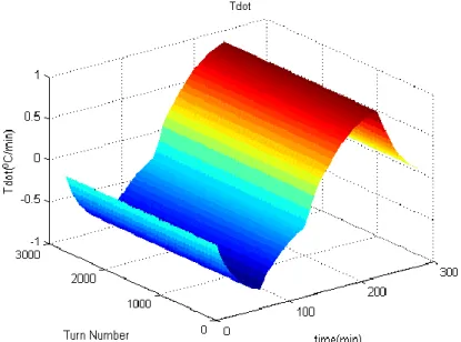
Temperature and the derivative of the temperature of each fiber turn through the coil are given in Figure 3.9 and Figure 3.10. The gradient along the fiber coil is much slower than the derivative with respect to time. In other words, the temperature is diffused through the fiber coil faster relative to the temperature change. This phenomenon supports the layer by layer integration approximation for the Shupe error calculation made by Reference [32].
35
Figure 3.9: Temperature distribution through the fiber coil.
Figure 3.10: Temperature derivative distribution through the fiber coil.
Stress is a disturbance with the components on three directions: Radial, axial, and propagation axis. Stress distributions show different characteristics than the temperature (Figure 3.11, Figure 3.12, and Figure 3.13). Distributions are
36
inhomogeneous which may result in higher bias error than the homogeneous temperature field. Stress gradients are high relative to the time derivative and the graphs get sharper at the edges of the coil.
Figure 3.11: Stress distribution through the coil radial axis.
37
Figure 3.13: Stress distribution through the coil axial axis.
Lastly, bias error estimations are calculated and given with respect to coil temperature in Figure 3.14. Coil temperature starts to decrease from the room temperature to -35°C and turns to increase up to +55°C. Fiber coil visits the temperatures below room temperature twice. Bias error is negative while decreasing and vice versa during the increase phase. This is the effect of the temperature derivative which is aligned with the theory. The Shupe error is nearly twice the elastooptic error. They have the same sign and adds up.
38
Figure 3.14: Bias error estimations vs the coil temperature.
A comparison of the bias error estimations is given in Figure 3.15. Bias errors are in the same order of magnitude, have the same sign, and trends are similar. Bias error of the reference model rapidly goes to a steady point while our model does not. This is due to the slower diffusion of the temperature for our model. The relatively slow temperature diffusion results in greater derivative and gradient for the temperature field.
Figure 3.15: Bias error estimations. Reference [38] (left) and the simulation (right).
-40 -30 -20 -10 0 10 20 30 40 50 60 -0.03 -0.02 -0.01 0 0.01 0.02 0.03
0.04 bias error Shupe
bi as ( o/h ) Temp average (oC) Shupe Elastooptic Total
39
3.3 Advanced Modeling of the Fiber Coil
Classical modeling approaches give insight and valuable conclusions; however, an advanced model is needed for further analysis. We improved the model in two manners: Detailed thermo-mechanical interactions, and the definition of the winding pattern.
Latest approaches in the literature provide more reliable models [14], [39], [40], [41]. The fiber coil is modeled in two steps. The first one is the modeling of the representative volume element (RVE) of the fiber coil by the homogenization process. RVE includes the fiber core, cladding, coating, and adhesive. The second step is the combined model of the homogenous fiber coil defined by the RVE parameters, together with the spool and all other surrounding elements. This two-step approach provide much higher mesh resolutions for the boundaries inside the fiber while running the simulation long enough for thermal diffusion.
Secondly, trimming of the fiber coil is investigated. Quadrupole winding is used for reducing the thermal effects inside the fiber coil. However, the reduction may be decreased if the position of the midpoint of the fiber coil is changed from the ideal case. Midpoint position may shift during the winding of the fiber coil or splicing the phase modulator to the ends of the coil. That shift should be trimmed by shortening the one end of the fiber coil for better performance.
Thirdly, the definition of the quadrupole fiber coil is revised. The practical quadrupole is presented for a better representation of the fiber turn locations. The practical quadrupole is a practical solution for passing the fiber from a layer to the next one. It results in a non-ideal pattern of the quadrupole coil but eliminates the uncontrolled fiber portions between the layers. The pattern also includes the turn length difference between the layers. The model is validated by comparing the simulation results with a laboratory FOG setup.
40
3.3.1 Homogenization / Dehomogenization Procedure
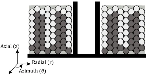
Fiber coil consists of fiber turns, potting material between the turns, and a spool. Fiber itself consists of the core, cladding, and coating. Fiber coil structure, excluding the spool, is an anisotropic, but transversely isotropic composite material (Figure 3.16). The analysis is extended to the composite model for the temperature and stress field formations.
Figure 3.16: Fiber coil is a transversely isotropic composite material [39].
Figure 3.17: Fiber coil RVE. Fibers are located in an orthocyclic manner with adhesive in between. All dimensions are in µm.
Modeling of the whole fiber coil consists of two main steps. Fiber coil is taken as a composite material which is composed of the fiber core, cladding, coating, and adhesive material (Figure 3.17). A model of RVE is simulated (Figure 3.18) to identify the composite material properties. Simulation solves the composite material
41
properties for an orthotropic homogeneous material by using the boundary conditions. A property set (Young’s modulus, Poisson’s ratio, thermal expansion coefficient, all in two dimensions, radial and axial) of an orthotropic homogeneous material representing the fiber coil is obtained. This first step is named homogenization.
Figure 3.18: Simulation of RVE with high resolution meshed.
FEM simulation is reduced to three components, after the homogenization process: Fiber coil as an anisotropic composite material, spool as a homogeneous metal, and air as the surrounding environment. Temperature, stress, and strain fields are obtained by using FEM simulation. These macro-scale fields represent the thermo-mechanical interactions inside and between the spool, fiber coil and environment.
42
The dehomogenization process is carried, after obtaining macro-scale fields. In this process, macro strain fields are mapped to the micro fields. Temperature fields and strain fields at the macro-level results as radial and axial strains inside the fiber. These micro-level strains are used to calculate the bias error calculations.
(𝜀̅𝜀̅𝑟,𝐹 𝑧,𝐹) = ( 𝑀𝑟𝑥 𝑀𝑟𝑦 𝑀𝑟𝑧 𝑀𝑟𝑇 0 0 1 0 ) ( 𝜀̅𝑥𝑥 𝜀̅𝑦𝑦 𝜀̅𝑧𝑧 ∆𝑇 ) (3.26)
where 𝜀̅𝑟,𝐹 and 𝜀̅𝑧,𝐹, are the radial and axial strain fields inside the fiber,
𝑀𝑟𝑥, 𝑀𝑟𝑦, 𝑀𝑟𝑧, 𝑀𝑟𝑇, are the transformation matrix elements,
and 𝜀̅𝑥𝑥, 𝜀̅𝑦𝑦, 𝜀̅𝑧𝑧, are the macro-level strain fields in x, y, z axis respectively.
3.3.2 Coil Winding Pattern
Today, quadrupole and octupole patterns are the most widely used winding methods for tactical and higher grade FOGs. Quadrupole pattern is faster, easier to apply, and provides sufficient performance for many applications. On the other hand, the octupole pattern promises better performance in theory. However, the winding procedure must be undertaken carefully to prevent any non-homogeneity created during the winding.
FEM simulation provides the temperature and stress fields for each fiber turn and time step. Bias error is calculated by using the fields as given in Equation (3.21). In the equation, the parameter ‘z’ defines each turn’s distance from the one end of the fiber loop so that each turn’s location in two-dimensional plane must be specified for any type of winding geometry. A quadrupole pattern is given in Figure 3.7. Fiber turns are located in an orthocyclic manner, by which the fiber turns of each layer is located as close as possible to the next layer. This reduces the distance between the locations of the symmetric fiber portions and provides better thermal performance.
43
Passing the fiber from one layer to the next one, especially from the first layer to the fourth or from the third to the sixth, can be problematic in this pattern. Uncontrolled fiber segments, which are highly susceptible to thermal variations, between the layers exist. This issue can be solved by the practical quadrupole winding pattern (Figure 3.19). The first turn of each layer is wound either CW or CCW and the last turn vice versa. This practical solution for passing the fiber from one layer to the next one changes the locations of the fibers and creates an asymmetry in the axial direction of the coil.
All coil geometry calculations include turn length asymmetry and diameter asymmetry. These asymmetries arise from winding the fiber turns on top of each other. Inner layer turns are shorter and upper ones longer. Innermost and outermost layers have the length difference of (D-d)/π. This length difference changes the error equations in two manners. Firstly, the counter-propagating waves always travel in different layers of the coil, mostly in the next layer. That reduces the quadrupole performance. Secondly, as the Sagnac scale factor is a linear combination of the fiber length and the coil diameter, each layer’s contribution to the bias shift is different from the other. The outermost layers are more sensitive to the rotation rate while the innermost layers less. That phenomenon is also added to the bias error calculation approach.
44
Figure 3.19: Practical Quadrupole Pattern.
3.3.3 Bias Error Calculation Approach
Equation (3.10) is discretized for the calculation of the bias error. The fiber coil is a cylindrical structure and the integral can be represented in radius, azimuth, and height (r,θ,z). Light travels only in the fiber core so that the integral is taken through the fiber core that is only continuous through the azimuth and discrete for axial and radial directions. Equation (3.10) is reduced into two dimensions and discretized.
Ω𝑆(𝑡) = 𝑛 𝜋𝑁∑ 1 𝑑𝑖2∑ ∫ 𝜕𝑛 𝜕𝑇𝑇̇(𝑟𝑖, 𝜃, 𝑧𝑗, 𝑡)(𝐿 − 2𝑠)𝑑𝜃 2𝜋 0 ∆𝑠 𝑁𝑎 𝑗=1 𝑁𝑟 𝑖=1 (3.27)
where 𝑑𝑖 is the diameter of each turn, 𝑁𝑟, 𝑁𝑎 are the radial and axial layer numbers, respectively, and 𝑁 = 𝑁𝑟× 𝑁𝑎 is the total number of turns. Using the relation ∆𝑠 = 𝐿
𝑁= 𝜋𝑑𝑖𝑁
45 Ω𝑆(𝑡) = 𝑛 𝑁∑ 1 𝑑𝑖∑ 𝜕𝑛 𝜕𝑇𝑇̇(𝑟𝑖, 𝑧𝑗, 𝑡)(𝐿 − 2𝑠 − 𝑙𝑖) 𝑁𝑎 𝑗=1 𝑁𝑟 𝑖=1 (3.28)
where 𝑙𝑖 is the length of each fiber turn that is different for every radial layer. This equation is the two-dimensional approximation for the calculation of the bias error due to temperature fluctuation.
3.3.4 Simulations and Results of the Advanced Model 3.3.4.1 Modeling of a Laboratory FOG Coil
A laboratory FOG coil proposed to be navigation grade with 9 cm diameter and 1100 meter length (Table 3.4) is modeled. FEM simulation is built for obtaining the temperature and strain fields. The model consists of the homogenized fiber coil which is wound on a spool, air surrounding the coil, and heat source encapsulating the air (Figure 3.20). Heat source provides a temperature profile ranging from -40 °C to 60 °C. FEM simulation calculates the heat flow according to the material properties of the spool and coil.
46
Figure 3.20: FEM model of the fiber coil.
Table 3.4: Coil parameters
Fiber length (m) 1101
Number of winding layer 36
Number of loops per layer 106
Inner diameter of the coil (mm) 87.00 Outer diameter of the coil (mm) 97.65
Coil height (mm) 18.02
Fiber coil structure is homogenized by defining RVE and calculating the composite material properties by using the boundary conditions as described in Part 3.3.1. Calculated parameters for the design are given in Table 3.5.
47
Table 3.5: Coil parameters obtained by homogenization
Parameter Direction Value
Elastic moduli 𝐸𝑧 (GPa) 14.5 𝐸𝑟 (MPa) 95.2 𝐺𝑧𝑟 (MPa) 24.1 Poisson’s ratio 𝜈𝑧𝑟 0.392 𝜈𝑟 0.979 𝜈𝑟𝑧 0.003 Thermal expansion coefficient 𝛼𝑧 (× 10−6/𝐾) 3.36 𝛼𝑟 (× 10−6/𝐾) 193 Thermal conductivity 𝑘𝑧 (W/mK) 0.51 𝑘𝑟 (W/mK) 0.34
FEM simulation outputs macroscopic temperature and strain fields. Strain fields inside the core are calculated by the dehomogenization process. Transformation matrix elements are obtained along with the homogenization process. Calculated matrix elements are given in Table 3.6.
Table 3.6: Dehomogenization parameters
M𝑟𝑥 2.74 × 10⁻⁶
M𝑟𝑦 2.70 × 10⁻⁶
M𝑟𝑧 -0.17
M𝑟𝑇(1/K) 9.98 × 10⁻⁶
Input temperature profile given in Figure 3.21 spans a range from -40 °C to +60 °C for both increasing and decreasing cases of the temperature. This profile reveals all temperature and temperature time derivative dependent errors in the interval.
48
Figure 3.21: Input temperature profile is obtained from the laboratory experiments.
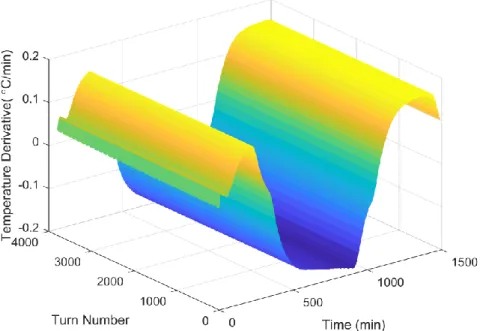
The temperature and derivative of the temperature versus time for each fiber turn through the coil are given in Figure 3.22 and Figure 3.23, respectively. From the graphs, it is seen that the gradient along fiber turns is much slower than the derivative with respect to time. In other words, the temperature is diffused through the fiber coil much faster than the temperature change for this scenario.
0 200 400 600 800 1000 1200 1400 1600 1800 2000 -40 -30 -20 -10 0 10 20 30 40 50 60 Temperature Profile time(min) T( oC)
49
Figure 3.22: Temperature distribution through the fiber coil.
50
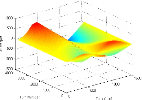
Microscopic strain fields obtained after the dehomogenization are given in Figure 3.24 and Figure 3.25. The time derivatives of the fields are used in the calculation of the elastooptical bias error. From the figures, it can be seen that the stress distribution differs from the temperature distribution, that the gradient in the stress is higher than the time derivative.
51
Figure 3.25: Strain (axial) distribution through the fiber coil.
![Figure 3.5: Steps in the winding of a quadrupole coil [44].](https://thumb-eu.123doks.com/thumbv2/9libnet/5733646.115126/41.918.198.744.174.588/figure-steps-winding-quadrupole-coil.webp)