Galerkin Method for Numerical Solution of Two Dimensional Hyperbolic Boundary Value Problem with Dirichlet Conditions

(1)

Araştırma Araz&Durur/Kırklareli University Journal of Engineering and Science 4-1(2018) 1-11

GALERKIN METHOD FOR NUMERICAL SOLUTION OF TWO

DIMENSIONAL HYPERBOLIC BOUNDARY VALUE PROBLEM WITH

DIRICHLET CONDITIONS

Seda ĠĞRET ARAZ1*_{, Hülya DURUR}2

1*

Siirt University, Faculty of Mathematic Education, 56100, Siirt, TURKEY

2

Ardahan University, Faculty of Engineering, Computer Engineering, 75000, Ardahan, TURKEY

ABSTRACT

In this paper, our aim has been to deal with numerical solution of two dimensional hyperbolic boundary value problem. By applying Galerkin method for solution of this problem, numerical results are obtained and these results are compared with analytical solutions.

Keywords: Hyperbolic Boundary Value Problem, Numerical Approximation, Galerkin Method.

DIRICHLET KOŞULUNA SAHİP İKİ BOYUTLU HİPERBOLİK SINIR

DEĞER PROBLEMİNİN NÜMERİK ÇÖZÜMÜ İÇİN GALERKİN

METODU

ÖZET

Bu çalıĢmada, amacımız iki boyutlu hiperbolik sınır değer probleminin nümerik çözümü ile ilgilenmektir. Bu problemin çözümü için Galerkin metodu uygulanarak nümerik sonuçlar elde edilir ve bu sonuçlar analitik çözümler ile karĢılaĢtırılır.

(2)

1. Introduction and Statement of the Problem

Hyperbolic boundary value problems have been appeared as mathematical modelling of physical phenomena like small vibration of a string, in the fields of science and engineering. In recent years, there has been much attention to studies related with these problems [1, 2, 3].

In this paper, on the domain   _t 

 

0,T where 

   

0,l₁  0,l₂ , we consider

 

x

 

x, , x ,

 

0, tt u   u q uF t  t T (1)

 

x, 0

   

x , _t x, 0

 

x , x u  u   (2)

 

x, 0,



0,



u t _  t T (3) hyperbolic initial-boundary value problem and this problem states wave equation in physical

meaning. 2 2 2 2 x y      _  _  

 is the Laplace operator and



is the boundary of . Also the initial displacement 

 

x and the initial velocity 

 

x are given.

Let us refer from some notations used in this paper.

The space L₂

 

_t is the set of all square integrable functions on the domain  . The Hilbert space called H1

 

_t is the set of functions taken from L₂

 

_t to the spatial variables and time variable of first order. The space

 

o 1

t

H  which is subspace of the space H1

 

_t consists of the functions vanishing at boundary of the domain .

The paper is organized as follows: In section 2, we obtain the generalized solution for hyperbolic problem. In section 3, we refer from the considered numerical method. In section 4, we give three examples and calculate their error norm on the space L₂.

2. Solvability of the Problem

Let us write a priori estimate utilizing energy method to demonstrate the existence, uniqueness and continuity of the solution according to input data[4].

Definition 1. The generalized solution of the problem (1)-(3) is the function

 

o 1

t

uH  and it satisfies the following integral equality;

(3)

 



. x



x

  

x x, 0 x



   

x, x, x t t t t u u q u d dt d F t t d dt                



(4) for all

 

o 1 x,t H t    ,



x,T



0 [5].

Theorem 1. Generalized solution of the problem (1)-(3) in the sense of (4) is exist, unique under

conditions q

 

x L_

 

 ,F

 

x,t L₂

 

_t ,

 

x L₂

 

 ,

 

x H1

 

 and satisfies the following inequality;  



     



1 1 2 2 2 2 2 2 0 t t H L L H u _ c F _   _   _ . (5)

Proof: Multiplying the equation (3) with the function u_t and integrating on the domain and taking into account the condition (3), we write the following inequality;

 







 



   







 





 



   





 

2 2 2 2 2 2 1 1 x, x, x x, x x, 0 x, 0 x x, 0 x 2 2 x, x t t t u t u t q u t d u u q u d F t u d dt     _{ } _  _  _{ } _      



(6)

Let us define the integral J t called energy norm as follows;

 



 





 



   





1/ 2 2 2 2 1 : : x, x, x x, x 2 t J J t u u t u t q u t d     _ _   _ _    _ _   





From energy norm, equality (6) is reorganized like this;

 

 

2 2 0 x, t x 0, J t J F t u d dt t T   

_

 . (7)

Corollary 1. For the problem (1) – (3), the following inequalities are valid;

 

 

2 1 2 , 0, L u J t t T q    (8)  

 

 

2 2 , 0, L u _ J t t T    (9)  

 

 

2 2 , 0, . t L u _  J t t T (10)

By taking derivative of the inequality (7) for t0and applying Cauchy-Bunyakovski inequality, it follows that

(4)

 



 

_{ }



 

2 1 0 x, 0, 2 L t J t  J  F t _ t T (11) If we regulate the equality (11) and take as c₂ max 1,

 

q₂ , we write inequality

 



 

_{ }

 

_{ }

 

_{ }



2 2 2 2 0 x, 0 x, 0 x, 0 2 t L L L c J  u _  u _  u _ . (12)

Using the inequalities (8) and (11), (12), we obtain the following inequality;

 

_{ }



 

_{ }

 

_{ }

 

_{ }

 

_{ }



 

2 2 2 2 2 2 ₂ 2 2 2 2 1 3 , x, 0 x, 0 x, 0 2 x, , 0, 2 t t L L L L L c u t u u u F t t T q              (13)

and from the inequalities (9) and (11), (12), we write

 

_{ }



 

_{ }

 

_{ }

 

_{ }

 

_{ }



 

2 2 2 2 2 2 2 2 2 2 2 , 3 x, 0 x, 0 x, 0 2 x, , 0, t t L L L L L u t _ c u _ u _ u _ F t _ t T          . (14)

However, benefitting from the inequalities (10) and (11), (12) we formulate as follows;

 

_{ }



 

_{ }

 

_{ }

 

_{ }

 

_{ }



 

2 2 2 2 2 2 2 2 2 2 2 , 3 x, 0 x, 0 x, 0 2 x, , 0, t t _L _L t _L _L _L u t _  c u _  u _  u _  F t _  t T . (15)

Summing the inequalities (13), (14) and (15) and after some manipulations, we get the inequality,

 

1_{ }



_{ } _{ } _{ } _{ }



 

2 2 2 2 2 2 2 2 2 3 , _L _L _L _L , 0, H u t _ c F _   _   _   _  t T (16) where ₃ ₂ 2 2 ₂ 1 1 3 3 max 3 , , , 6 2 c c c c c q q    _ _  and

 

1_{ }



_{ } 1_{ } _{ }



2 2 2 2 2 2 4 4 3 , _L _H _L , H u t _ c F _   _   _ c c T . (17)

3. Numerical Solution: Galerkin Method

In this section, we give information about Galerkin method. Galerkin methods have been utilized to solve the problems encountered structural mechanics, dynamics, fluid flow, heat and mass transfer, acoustics, microwave theory, neutron transport, etc. The Galerkin method can be thought of as the calculus of variations performed backwards. That is, the Galerkin method seeks to find the weak form expressed in terms of integrals, and solve that, instead of solving the strong form of the problem as a differential equation.

Galerkin method is an influential numerical method for solving different types of partial differential equations [6, 7, 8]. SubaĢı et al. [9] have applied the Galerkin method to the problem

(5)

of vibration of one dimensional system with free end conditions. Limaco et al. analyzed from the mathematical point of view a model for small vertical vibrations of an elastic string with fixed ends and the density of the material being not constant [10]. The basic Galerkin methods with piecewise linear basis functions and quadratic basis functions have been compared in [11].

In literature, there have been many researches about Galerkin method which is an important tool in for numerical solution of hyperbolic problems [12, 13, 14].

The main contribution of this study is to obtain a successful approximation for two dimensional hyperbolic boundary value problem with variable coefficient. The proposed method has been improved to solve equations with transverse elastic force which is the function q

 

x taken place in the coefficient of hyperbolic problem.

Now, we apply this method to the considered problem.

By using Galerkin Method, the approximate solutions for the problem (1)-(3) are written as follows;

 

   

1 1 x, x N N N N ij ij i j u t c t v   



where the coefficients c_ijN

 

t are the functions such that

 

   

_{ } 2 x, , x N N ij ij _L c t  u t v _

fori j, 1, 2,...,N and the functions v_ij

 

x are basis functions for which

   

  2 x , x ij ij kl _L kl v v  

is valid for k l, 1, 2,...,N. Here _klij is Kronecker delta. Let us write the equation (1) for the approximations uN

 

x,t so that we obtain the coefficients c_ijN

 

t

   

 

   

 

2 2 1 1 1 1 1 1 x x x x, N N N N N N N ij N N ij ij ij ij ij i j i j i j d c t v c t v q x c t v F t dt          



(19)

and then integrate on the domain  after multiplying both side of equality (19) with the function

 

x

kl

(6)

   

     

   

2 2 1 1 1 1 1 1 x x x x x x, x x N N N N N N N ij N N ij ij ij ij ij kl kl i j i j i j d c t v c t v q x c t v v d F t v d dt                   







(20) where

   

  2 x , x 0 ij kl _L v v _  and

   

  2 x , x 0 ij kl _L v v _   as

   

i j,  k l, . Let us we write this system in the matrix form of

 

   

 

2 2 0 , 0 N N N N d C t V t C t F t dt d C D C E dt     (21)

whereCN

 

t is the matrix of searched functions that is,

 

11 12 1 21 22 2 1 2 N N N N N N N N N N N N N N NN c t c t c t c t c t c t C t c t c t c t                (22)

and the coefficient matrix V t defined by

 

       

_{ }

     

 

_{ }

     

 

_{ }

     

 

_{ } 2 2 2 2 11 11 11 1 1 1 1 1 1 x, x , x x, x , x x, x , x x, x , x N N N L L N N N _L NN NN NN _L v t q x v v v t q x v v V t v t q x v v v t q x v v                 _ _ _ _      . (23)

The right hand side of matrix is in the form of

 

   

_{ }

   

_{ }

 

_{ }

   

_{ }

   

_{ }

 

_{ }

 

_{ }

 

_{ }

 

_{ } 2 2 2 2 2 2 2 2 2 11 12 1 21 22 2 1 2 x, , x x, , x x, , x x, , x x, , x x, , x x, , x x, , x x, , x N L L L N L L L N _L N _L NN _L F t v F t v F t v F t v F t v F t v F t F t v F t v F t v                           . (24)

(7)

 

11 12 1 11 12 1 21 22 2 21 22 2 1 2 1 2 0 0 0 0 0 0 0 0 0 0 0 0 , 0 0 0 0 0 0 N N N N N N N N N N N N N N N N N N N N N NN N N N N N NN d d d c c c dt dt dt c c c d d d c c c c c c D E dt dt dt c c c d d d c c c dt dt dt       _ _   _ _   _ _ _ _      _ _     _ _     (25) subject to

 

   

  2 0 x , x N ij ij _L c v    and

 

   

_{ } 2 0 x , x N ij ij _L d c v dt    .

By calculating the coefficients c_ijN

 

t , we obtain the approximate solutionuN

 

t . The equation (21) states a system of second order ODE and the solution of this system is uniquely solvable.

4. Numerical Illustrations

In this section, we present test problems after giving theoretical information mentioned in the previous sections. Before giving illustrations, we refer from its properties and basis functions which we will use for solving examples. In this article, we take the following fundamental set as basis functions

 





1 2 1 2 1 2 1 2 1 2 1 2 2 2 2

x sin sin ,..., sin sin ,..., sin sin

ij x y i x j y N x N y v l l l l l l l l l l l l                                                   

for which the following statements are hold;



   

_{ }

   

2 0, , , x , x 1, , , ij kl _L i j k l v v i j k l               

   

 

   

2 2 2 1 2 0, , , x , x , , , ij kl _L i j k l v v _i _j i j k l l l          _{ }_ _ _ _ _              .

Example 1. Let us consider problem (1)-(3) on the domain

 

x y, 

   

0, 2  0, 2 and t

 

0,t

where 

 

x y, 0, 

 

x y, 0,

 

 

1 0 and 1, 0, 2 x ₁ 1 and 2, 0, 2 3 x x y q x x y x             

(8)

Araştırma Araz&Durur/Kırklareli University Journal of Engineering and Science 4-1(2018) 1-11 and

 





   





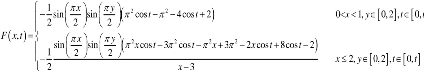
2 2 2 2 2 2 1

sin sin cos 4cos 2 0< 1, 0, 2 , 0,

2 2 2

,

sin sin cos 3 cos 3 2 cos 8cos 2

1 2 2 2, 2 3 x y t t x y t t F x t _x _y x t t x x t t x y x   _ _   _ _ _ _      _ _{ } _            _ _{ } _                  

   

0, 2 ,t 0,t        

In this case, by solving the system (21), the exact solution is equal to approximate solution which

is

 

x,

  

x, 1 cos



sin sin

2 2

N x x

u t u t   t _ _ _ _

   for N 10.

The graphs of these solutions are given in Figure 1.

Approximate Solution Exact Solution Errors for _{ }

2 N L u u _ 0 t 0.0001 2 t 0.0002 4 t 0.0001 6 t 0.0005 8 t 0.00006 10 t 0.0004

Figure 1: The graph of the approximate solution and exact solution forN10, t1.

Example 2. Let us analyze problem (1)-(3) on the domain

 

x y, 

   

0,1  0, 2 and t

 

0,t where 

 

x y, 0, q

 

x x

 





 







 

1 3 1 2 1 sin 0< , 0, 2 2 2 2 , 1 3 1 2 1 sin 1, 0, 2 2 2 y x x x y x y y x x x y     _   _ _             _ _    _ _  and

 





   





   

2 2 2 3 2 2 2 2 3 2 2 1 3 1 cos sin 18 9 8 12 4 16 , 0, 2 , 0, 8 2 2 , 1 3 cos sin 18 27 8 9 20 16 20 1, 0, 2 , 0, 8 2 y t x x x x x x y t t F x t y t x x x x x x y t t  _ _  _ _ _    _ _ _ _ _ _ _ _           _ _           _ _ 

(9)

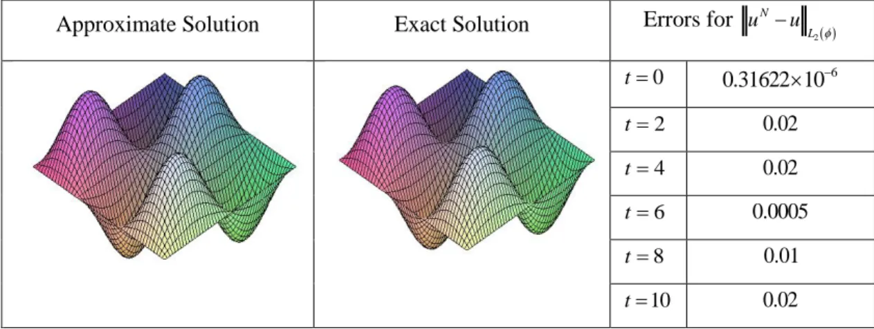
In this case, the exact solution is

 





   







   

1 3 1 2 1 cos sin , 0, 2 , 0, 2 2 2 x, 1 3 1 2 1 cos sin 1, 0, 2 , 0, 2 2 y x x t x y t t u t y x x t x y t t    _   _ _ _             _ _     _ _  .

The graphs of these solutions are given in Figure 2.

2 N L u u _ 0 t _{0.31622 10} 6 2 t 0.02 4 t 0.02 6 t 0.0005 8 t 0.01 10 t 0.02

Figure 2: The Graph of the Approximate Solution and Exact Solution forN10, t1

Example 3. Let us solve problem (1)-(3) on the domain

 

x y, 

   

0,1  0,1 and t

 

0, .t For this example, we shall take as q

 

x  x y, 

 

x y, sinxsiny,

 

x y,  sinxsiny,

 



2



x, tsin sin 2 1

F t e x y    x y

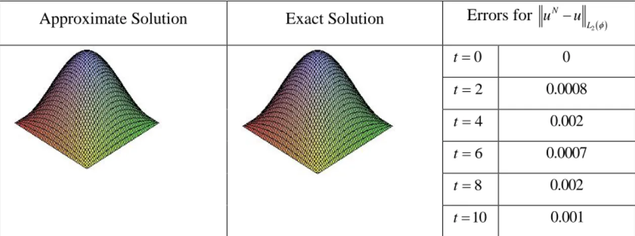
In this case, it can be seen that the exact solution is u

 

x,t etsinxsiny.

(10)

2 N L u u _ 0 t 0 2 t 0.0008 4 t 0.002 6 t 0.0007 8 t 0.002 10 t 0.001

Figure 3: The Graph of the Approximate Solution and Exact Solution forN10, t1

5. Conclusion

In this paper, Galerkin method with basis functions has been proposed to solve two dimensional hyperbolic boundary value problems. The existence, uniqueness and dependence continuously of generalized solution for problem have been demonstrated by Theorem 1. It is considered three illustrations for the hyperbolic boundary value problem in this article.

Speaking for the examples presented, it can be seen that the method is successful. In other words, the numerical results confirm the validity of the technique. It has been utilized from Maple in numerical calculations.

6. References

[1] Ġsmailov M.I., Tekin Ġ., Inverse coefficient problems for a first order hyperbolic system,

Applied Numerical Mathematics, 106, 98-115, 2016.

[2] Zadvan H., Rashidinia J., Non-polynomial spline method for the solution of two-dimensional

linear wave equations with a nonlinear source term, Numerical Algorithms, 1-18, 2016.

[3] Merad A., Vaquero, J.M., A Galerkin method for two dimensional hyperbolic

integro-differential equation with purely integral conditions, Applied Mathematics and Computation, 291, 386-394, 2016.

[4] Hasanov A., Simultaneous determination of the source terms in a linear hyperbolic problem

from the final over determination: weak solution approach, IMA Journal of Applied Mathematics, 74, 1-19, 2008.

(11)

[5] Ladyzhenskaya O.A., Boundary Value Problems in Mathematical Physics, Springer-Verlag,

1985.

[6] Li, Q.H., Wang J., Weak Galerkin Finite Element methods for parabolic equations, Numerical

Methods for Partial Differential Equations, 29,2004-2024, 2013.

[7] Dedner, A., Madhavan P., Stinner B., Analysis of the discontinuous Galerkin method for

elliptic problems on surfaces, IMA Journal of Numerical Analysis, 33, 952-973, 2013.

[8] Huang Y., Li J., Li D., Developing weak Galerkin finite element methods for the wave

equation, Numerical Methods for Partial Differential Equation, 33,3,2017.

[9] SubaĢı M., ġener S.ġ., Saraç Y., A procedure for the Galerkin method for a vibrating system,

Computers and Mathematics with Applications, 61, 2854-2862, 2011.

[10] Límaco J., Clark H.R., Medeiros L.A., Vibrations of elastic string with nonhomogeneous

material, J. Math. Anal. Appl. 344, 806–820, 2008.

[11] Sengupta T.K., Talla S.B., Pradhan S.C., Galerkin finite element methods for wave

problems, Sadhana, 30, 5, 611–623, 2005.

[12] McDonald, M.A., Lamoureux M.P., Margrave G.F., Galerkin methods for numerical

solutions of acoustic, elastic and viscoelastic wave equations, CREWES Research Report, 24, 2012.

[13] J. Suk, Y. Kim, Modeling of vibrating systems using time-domain finite element method, J.

Sound Vib. 254, 3, 503–521, 2002.

[14] Mancuso M., Ubertini F., An efficient time discontinuous Galerkin procedure for non-linear