NON-ABELIAN FUNDAMENTAL GROUP
Alex Degtyarev
Abstract. We calculate the fundamental groups π = π1(P2r B) for all irreducible
plane sextics B ⊂ P2 with simple singularities for which π is known to admit a
dihedral quotient D10. All groups found are shown to be finite, two of them being of
large order: 960 and 21600.
1. Introduction
1.1. Motivation. Recall that a plane sextic B ⊂ P2is said to be of torus type, or tame, if its equation can be represented in the form p3+ q2= 0, where p and q are
some homogeneous polynomials of degree 2 and 3, respectively. Essentially, sextics of torus type were introduced by O. Zariski as the ramification loci of cubic surfaces. The fundamental group π = π1(P2r B) of an irreducible sextic B of torus type
is known to be infinite; in particular, it is nonabelian. For a long time, no other examples of nonabelian groups were known, which lead M. Oka to a conjecture [7] that the fundamental group of an irreducible sextic that is not of torus type is always abelian. The conjecture was disproved in [3], [4], and for the counterexamples for
which the group π was computed it turned out to be finite, with the exception of
one family with non-simple singularities. Besides, it was also shown that, for each irreducible sextic that is not of torus type, the abelinization of the commutant of π is finite. (This assertion is a restatement of the proved part of Oka’s conjecture, related to the Alexander polynomial.) Thus, the following statement seems to be a reasonable replacement for the original conjecture.
1.1.1. Conjecture. Let B be an irreducible plane sextic with simple singularities
and not of torus type. Then the fundamental group π1(P2r B) is finite.
The fundamental groups of all irreducible sextics with a non-simple singular point are found in [3] (the case of a quadruple point) and [4] (the case of a singular point adjacent to J10). On the other hand, the construction of sextics with simple
singularities and nonabelian fundamental group π = π1(P2r C) suggested in [3] is
rather indirect; it proves that π has a dihedral quotient, but it is not suitable to compute π exactly. In this paper, we attempt to substantiate Conjecture 1.1.1 by computing the groups of some of the curves discovered in [3].
2000 Mathematics Subject Classification. Primary: 14H30 Secondary: 14H45.
Key words and phrases. Plane sextic, non-torus sextic, fundamental group, dihedral covering.
Typeset by AMS-TEX 1
1.2. Principal results. For a group G, denote by G0 = [G, G] its commutant, or derived group, and let G00 = (G0)0 etc. We use the notation Z
n and Dn for, respectively, the cyclic and dihedral groups of order n.
To shorten the statements, we introduce the term generalized D2n-sextic to stand
for a plane sextic B whose fundamental group π1(P2r B) factors to D2n, n > 3. A
D2n-sextic is an irreducible generalized D2n-sextic with simple singularities. Recall,
see [3], that there are D6-, D10-, and D14-sextics; all D6-sextics are of torus type,
and the D10-sextics form eight equisingular deformation families, one family for
each of the following sets of singularities:
4A4, 4A4⊕ A1, 4A4⊕ 2A1, 4A4⊕ A2,
A9⊕ 2A4, A9⊕ 2A4⊕ A1, A9⊕ 2A4⊕ A2, 2A9.
The objective of the paper is the computation of the fundamental groups of all D10-sextics. The principal result is the following theorem.
1.2.1. Theorem. Let B be a D10-sextic. Then the group π = π1(P2r B) is finite. Furthermore, one has π = D10⊗ Z3with the following two exceptions:
(1) The set of singularities of B is 4A4⊕ 2A1: then ord π = 960 and one has π00/π000= (Z
2)4 and π000= Z2.
(2) The set of singularities of B is A9⊕ 2A4⊕ A2: then ord π = 21600 and π00 is the only perfect group of order 720, see [9].
(In all cases, including the exceptional ones, π/π0= Z
6 and π0/π00= Z5.)
According to [3], the D14-sextics form two equisingular deformation families,
with the sets of singularities 3A6and 3A6⊕ A1. For the former family, the group
has recently been shown to be D14× Z3, see [6]. The group of the sextics with the
set of singularities 3A6⊕A1(which are all projectively equivalent) is still unknown.
The groups of the D10-sextics with the sets of singularities 4A4 and 4A4⊕ A1
were found independently by C. Eyrol and M. Oka [8].
1.3. Other results and contents. The starting point of the computation is Theorem 2.1.1, which provides an explicit geometric construction for D10-sextics.
(In [3], only the existence of D10-sextics with the sets of singularities listed above is
proven.) We show that each D10-sextic B is a double covering of a very particular
rigid trigonal curve ¯B in the Hirzebruch surface Σ2; the curve ¯B has two type A4
singular points, and various sets of singularities for B are obtained by varying the ramification locus. Theorem 2.1.1 is dealt with in Section 2.
The fundamental groups are computed in Section 3: we merely apply the classical approach due to van Kampen to the ruling of the Hirzebruch surface Σ2. In a few
difficult cases, the resulting representations are studied using GAP.
Section 4 is not directly related to Theorem 1.2.1: we use the representation given by Theorem 2.1.1 to produce explicit equations for D10-sextics. The equation
depends on three parameters a, b, c ∈ C, see (4.2.1); we analyze the parameter space and describe the triples (a, b, c) resulting in particular sets of singularities.
1.4. Acknowledgements. I am thankful to the organizers of the Fourth Franco-Japanese Symposium on Singularities held in Toyama in August, 2007 for their hospitality and for the excellent working conditions. A great deal of time consuming computations used in the paper was done using GAP and Maple, and I am taking this opportunity to extend my gratitude to the creators of these indispensable software packages.
2. The construction
2.1. The reduction. Recall that any involutive automorphism c : P2→ P2has a
fixed line L = Lc and an isolated fixed point O = Oc, and the quotient P2(O)/c is
the rational geometrically ruled surface Σ2. (Here, P2(O) stands for the plane P2
with O blown up.) The images in Σ2of O and L are, respectively, the exceptional
section E and a generic section ¯L, so that P2(O) is the double covering of Σ 2
ramified at ¯L + E.
Recall also that the semigroup of classes of effective divisors on Σ2 is generated
by E and the class F of a fiber of the ruling. One has E2= −2, F2= 0, F ◦ E = 1,
and KΣ2 = −2E − 4F .
The principal result of this section is the following theorem. 2.1.1. Theorem. Let B ⊂ P2 be a D
10-sextic. Then P2 admits an involution c preserving B, so that Oc ∈ B, and the image of B in Σ/ 2= P2(Oc)/c is a trigonal curve ¯B, disjoint from E, with two type A4singular points.
Theorem 2.1.1 is proved at the end of this section, in 2.5 below. Theorem 2.1.1 has a partial converse, see Theorem 3.2.8.
Remark. The proof of Theorem 2.1.1 given in 2.5 uses the theory of K3-surfaces;
we do prove that each D10-sextic is symmetric. The fact that each of the eight
equisingular deformation families of such sextics admits a symmetric representative can easily be established using the results of Section 3, where each set of singularities listed in the introduction is realized by a symmetric D10-sextic.
2.2. The covering K3-surface. Let B be a plane sextic with simple singularities. Consider the double covering X → P2ramified at B and its minimal resolution ˜X.
Then, ˜X is a K3-surface and the deck translation τ : ˜X → ˜X of the covering is a
holomorphic anti-symplectic (i.e., reversing holomorphic 2-forms) involution. Recall that H2( ˜X) ∼= 2E8⊕ 3U is an even unimodular lattice of rank 22 and
signature −16. For a singular point P of B, denote by DP ⊂ H2( ˜X) the set of
classes of exceptional divisors over P ; we use the same notation DPfor the incidence graph of these divisors, which is an irreducible Dynkin diagram of the same name A–D–E as the type of P . Note that, for a type A singular point, the action of τ∗ on DP is the only nontrivial symmetry of the graph. Let ΣP ⊂ H2( ˜X) be the
sublattice spanned by DP; it is an irreducible negative definite root system. Denote Σ =LΣP, the summation running over all singular points P of B, and let S = Σ ⊕ Zh ⊂ H2( ˜X), where h ∈ H2( ˜X) is the class realized by the pull-back
of a generic line in P2. One has h2 = 2, and the sums above are orthogonal. Let
˜
Σ ⊂ ˜S ⊂ H2( ˜X) be the primitive hulls of Σ and S, respectively. The finite index
extension ˜S ⊃ S is determined by its kernel K, which is an isotropic subgroup of
the discriminant group discr S. (For the definition of the discriminant group and its relation to lattice extensions, see V. V. Nikulin [11].) As shown in [2], if B is irreducible, then K ⊂ discr Σ. According to [3], it is the kernel K that essentially enumerates the dihedral quotients of π1(P2r B).
2.3. Symmetric sextics. Let B be a plane sextic with simple singularities, and denote by ˜X the covering K3-surface. Let ˜c: ˜X → ˜X be a holomorphic symplectic
(i.e., preserving holomorphic 2-forms) involution. As is known, ˜c has eight fixed points, and the quotient Y = ˜X0/˜c is again a K3-surface, where ˜X0 is ˜X with the fixed points of ˜c blown up.
Since the projection ˜X → P2is the map defined by the linear system h ∈ Pic ˜X,
the two involutions ˜c, τ commute if and only if the induced automorphism ˜c∗ of
H2( ˜X) preserves h. In this case, ˜c descends to an involution c : P2 → P2 which
preserves B. Let O = Oc and L = Lc. In what follows, we always assume that B
does not contain L as a component. We fix the notation ¯L and ¯B for the images
of L and B, respectively, in Σ2.
Alternatively, if ˜c∗(h) = h, then τ descends to an anti-symplectic involution
τY: Y → Y , and the quotient Y/τY blows down to Σ2.
2.3.1. Lemma. Let O, B, ¯B, etc. be as above. If O /∈ B, then ¯B ∈ |3E + 6F | is a trigonal curve disjoint from E. If O ∈ B, then ¯B ∈ |2E + 6F | is a hyperelliptic curve, ¯B ◦ E = 2.
Proof. The branch locus of the ramified covering Y → Σ2 consists of ¯B, ¯L, and,
if O ∈ B, the exceptional section E. On the other hand, since Y is a K3-surface, the branch locus is an anti-bicanonical curve, i.e., it belongs to |4E + 8F |. Since
¯
L ∈ |E + 2F |, the statement follows. ¤
2.3.2. Lemma. Let P be a c-invariant type Apsingular point of B, and let ¯P ∈ Σ2 be its image. Assume that p > 1 and that ˜c∗acts trivially on DP. Then P ∈ L and
¯
P is a type A2p+1 singular point of ¯B + ¯L, i.e., a point of (p + 1)-fold intersection of ¯L and ¯B at a smooth branch of ¯B. Conversely, the double covering of a curve ¯B as above has a type Ap singular point.
Proof. Since each curve in DP is preserved by ˜c (as a set), the intersection points of the curves must be fixed by ˜c. Furthermore, each of the two outermost curves must contain one more fixed point of ˜c. Blowing up the fixed points, one obtains a sequence of rational curves with the following incidence graph:
c s c s . . . s c s c
(Here, c and s stand, respectively, for (−1)- and (−4)-curves; the vertices in the diagram alternate and their total number is 2p + 1.) The (−1)-curves are in the fixed point set of ˜c, and the (−4)-curves are not. Hence, the projection of the exceptional divisor to Y is a sequence of (2p + 1) rational curves whose incidence graph D is A2p+1. The involution τY induced from τ acts on D as the only nontrivial
symmetry; in particular, it is nontrivial on the middle curve. Thus, the projection to Y/τY is a chain of p (−2)-curves ending in a (−1)-curve; it blows down to a single type A2p+1 singular point of the branch locus.
The converse statement can be proved by analyzing a local equation of ¯B + ¯L,
so that ¯L = {y = 0}, and substituting y 7→ y2. ¤
2.3.3. Lemma. Let P be a c-invariant type Apsingular point of B, and let ¯P ∈ Σ2 be its image. Assume that either p = 1 or p > 1 and ˜c∗ acts nontrivially on DP.
Then p = 2k − 1 is odd and either
(1) P ∈ L and ¯P is a type Dk+2 (type A3 if p = 1) singular point of ¯B + ¯L, or
(2) P = O and ¯P is a type Dk+1 singular point (a pair of type A1 singular points if p = 1) of ¯B + E.
The type Ds singular point above is formed by the section ¯L or E intersecting ¯B
with multiplicity 2 at a type As−3 singular point of ¯B. Conversely, the double
Proof. If p were even, the two middle curves in the exceptional divisor over P would
intersect transversally at a fixed point of ˜c. Since ˜c is symplectic, it cannot trans-pose two such curves. (The differential d˜c at each fixed point is the multiplication by (−1).) Hence, p is odd.
The middle curve in the exceptional divisor is fixed by ˜c; hence, it contains two fixed points. Blowing them up, one obtains a collection of rational curves with the following incidence graph:
c
.c . . . .c s .c . . . .c c
(Here, c, .c, and s stand, respectively, for (−1)-, (−2)-, and (−4)-curves; the total number of curves is p + 2 = 2k + 1, the action of ˜c∗ on the graph is the horizontal symmetry, and ˜c fixes the two (−1)-curves pointwise.) The projection of this divisor to Y is a collection of (k + 2) rational curves whose incidence graph is Dk+2(the ‘short’ edges corresponding to the two (−1)-curves in ˜X).
Since τY is anti-symplectic, whenever two invariant curves intersect transversally at a fixed point, exactly one of them is fixed by τY pointwise. Hence, the action of τY on the exceptional divisor is determined by its action on the curve with three neighbors in the incidence graph. Depending on whether this action is trivial or not, the projection of the exceptional divisor to Y/τY has one of the following two incidence graphs:
c
s c s . . . c
or .c c s c . . .
Now, depending on the parity of k, these graphs blow down either to a single type Dk+2 singular point of the branch locus (if the last vertex corresponds to a (−1)-curve) or to a (−2)-curve with a type Dk+1 singular point on it (if the last vertex corresponds to a (−4)-curve); in the latter case, the remaining (−2)-curve is the exceptional section E ⊂ Σ2.
The converse statement is proved by analyzing a local equation. ¤
For completeness, we also consider the case of type D and E singular points. 2.3.4. Lemma. Let P be a c-invariant singular point of B of type D or E, and
let ¯P ∈ Σ2 be its image. Then ˜c∗ acts nontrivially on DP; in particular, P is of
type Dq, q > 4, or E6. Furthermore, P ∈ L and ¯P is, respectively, a type D2q−2 or E7 singular point of ¯B + ¯L; in the former case, ¯P is a simple node of ¯B with one of the branches tangent to ¯L. Conversely, the double covering of a curve ¯B as above has a corresponding type Dq or E6 singular point.
Proof. If ˜c∗ acted trivially on DP, then the curve with three neighbors in the diagram would have three fixed points and thus it would be fixed by ˜c. Hence, the action is nontrivial. This observation rules out type E7 and E8 singular points.
The further analysis is completely similar to the proof of Lemma 2.3.3, with the additional simplification that the diagram in Y is asymmetric and, hence, the curve with three neighbors is fixed by cY. We omit the details. ¤
2.4. Construction of the involution. All D10-sextics are described in [3]; any
such curve has ‘essential’ set of singularities 4A4, A9⊕ 2A4, or 2A9plus, possibly,
a few other singular points of type A1or A2.
Let B be a D10-sextic. Pick a point P = Pi of type A4 (respectively, a point P = Qk of type A9), choose an orientation of its (linear) graph DP, and denote by ei1, . . . , ei4(respectively, fk1, . . . , fk9) the vertices of DP, numbered consecutively according to the chosen orientation. Let e∗
ij (respectively, fkj∗) be the dual basis for Σ∗
P ⊂ ΣP ⊗ Q. Note that e∗ij = −ei,5−j∗ mod ΣP and fij∗ = −fi,10−j∗ mod ΣP. According to [3], under an appropriate numbering of the singular points and appropriate orientation of their graphs DP, the kernel K of the extension ˜Σ ⊃ Σ is the cyclic group Z5 generated by the residue γ = ¯γ mod Σ, where ¯γ is given by
e∗
11+ e∗21+ e∗32+ e∗42, f14∗ + e∗11+ e∗21, or f14∗ + f22∗
(for the set of essential singularities 4A4, A9⊕ 2A4, or 2A9, respectively).
Define an involution cS: S → S as follows: – h 7→ h,
– x 7→ x for x ∈ ΣP for P a singular point other than A4or A9,
– e1j ↔ e2,5−j, e3j↔ e4,5−j, j = 1, . . . , 4,
– fkj↔ fk,10−j, j = 1, . . . , 9.
It is immediate that cS acts identically on the p-primary part of discr S for any prime p 6= 5, and the action of cS on the 5-primary part discr S ⊗ F5 (which can
be regarded as an F5-vector space) has two dimensional (−1)-eigenspace which
contains K as a maximal isotropic subgroup, so that K⊥/K can be identified with the (+1)-eigenspace of cS. Hence, cS extends to an involution ˜cS: ˜S → ˜S, the latter
acts identically on discr ˜S, and the direct sum ˜cS⊕ idS⊥ extends to an involution
˜c∗: H2(X) → H2(X).
By construction, ˜c∗preserves h and, since it acts identically on the transcendental lattice (Pic X)⊥ ⊂ ˜S⊥, it also preserves classes of holomorphic forms. Furthermore, ˜c∗ preserves the positive cone of X. (Recall that the positive cone is an open fundamental polyhedron V+ ⊂ (Pic X) ⊗ R of the group generated by reflections
defined by vectors x ∈ Pic X with x2 = −2; it is uniquely characterized by the
requirement that V+ · e > 0 for any exceptional divisor e ∈ S
PDP and that the closure of V+ should contain h.) Due to the description of the fine period
space of marked K3-surfaces given in A. Beauville [1], ˜c∗ is induced by a unique involutive automorphism ˜c: X → X, which is symplectic and commutes with the deck translation τ . The descent of ˜c to P2is the involution c the existence of which
is asserted by Theorem 2.1.1.
2.5. Proof of Theorem 2.1.1. The involution c : P2→ P2 is constructed in 2.4.
Due to Lemmas 2.3.1–2.3.3 (and the description of the singularities of B and the action of ˜c∗on the set of exceptional divisors, see 2.4), the image ¯B ⊂ Σ2is either a
trigonal curve with the set of singularities 2A4(and then O /∈ B) or a hyperelliptic
curve with the set of singularities 2A4 or A4⊕ A3. The latter possibility is ruled
out by the fact that the genus of a nonsingular curve in |2E + 6F | is 3. ¤ 3. Calculation of the groups
3.1. The curve ¯B. The trigonal curve ¯B ⊂ Σ2 with two type A4 singular points
a curve is unique; its skeleton Sk ⊂ P1 (see [5]) is shown in Figure 1. One can
observe that the skeleton is symmetric with respect to the dotted grey line (the real structure z 7→ ¯z on P1) and, properly drown, it is also symmetric with respect
to the holomorphic involution z 7→ −1/z. Hence, the curve ¯B can be chosen real
and symmetric with respect to a real holomorphic involution of Σ2 (see Section 4
below for explicit equations). Furthermore, all singular fibers of ¯B (two cusps and
two vertical tangents) are also real.
Figure 1. The skeleton of ¯B
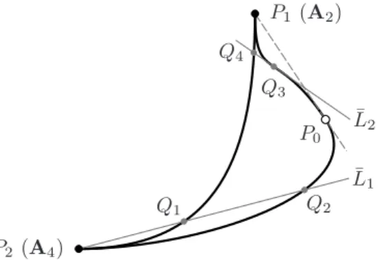
Alternatively, ¯B can be obtained as a birational transform of a plane quartic C
with the set of singularities A4⊕ A2, see Figure 2. (Up to automorphism of P2,
such a quartic is also unique.) In the figure, the line (P0P1) is tangent to C at P0,
and the transformation consists in blowing P0 up twice and blowing down the
transform of (P0P1) and one of the exceptional divisors over P0. Lines through P0
other than (P0P1) transform to fibers of Σ2; this observation gives one a fairly good
understanding of the geometry of ¯B, see, e.g., Figure 4.
¯ L1 Q1 Q2 ¯ L2 Q3 Q4 P1(A2) P2 (A4) P0
Figure 2. The quartic C with the set of singularities A4⊕ A2
3.2. Van Kampen’s method. To calculate the fundamental group, we fix a real curve ¯B as in 3.1 and choose an appropriate real section ¯L intersecting ¯B at real
points. Let F1, . . . , Fk be the singular fibers of ¯B + ¯L (i.e., the fibers intersecting ¯
B + ¯L at less than four points). Under the assumptions, they are all real. In the
figures below, the curves ¯B and ¯L are shown, respectively, in black and grey, and
the singular fibers are the vertical grey dotted lines.
Fix a real nonsingular fiber F∞intersecting ¯B at one real point, and consider the affine part Σ2r(E∪F∞), cf. Figure 4. Pick a real nonsingular fiber F intersecting ¯B
at three real points and a generic real section S. We identify S with the base of the ruling. Let x = S ∩ F , x∞= S ∩ F∞, and xi= S ∩ Fi, i = 1, . . . , k. Assume that S is proper in the following sense: there is a segment I ⊂ SRcontaining x and all xi,
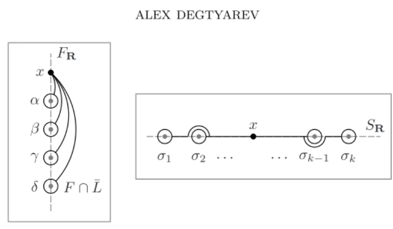
FR α β γ δ F ∩ ¯L x SR σ2 σ1 . . . σk−1 σk x
Figure 3. The basis α, β, γ, δ and the loops σi
i = 1, . . . , k, and disjoint from ¯B and ¯L. (The usual compactness argument shows
that such a section exists.) In the figures, we assume that I lies above ¯B and ¯L.
Let G = π1(F r ( ¯B ∪ E ∪ ¯L), x), and let α, β, γ, δ be the basis for G shown
in Figure 3, left. (All loops are oriented in the counterclockwise direction.) We
always assume that δ is a loop around F ∩ ¯L. (Sometimes, the generators should
be reordered by inserting δ between α and β or β and γ, cf. 3.3 and 3.4. In these cases, we show that δ commutes with all subsequent generators, so that the reordering is irrelevant.) Let, further, σ1, . . . , σk be the basis for the group
π1(Sr{x1, . . . , xkx∞}, x) shown in Figure 3, right: each σiis a small circle about xi connected to x by a real segment li ⊂ SR bent to circumvent the other singular
fibers in the counterclockwise direction.
3.2.1. Definition. The braid monodromy along a loop σi, i = 1, . . . , k, is the automorphism mi: G → G resulting from dragging F along σi while keeping the base point in S. (Since S is proper, miis indeed a braid.)
3.2.2. Proposition. The group Π = π1(Σ2r ( ¯B ∪ E ∪ ¯L)) is given by
(3.2.3) Π =α, β, γ, δ¯¯ mi= id, i = 1, . . . , k, (αβγδ)2= 1®,
where each braid relation mi= id should be understood as a quadruple of relations
mi(α) = α, mi(β) = β, mi(γ) = γ, mi(δ) = δ.
Proof. The representation (3.2.3) is the essence of van Kampen’s method, see [10],
applied to the ruling of Σ2. The only statement that needs proof is the last relation
(αβγδ)2= 1, resulting from the patching of the fiber at infinity F∞. This relation
is [∂D] = 1, where D ⊂ S is a small disk around F∞∩ S. If the base fiber F is
sufficiently close to F∞, then [∂D] = (αβγδ)2, as in this case one can take for S a
small perturbation of E +2F . In general, due to the properness of S, the translation homomorphism between any two nonsingular fibers is a braid; hence, it leaves the product αβγδ invariant and the relation has the same form for any fiber F . ¤
In sections 3.3–3.6 below, we attempt to calculate Π using Proposition 3.2.2. To find the braid monodromy mi, we represent it as the local braid monodromy along a small circle surrounding xi, conjugated by the translation homomorphism along the real path li connecting xi to x. The former is well known: it can be found by considering model equations. For the latter, we choose the models so that, at each
moment, all but at most two points of the curve are real; in this case, the resulting braids are written down directly from the pictures.
The following lemma facilitates the calculation by reducing the number of fibers to be considered.
3.2.4. Lemma. In representation (3.2.3), (any) one of the braid relations mi= id
can be ignored.
Proof. The product σ1. . . σk is the class of a large circle encompassing all singular fibers. Hence, mk◦ . . . ◦ m1is the so called monodromy at infinity, which is known
to be the conjugation by (αβγδ)2. In view of the last relation in (3.2.3), each mi
is a composition of the others. ¤
For the rest of this section, we fix the notation α, β, γ, δ for generators of the group Π = π1(Σ2r ( ¯B ∪ E ∪ ¯L)), chosen as explained above. The generator δ plays
a special rˆole in the passage to π = π1(P2r B).
3.2.5. Proposition. The fundamental group π = π1(P2r B) is the kernel of the homomorphism Π/δ2→ Z
2, α, β, γ 7→ 0, δ 7→ 1.
Proof. The statement is a direct consequence of the construction: one considers the
appropriate double covering of Σ2r ( ¯B ∪ E ∪ ¯L) and patches L. ¤
3.2.6. Lemma. If δ is a central element of Π/δ2, then π
1(P2r B) = D10× Z3. Proof. Since δ is a central element, the relation (αβγδ)2 = 1 (or similar) turns
into (αβγ)2= 1 in Π/δ2, and each braid relation becomes either trivial or a braid
relation for the group π1(Σ2r ( ¯B ∪ E)) = D10× Z3 (the latter group is calculated
in [4]). Hence, Π/δ2= (D
10× Z3) × Z2, and Proposition 3.2.5 applies. ¤
3.2.7. Corollary. Let B be a D10-sextic with the set of singularities 4A4. Then one has π1(P2r B) = D10× Z3.
Proof. The curve B is the double covering of ¯B ramified at a section ¯L transversal
to ¯B. In this case, δ is a central element of π1(Σ2r ( ¯B ∪ E ∪ ¯L)) (cf. Section 3.3
and Figure 4 below for a much less generic situation), and the statement follows from Lemma 3.2.6. ¤
3.2.8. Theorem. Let ¯B ⊂ Σ2 be a trigonal curve with two type A4 singular points, and let p : P2→ Σ
2/E be the double covering ramified at the vertex E/E and a section ¯L disjoint from E. Then p−1( ¯B) is a generalized D
10-sextic.
Proof. By perturbing ¯L to a section transversal to ¯B, one perturbs B to a generic
D10-sextic as in Corollary 3.2.7. ¤
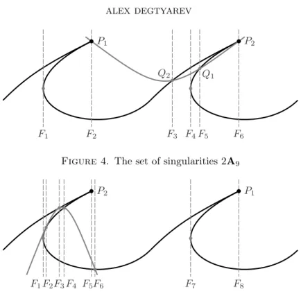
3.3. The set of singularities 2A9. The sextic B is the double covering of ¯B
ramified at a section ¯L passing through both cusps of ¯B, see Figure 4; one can take
for ¯L the transform of the secant ¯L1shown in Figure 2.
We choose the generators α, δ, β, γ in a nonsingular fiber between F4 and F5.
Then, there are relations [γ, β] = 1, β = γ, and [δ, α] = 1 (from F5, F4, and F3,
respectively); due to Lemma 3.2.6, the group is D10× Z3.
3.4. The set of singularities 4A4⊕ 2A1. The curve B is the double covering
of ¯B ramified at a section ¯L double tangent to ¯B, see Figure 5. (The existence of a
F6 F5 Q1 F4 F3 Q2 F2 F1 P1 P2
Figure 4. The set of singularities 2A9
F8 F7 F6 F5 F4 F3 F2 F1 P2 P1
Figure 5. The set of singularities 4A4⊕ 2A1
is rather obvious geometrically: one moves a sufficiently sharp parabola to achieve two tangency points. An explicit construction of a pair ( ¯B, ¯L) using equations is
found in Section 4.6 and Figure 8 below.)
We choose the generators α, β, δ, γ in a nonsingular fiber between F4 and F5.
Ignoring the cusp F8, see Lemma 3.2.4, the relations for Π are
(3.4.1) (αβ)2α = β(αβ)2 (from the cusp F 5),
(3.4.2) [β, δ] = [γ, δ] = 1 (from F4 and F6),
(3.4.3) (αδ)2= (δα)2 (from F3),
(3.4.4) (α−1δαβ)2= (βα−1δα)2 (from F 2),
(3.4.5) γ = (α−1δα)−1β(α−1δα) (from the tangent F1),
(3.4.6) γ−1αβα−1γ = (αβ)α(αβ)−1 (from the tangent F
7),
(3.4.7) (αβδγ)2= 1 (patching F∞).
(The relations are simplified using (3.4.2).) The corresponding group π given by Proposition 3.2.5 was analyzed using the GAP software package. According to GAP,
π is an iterated semi-direct product Z3× ((((Z2× Q8) o Z2) o Z5) o Z2), and the
abelian factors of its derived series are as stated in Theorem 1.2.1. (Here, Q8is the
order 8 subgroup {±1, ±i, ±j, ±k} ⊂ H.)
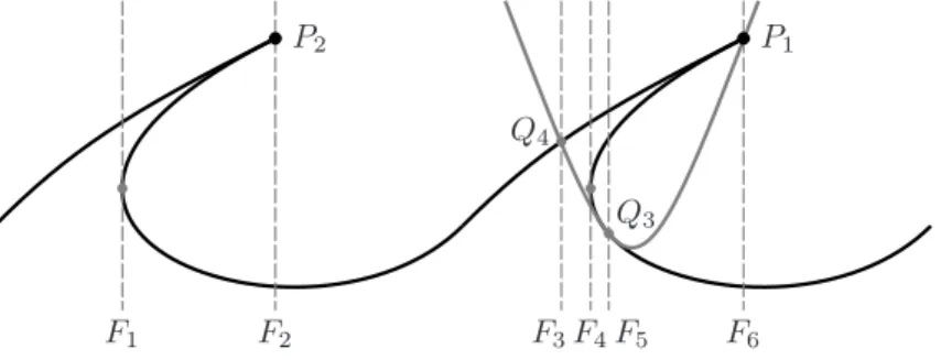
3.5. The set of singularities A9⊕2A4⊕A2. The curve B is the double covering
of ¯B ramified at a section ¯L inflection tangent to ¯B, see Figure 6. One can take
for ¯L the transform of the tangent ¯L2 shown in Figure 2; an explicit construction
F6 F5 Q3 F4 F3 Q4 F2 F1 P2 P1
Figure 6. The set of singularities A9⊕ 2A4⊕ A2
We choose the generators α, β, γ, δ in a nonsingular fiber between F4 and F5.
Ignoring the vertical tangent F1, see Lemma 3.2.4, the relations for Π are
(3.5.1) β = γ (from the tangent F4),
(3.5.2) [α, γδγ−1] = 1 (from F
3),
(3.5.3) (γδ)3= (δγ)3 (from F5),
(3.5.4) [αβ, δ1] = 1 (from the cusp F6),
(3.5.5) δ1(αβ)2α = β(αβ)2δ1 (from the cusp F6),
(3.5.6) (β2γ)2β2= γ(β2γ)2 (from the cusp F2),
(3.5.7) (αβγδ)2= 1 (patching F∞),
where δ1 = (γδγ)δ(γδγ)−1 and β2 = (αγδ−1γ−1)β(αγδ−1γ−1)−1. The resulting
group π, see Proposition 3.2.5, was analyzed using GAP. Its derived series is as stated in Theorem 1.2.1.
3.6. The sets of singularities A9⊕ 2A4⊕ A1 and 4A4⊕ A2. For the set of
singularities A9⊕2A4⊕A1, we perturb the inflection tangency point Q3in Figure 6
to a simple tangency point and a point of transversal intersection. Then, (3.5.3) is replaced with [γ, δ] = 1 and one obtains [α, δ] = 1 (from (3.5.2) ), δ1 = δ, and
[β, δ] = 1 (from (3.5.4) ); due to Lemma 3.2.6, the resulting group π is D10× Z3.
For the set of singularities 4A4⊕ A2, the intersection point P1 in Figure 6 is
perturbed to two points of transversal intersection. Then, (3.5.4) and (3.5.5) turn into [α, δ1] = [β, δ1] = 1 and (αβ)2α = β(αβ)2, respectively. Using GAP shows that
the resulting group π is D10× Z3.
3.7. The sets of singularities A9⊕ 2A4 and 4A4⊕ A1. These sextics can be
obtained by small perturbations from sextics with the sets of singularities, e.g., 2A9 (see 3.3) and A9⊕ 2A4⊕ A1(see 3.6), respectively; the resulting groups have
already been shown to be isomorphic to D10× Z3.
4. The equations
The calculations in this section (substitution, factorization, discriminants, and system solving) are straightforward but rather tedious. Most calculations were performed using Maple.
4.1. The curve ¯B. In appropriate affine coordinates (x, y) in Σ2 the trigonal
curve ¯B with two type A4 singular points is given by the Weierstraß equation f (x, y) = 4y3− 3yp(x) + q(x) = 0, where
(4.1.1)
p(x) = x4− 12x3+ 14x2+ 12x + 1, q(x) = (x2+ 1)(x4− 18x3+ 74x2+ 18x + 1).
The discriminant of (4.1.1) with respect to y is ∆ = (2)10(3)6x5(x2− 11x − 1); it
has two 5-fold roots x = 0 and x = ∞ (the singular points of ¯B) and two simple
roots x± = 11/2 ± 5√5/2 (the two vertical tangents).
Remark. The point x = ∞ is a 5-fold root of ∆ as the ‘predicted’ degree of ∆ is 12.
Originally, equation (4.1.1) was obtained by an appropriate birational coordinate change from the equation y2 − 2x2y + x4− 4x3y of the quartic with the set of
singularities A4⊕ A2, see Figure 2.
The curve ¯B is rational; it can be parametrized as follows
(4.1.2) x(t) = t 2(t − 1)
t + 1 , y(t) =
(t2+ 1)(t4− 2t3− 6t2+ 2t + 1)
2(t + 1)2 .
The special points on the curve correspond to the following values of the parameter:
(4.1.3)
t0= 0, t∞= ∞ (the cusps),
t0
0= 1, t0∞= −1 (the points under the cusps),
t±= −1 2∓
1 2
√
5 (the tangency points over x = x±),
t0 ±= 2 ±
√
5 (the other points over x = x±).
Both the curve and the parametrization are real, as are all singular fibers of ¯B.
Furthermore, ¯B is invariant under the automorphism x 7→ −1/x, y 7→ y/x2. In the t-line, this transformation corresponds to the automorphism t 7→ −1/t.
4.2. Generic sextics. Due to Theorem 2.1.1, any D10-sextic is given by an affine
equation of the form
(4.2.1) f (x, y2+ x2+ bx + c) = 0,
where f (x, y) is the polynomial given by 4.1.1 and y = ax2+ bx + c is the equation
of the section ¯L constituting the branch locus. Conversely, from Theorem 3.2.8
it follows that any curve B given by (4.2.1) is a D10-sextic provided that it is
irreducible and all its singularities are simple. Note that B is reducible (splits into two cubics interchanged by the involution on P2) if and only if, at each point of
intersection of ¯B and ¯L, the local intersection index is even. Hence, in view of
the classification of sections given below, B is reducible if and only if it has the (non-simple) set of singularities Y1
1,1 ⊕ A9, see 4.3; such a curve splits into two
cubics with a common cusp.
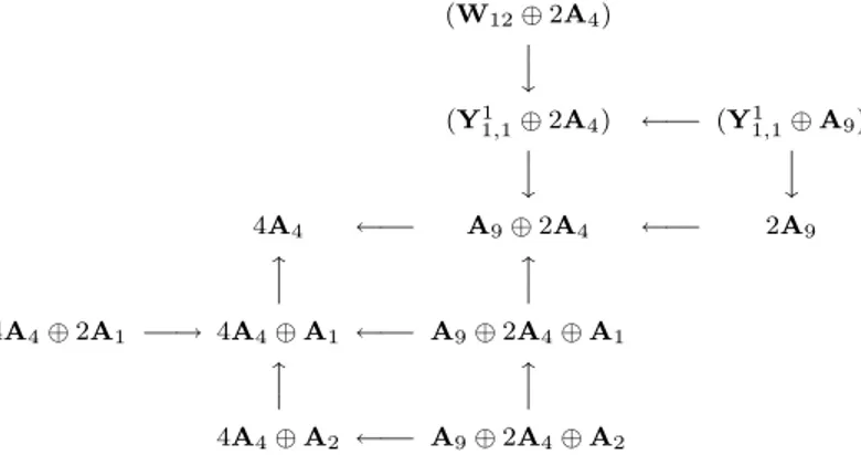
The set of singularities of a sextic B given by (4.2.1) with a generic triple (a, b, c) (so that ¯L is transversal to ¯B) is 4A4. In Sections 4.3–4.7 below, we discuss the
(Sometimes, the condition is stated using an extra parameter t, as an attempt to eliminate t results in a multi-line Maple output.) For each degeneration, we use Lemmas 2.3.2 and 2.3.3 to indicate the set of singularities of the corresponding sextic B. The results should be understood as follows: a sextic B given by (4.2.1) has a certain set of singularities Σ if and only if the triple (a, b, c) satisfies the con-dition corresponding to Σ but does not satisfy any concon-dition corresponding to an immediate degeneration of Σ (see the adjacency diagram shown in Figure 7).
(W12⊕ 2A4) ? ? y (Y1 1,1⊕ 2A4) ←−− (Y1,11 ⊕ A9) ? ? y ? ? y 4A4 ←−− A9⊕ 2A4 ←−− 2A9 x ? ? x ? ? 4A4⊕ 2A1 −−→ 4A4⊕ A1 ←−− A9⊕ 2A4⊕ A1 x ? ? x ? ? 4A4⊕ A2 ←−− A9⊕ 2A4⊕ A2
Figure 7. Immediate adjacencies of sets of singularities
For completeness, we also mention (parenthetically in Figure 7) the sextics B given by (4.2.1) whose singularities are not simple; this is the case if and only if the triple (a, b, c) is as in (4.3.2) below. In Arnol0d’s notation, B may only have a non-simple singular point of one of the following two types: Y1
1,1(transversal intersection
of two cusps) or W12 (semiquasihomogeneous singularity of type (4, 5) ).
4.3. Sections through singular points. A section y = ax2+ bx + c passes
through one of the cusps of ¯B (the set of singularities A9⊕ 2A4) if and only if
(4.3.1) c = 1
2 (the cusp at t = 0) or a = 1
2 (the cusp at t = ∞). Hence, the section passes through both cusps (the set of singularities 2A9) if and
only if a = c = 1/2.
Further degenerations considered here produce sextics with a non-simple singular point. The section is tangent to ¯B at a cusp (the set of singularities Y1
1,1⊕ 2A4) if and only if (4.3.2) c = 1 2, b = 3 (at t = 0) or a = 1 2, b = −3 (at t = ∞). It passes through the other cusp (the set of singularities Y1
1,1 ⊕ A9; this sextic
is reducible) if and only if a = c = 1/2 and b = ±3. Finally, the section passes through a cusp with local intersection index 5 (the set of singularities W12⊕ 2A4)
if and only if (4.3.3) (a, b, c) = ³ −11 2 , 3, 1 2 ´ or (a, b, c) =³ 1 2, −3, − 11 2 ´ .
Such a section cannot pass through the other cusp.
A section passing through both cusps of ¯B or tangent to ¯B at a cusp does
not admit any degenerations other than described above. Indeed, if a = c = 1/2 (respectively, c = 1/2 and b = 3), then, restricting the original polynomial f (x, y) to the section and reducing the trivial factor x2 (respectively, x4), one obtains a
polynomial in x whose discriminant is 16(b − 3)3(b + 3)3(respectively, 12(2a − 1)5). Remark. According to [3], D10-sextics are characterized by the existence of two
conics in a very special position with respect to the type A4and A9singular points
of the curve. These conics are the pull-backs of the two sections y = ax2+ bx + c
with a = c = 1/2 and b = ±3, each section being tangent to ¯B at one of its cusps
and passing through the other cusp.
4.4. Digression: other generalized D10-sextics. From 4.3, it follows that the
double covering construction also produces representatives of the two families of irreducible generalized D10-sextics with a quadruple singular point, see [3]. (In each
family, symmetric curves form a codimension one subset.) It is worth mentioning that the remaining classes of irreducible generalized D10-sextics, those with the sets
of singularities J2,0⊕ 2A4, J2,1⊕ 2A4, and J2,5⊕ A4, see [4], are also related to the
trigonal curve ¯B ⊂ Σ2with two type A4singular points: they are obtained from ¯B
by a birational transformation rather than double covering. 4.5. Simple and double tangents. Let
(4.5.1) s(t) = ax2(t) + bx(t) + c,
where x(t) is given by (4.1.3). Solving s(t) = y(t) and s0(t) = y0(t), one concludes that a section y = ax2+ bx + c is tangent to ¯B at a point (x(t), y(t)) ∈ ¯B (the set
of singularities 4A4⊕ A1) if and only if
(4.5.2) a =−b(t 3+ 2t2− 1) + t5− 5t3− 5t2− 3 2t2(t − 1)(t2+ t − 1) , c = −bt2(t3− 2t + 1) + 3t5+ 5t3− 5t2+ 1 2(t + 1)(t2+ t − 1)
for some b ∈ C and t ∈ C r {0, ±1, t±} or
(4.5.3) t = 1 and (b, c) = (−6, −1) or t = −1 and (a, b) = (−1, 6).
This section passes through the cusp of ¯B at t = 0 (the set of singularities A9⊕
2A4⊕ A1) if and only if c = 1/2, see 4.3; in this case
(4.5.4) a = t 4− t3− 2t2+ 3t + 11 2(t − 1)2(t2+ t − 1) , b = − 3(t3+ 2t − 1) (t − 1)(t2+ t − 1), c = 1 2. The section passes through the cusp of ¯B at t = ∞ (another implementation of the
set of singularities A9⊕ 2A4⊕ A1) if and only if a = 1/2, see 4.3; in this case
(4.5.5) a = 1 2, b = − 3(t3+ 2t2+ 1) (t + 1)(t2+ t − 1), c = − 11t4− 3t3− 2t2+ t + 1 2(t + 1)2(t2+ t − 1) .
Relations (4.5.4) and (4.5.5) still hold for the exceptional values t = −1 and t = 1, respectively, cf. (4.5.3).
There is a somewhat unexpectedly simple relation between the two tangency points of a section double tangent to ¯B. We state it below as a separate lemma.
Denote by ²±the roots of the polynomial t2+ 3t + 1. One has ²±= (−3 ±√5)/2 = t±/t0±. Note that ²+²−= 1.
4.5.6. Lemma. Let ¯B ⊂ Σ2 be the trigonal curve parametrized by (4.1.2), and let t1, t2 ∈ C r {0, t±} be two distinct values of the parameter. Then, there is a
section tangent to ¯B at both points (x(ti), y(ti)), i = 1, 2, if and only if t2/t1= ²±. Proof. Assume that t1, t26= ±1. (The case when one of t1, t2takes an exceptional
value ±1 is treated similarly using (4.5.3).) Let a1, a2and c1, c2be the coefficients a
and c in (4.5.2) evaluated at t = t1, t2, respectively. Then a1− a2= c1− c2 = 0;
hence, (a1− a2)t21t22(t1− 1)(t2− 1) + (c1− c2)(t1+ 1)(t2+ 1) = 0. The latter
expression takes the form
3(t1− t2)3(t12+ 3t1t2+ t22)
(t2
1+ t1− 1)(t22+ t2− 1) = 0,
and, taking into account the restrictions on t1, t2, one obtains t2/t1 = ²±. For
the converse statement, one observes that, if t2/t1 = ²±, then the linear system a1= a2, c1= c2 in one variable b has a solution (given by (4.5.7) below). ¤
Thus, a section y = ax2+ bx + c is double tangent to ¯B (the set of singularities
4A4⊕ 2A1) if and only if (4.5.7) b = b± = −3(t 2+ (3²∓+ 1)t − ²∓)(t2− ² ±t − ²∓)(t + t±) (t − t±)(t − t∓)2(t − t0 ±)2 .
Here, the two tangency points are at t and ²±t; the expressions for a and c are
obtained by a direct substitution to (4.5.2). This relation still holds if t = ±1. A section tangent to ¯B at a smooth point does not admit any other degenerations.
Indeed, sections passing through both singular points of ¯B or tangent to ¯B at a
singular point are considered in 4.3, and sections inflection tangent to ¯B are treated
in 4.7 below. A section cannot be tangent to ¯B at three smooth points at t = t1, t2,
and t3, as then one would have t2/t1= ²±, t3/t2= ²±, and t3/t1= ²±; this system
is incompatible unless t1 = t2 = t3 = 0. Finally, a double tangent cannot pass
through a singular point, say at t = 0, as substituting t = t1 and t = t2 to (4.5.4)
and eliminating a and b, one obtains a system in (t1, t2) which has no solutions
with t16= t2.
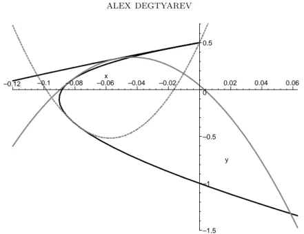
4.6. Digression: the curve in Figure 5. The pair ( ¯B, ¯L) used to calculate the
fundamental group of a sextic B with the set of singularities 2A4⊕ 2A1, see 3.4
and Figure 5, can be obtained from (4.5.7) and (4.5.2) with the following values of the parameters: t1= t = 1/2 and t2= ²+t1≈ −0.191. Then one has a ≈ −161.05, b ≈ −13.93, and c ≈ 0.0448. The two points of transversal intersection of ¯B and
the section y = ax2+ bx + c are at t ≈ 0.281 (over x ≈ −0.0442) and t ≈ 1.101
(over x ≈ 0.0585). This section is shown in Figure 8.
4.7. Inflection tangents. A section y = ax2+ bx + c is inflection tangent to ¯B
at a point (x(t), y(t)) ∈ ¯B (the set of singularities 4A4⊕ A2) if and only if
(4.7.1) a =t 6+ 3t5− 5t3+ 12t + 11 2(t2+ t − 1)3 , b = −3(t 2+ 1)(t4+ 3t3− t2− 3t + 1) (t2+ t − 1)3 , c = −11t 6− 12t5+ 5t3− 3t + 1 2(t2+ t − 1)3 ,
–1.5 –1 –0.5 0 0.5 y –0.12 –0.1 –0.08 –0.06 –0.04 –0.02 0.02 0.04 0.06 x
Figure 8. Maple plot of the curve ¯B (black), a double tangent (solid
grey), and an inflection tangent through a singular point (dotted grey)
t ∈ C r {0, t±}. (To see this, one should solve for (a, b, c) the system s(t) = y(t),
s0(t) = y0(t), s00(t) = y00(t), where s(t) is the section given by (4.5.1).) This inflection tangent passes through one of the cusps of ¯B (the set of singularities
A9⊕ 2A4⊕ A2) if and only if t = 3/4 (the cusp at t = 0) or t = −4/3 (the cusp at t = ∞). The corresponding values of (a, b, c) are
(4.7.2) (a, b, c) =³ 3077 10 , 177 5 , 1 2 ´ and (a, b, c) =³ 1 2, − 177 5 , 3077 10 ´ ,
respectively. The section corresponding to t = 3/4 is shown in Figure 8.
An inflection tangent at a smooth point of ¯B cannot have any other
degen-erations. Indeed, after clearing the denominators and reducing the trivial factor (u − t)3, the equation y(u) = ax(u)2+ bx(u) + c with a, b, and c given by (4.7.1)
and x( · ), y( · ) as in (4.1.2) has solution u = t only for t = 0 or t± (hence, no quadruple intersection points), and the discriminant of the above equation with respect to u is, up to a constant coefficient, t2(3t + 4)(4t − 3)(t2+ t − 1)3 (hence,
no other tangency points).
References
1. A. Beauville, Application aux espaces de modules, G´eom´etrie des surfaces K3: modules et p´eriodes, Ast´erisque, vol. 126, 1985, pp. 141–152.
2. A. Degtyarev, On deformations of singular plane sextics, J. Algebraic Geom. 17 (2008), 101–135.
3. A. Degtyarev, Oka’s conjecture on irreducible plane sextics, arXiv:math.AG/0701671. 4. A. Degtyarev, Oka’s conjecture on irreducible plane sextics. II, arXiv:math.AG/0702546. 5. A. Degtyarev, Zariski k-plets via dessins d’enfants, arXiv:math/0710.0279.
6. A. Degtyarev, M. Oka, A plane sextic with finite fundamental group, this volume.
7. C. Eyral, M. Oka, On the fundamental groups of the complements of plane singular sextics, J. Math. Soc. Japan 57 (2005), no. 1, 37–54.
8. C. Eyral, M. Oka, On a conjecture of Degtyarev on non-torus plane curves, this volume. 9. Derek F. Holt, W. Plesken, Perfect Groups. With an appendix by W. Hanrath, Oxford Math.
Monographs, Oxford University Press, New York, 1989.
10. E. R. van Kampen, On the fundamental group of an algebraic curve, Amer. J. Math. 55 (1933), 255–260.
11. V. V. Nikulin, Integer quadratic forms and some of their geometrical applications, Izv. Akad. Nauk SSSR, Ser. Mat 43 (1979), 111–177 (Russian); English transl. in Math. USSR–Izv. 43 (1980), 103–167.
12. O. Zariski, On the problem of existence of algebraic functions of two variables possessing a
given branch curve, Amer. J. Math. 51 (1929), 305–328.
Department of Mathematics, Bilkent University, 06800 Ankara, Turkey