Move based heuristics for the unidirectional loop network layout problem

(1)

E-Z9OOO(LS)LlZZ-LLEOS IId ‘ Pam== VI% IIV 'A'8 ="??z J?~~wl8661 0 00'61$/86/LIZZ-LLEO S~U~SXII 30 aDuanbas aqj saypads lt~ql wd qDea 103 uay% s! ueld ssaDold v TIO~QS (mu) p~~olun/peo~

aql

1~ Urals,& aql sl!xa pm! ualua tred ~SKJ *(s~gv) salD!qaA pap@ paleruolne leuogDa.up!un 30 sqled ary 10 ‘suralsrCs I~SX~UOLII ptzaqJaA0 ‘sauq ~01 ‘ s.IodaA -UOD dool Lq paAlas ual3o ala slnodq 30 sad& asau *asfMyo13 *%*a ‘ uoyal!p auo Quo u! pauodsueq an?

slapapqq

‘ awo 6113tzxa uoyl~s qaea @no’ql %u!ssvd qled Ou!Ipuaq lt+alm e 6q palDauuo3 aE suo!l~s 8u!u!qDwu 11~ *dool e u! pa%elra are sau!q3wu ‘ lnohl (em) yJomlau dool p?uoy9aqp!un e UI *(26fjl ‘ my pue sgahnox ~0 scyls!maq uo!lDnrlsuoD aql se IlaM se) poqlaw a%eq3~alu! as+ -qtzd aql ueql urnuydo arw aql u1o.13 suo!le!Aap uuuu! -xw_u pun a8waAe 30 seal u! Jallaq dlwlo3!un twopad asodoJd aM sys!lnaq aql leql alwpu! sllnsal lsal Jno .@suap MOW 30 slaaal luaJaJJ!p putz sau!q3euI 0s 01 s :IpuI-a ‘9ZIp 99~ ZIE 06-k :XZd IOWV3 %I~pUOdSaUO~. tuol3 az!s u! %u@n2J sa3uelsu! uropue~ egg uo pasvq a.InltXal!~ aql u10.13 s3!lspnaq %ys!xa Jay10 ql!M pand -INOD s! scyspnaq asay ssaua+vaga Iwopwndtuo:, au . (lanbas aql u! pauyap aq 01) ,saAotu lauol!sod, uo paseq an? q3!qM s3!lsyaq 0~1 asodold put? I.uaI -qord aql30 uoyk?~nuuoJ1no ah!% aM'sau!qxtu uaaM1 -aq saXIEls!p sauy smog ued 30 uIns aql Aq pauyap is03 uuxu!u!tu aqi%u!p~a!Lsauyqxr 3oluaunB~sse ue au!uxlalap 01 s! aApDa[qo au *luauIuo+ua SW uv u! yowlau do01 Ieuoya.np!un e u! sau!qwu %U@IOJ.IR Llleuydo 30 uralqold aql .~ap!suo~ aM ladEd s!ql UI

uoympoqq

??

I

Ja!r\as[g 8661 @ 3psyaq a&n?q31alu! as!ml!ad UMOU~ Ilam aql 01 uos$duroD u! axmuo$md Jouadns L~oJyIn saW!pu! SxlsyIaq paSeq ahour-OMJ ql!~ UO!)ElUaUIpadXa leuogwndruo~ mo ‘ alnlelalg 8ugSfXa aql u! U8FSap 3p.Uqlf.1O%lE OJU! hM a! pun03 lou saq Sah0u.I JO idamos aql q%noql uahg ~sa%ueq3~alu~ (hem-z dl.ruIm!ued) km-y JO SaAouI uo paseq suIqlyo8Ie PauIaAoJdm! @301 pua saAoouI leuo!l!sod JO cap! aq] ssnmp a& malqold pnq lClah e dlleuogelndmo:, s! qxqm uraIqoId luauu@ss~ xlelpenb e u! slInsaJ waIqoJd aql JO uo!lepwuoJ aqJ, .amrrls!p MOB 1~101 aql azwgu 01 dool e puno.m suogmo[ alqEl!em u u! paxId aq lsnw sau!qmu u aJaqM uralsk %uywe~nuew e u! tuaIqoJd 1noLeI ylomlau dooI aql lap!suoD a& 8P-9E (8661) 801 VJ=Wl @"WJJ~O KJ @"JW ~'JJ"EI HOUV3S38

lVNOllVMdO

JO

lVNkinOr

NEldOkln3

(2)

B.C. Tansel, C. BikdEuropean Journal of Operational Research IO8 (1998) 3648 31

the part must visit to complete its processing. When a part’s operation is completed on a machine, it is moved to its next machine on the unicyclic material handling network. If the workstation is occupied, the part is stored in a local buffer, waiting for the workstation to become free.

ULN layouts are preferred to other configurations due to their relatively lower initial investment costs because they contain a minimal number of required material links to connect all workstations while providing a high degree of material handling flexibility (Afentakis, 1989). Such configurations are able to satisfy all material handling requirements for the part types scheduled for manufacturing in the system as there is at least one directed path connecting any pair of workstations. With these layouts, future introduc- tion of new part types and process changes are easily accommodated. Of the 53 FMSs in Japan, surveyed by Jaikumar and Van Wassenhove ( 1989), ULN layouts are the most common architecture. These systems also have lower operational complexity. Gaskins and Tanchoco (1987) point out that bidirectional material handling paths require more sophisticated control and higher installation costs than unidirectional paths. This makes bidirectional paths a less favored altema- tive than unidirectional loop networks.

The Unidirectional Loop Network Layout Problem (ULNLP) is generally formulated as a Quadratic As- signment Problem (QAP). The objective is to assign each machine to exactly one of the candidate locations such that an appropriate objective function is mini- mized. Two types of objective criteria have been used in the literature:

( I ) minimization of the sum of flows times distances per unit time (Bozer and Rim, 1989, Kiran and Karabati, 1988, and Kiran, Unal and Karabati, 1992).

(2) minimization of the total number of parts that cross the LUL station per unit time (Afentakis,

1989, and Kouvelis and Kim, 1992).

It can be shown that the two objective criteria are equivalent (Kouvelis and Kim, 1992; Tansel and Bilen, 1994).

Various versions of the problem have received attention in the literature. Bozer and Rim ( 1989) present a linear programming (LP) relaxation for ULNLP with equal spaced locations and claim that the LP solves

the equal spaced ULNLP optimally. However, we have not been able to validate their proof. If their result is true, then this identifies the equal spaced ULNLP as a polynomial time solvable case of the QAP If true, this would be an important polyhedral result because the non-equal spaced ULNLP is known to be NP-hard (Kouvelis and Kim, 1992). We remark that the non- equal spaced ULNLP with Q conserved (balanced) Jlow matrix (i.e. for each station, the total material

flow into a station is the same as the total outflow from that station) is equivalent to the equal spaced ULNLP (Bozer and Rim, 1989; Kiran, Unal and Kara- bati, 1992). Hence, the conserved flow version of the non-equal spaced ULNLP is also polynomially solvable if Bozer and Rim’s result is true. Kiran, Unal and Karabati ( 1992) report that integer solutions are obtained from the LP relaxation of their formulation of the conserved flow problem. However, their test runs are restricted to problems with up to six stations. For larger problems we discovered in our test runs that noninteger solutions are possible. This of course raises questions on the validity of Bozer and Rim’s ( 1989) result in the optimality of the LP relaxation for the equal spaced problem.

For the non-conserved flow, non-equal spaced ULNLP, the problem is formulated as a QAP with a special cost matrix (due to the circularity of the loop which induces a special distance matrix). Kouvelis and Kim ( 1992) proved that the problem is NP-hard by transforming it to the feedback arc set problem which was suggested earlier by Afentakis ( 1989).

Bozer and Rim (1989) developed a lower bound by modifying the well known Gilmore-Lawler bound. They took advantage of the circularity of the distance matrix. Kiran and Karabati ( 1988) introduced an exact solution algorithm with a branch and bound (B&B) structure similar to that of Gilmore ( 1963) and Lawler ( 1963). Computations of the lower and upper bounds are presented. If there is a large number of buffer spaces interacting independently with the loop network, then these buffer spaces should be treated as separate stations. In such cases, the number of stations increases and the B&B algorithm will not be efficient. Kiran and Karabati ( 1988) developed a polynomial approximation algorithm based on filtered beam search technique. Kouvelis and Kim (1992) gave three heuristic procedures, KK- 1, KK-2, and KK-

(3)

38 B.C. Tansel. C. Bilen/European Journal of Operational Research 108 (1998) 36-48

3,

that are supported by some dominance rules. The

dominance rules suggest locating a machine to the last

position if it has only incoming flows from other ma-

chines. Similarly, a machine that has only outgoing

part flows should be assigned to the first position. Also

they developed an optimal B&B algorithm.

Some special cases have also been noted in the lit-

erature, Bozer and Rim ( 1989) proved that if the flow

matrix is symmetric, that is to say

Wij = Wji

for all i, j,

interchanging machines

i

and j does not change the

objective function value. Hence, any layout is optimal

when the flow matrix is symmetric. Kiran and Karabati

( 1988) give a polynomially solvable (O( n* log(n) )

special case of the problem when parts are transported

to a LUL station after every operation.

Leung ( 1992) considers the ULNLP problem

with the objective of minimizing the maximum num-

ber of times a part family traverses the loop before

its processing is completed. They call this prob-

lem the min-max reload loop-layout problem. Based

on graph-theoretic arguments, a heuristic is devel-

oped which constructs a layout from a solution to

the linear-programming relaxation of the problem.

Millen, Solomon and Afentakis ( 1992) consider the

impact of the number of LUL stations in automated

manufacturing systems with unidirectional closed

loop material handling equipment. Comparison of

material handling costs for two cases (single LUL

station and a LUL station for each machine) indicated

that providing flexibility in part entry/exit functions

reduces material handling movement.

The rest of our paper is organized as follows: in

Section 2, we give our formulation of the problem,

which is a special case of the well known quadratic

assignment problem. In Section 3, we introduce and

discuss the idea of positional moves. In Section 4,

we present two improvement type heuristic methods

based on positional moves. In Section 5, we discuss the

computational effectiveness of the proposed heuristics.

Section 6 ends the paper with concluding remarks.

2.

Unidirectional loop network layout problem

formulation

The unidirectional loop network layout problem

(ULNL) can be stated as follows:

Given machines

0, 1, . . . , n,

with machine 0 being

the Load/Unload (LUL) station, candidate positions

labeled

0, 1, . . . , n

and pairwise non-symmetric part

flows between machines, what is the assignment of

the machines to candidate positions that yields the

minimum cost defined by the sum of partflows times

distances between the machines?

We assume the LUL station is preassigned to lo-

cation (position) 0. The remaining machines are to

be assigned to candidate locations 1,

. . . , n

around the

loop. The material movement is unicyclic, and it is

assumed to be in the clockwise direction.

First we discuss how the part flows are determined

from process plans. In an FMS environment, machines

are capable of processing different part types simulta-

neously.LetP={l,...

, p}

be the set of different part

types to be processed in the system per period. Each

part type may require different routes for their pro-

cessing. By a route, we mean the sequence in which a

part visits the machines in the system. This sequence

is given by a process plan, Zp, for a particular part type

p E

P. For example, if part type 2 needs to be pro-

cessed by three machines in the order, machine 3, ma-

chinel,andmachine2,thenZz=(3,1,2).Letn~be

the number of times machines

i

and j appear consec-

utively (in that order) in the process plan Z,. Equiv-

alently, nc specifies the number of moves to be made

from machine

i

to machine j by part type

p.

Let up be

the number of units of part type

p

to be produced per

time period.

With these definitions, the

part$ow

from machine

i

to machine j per time period is the quantity

Wij =

c

v&

for all

i, j,

with

i # j.

PEP

Observe that Wij # Wjj in general.

Let N = {l,...,

n} be the station (machine) in-

dices and put fl=

NU{O}.

We take Wjj = 0,

Vi E i@,

while wij is the quantity defined above for

i, j E fl,

with

i # j.

For a given machine

i,

the total inflow and outflow

associated with machine

i are the

quantities

R(i) = Cwji

and C(i) = CWij.

(4)

B.C. Tansel, C. Bilen/European Journal of Operational Research 108 (1998) 36-48

Fig. I. Loop network locations. Fig. 2. Determination of the distance from location 1 to k

We say the system is balanced if R(i) = C(i) for all

i E I@‘. We call the flow matrix W = [ wij] a conserved flow matrix if the system is balanced.

Generally, an automated manufacturing system is balanced when no manual interruption is permitted so that any part entering the system will surely exit the system. The balancedness assumption need not hold in systems with multiple LUL stations (note that the manual removal of a broken part may be viewed as an unload operation at that machine).

(4) & + dk, 2 &,,

QL km.

Due to the assumption of unit spacing between adjacent locations, the distance from location 1 to k is determined by (see Fig. 2)

k-l if k > 1,

dlk =

{

n+l-l+k ifk<l, 0 if k = 1.

Define a machine assignment vector to be a permu- tation of the integers 1,2,. . . , n, and denote it by Assumptions underlying the formulation are as fol-

lows: a= (a(l),...,a(n)), Al. A2. A3. A4. A.5.

The location of the LUL station is fixed at position 0.

The system is balanced.

Adjacent locations are unit distance apart (since the system is balanced, the distance between machines is of no importance, as proved in Bozer and Rim, 1989, and Kiran, Unal and Karabati, 1992).

Process plans and the number of units to be produced for each part type are given, so that pairwise part flows between machine pairs can be calculated.

Parts enter and exit the system at the LUL station.

Let the locations around the loop network be num- bered O,l,..., n in increasing order of indices in clockwise direction (see Fig. 1). Assumption A3 implies the distance between any two adjacent locations is one and the total length of the loop is n + 1. Let dlk be the transport distance from location 1 to location k. This distance has the following properties:

(l) d’k _{L 0 for 1 # k

-0 iffl=k, (2) d,k # dk, in general. ’

(3) dlk-l-dk[=n+l,Vl,kE{O ,..., n},l # k.

where cu( i) specifies the location of machine i. Let II be the set of all permutations of 1,2, . . . , n.

The total material handling distance per period for a given assignment (Y is

+il

woidoaci)

-I-

c

n

Wida(i)O~

i=l i=l

The first summation in the definition of Z ( (Y) accounts for the material flow between machines, the second (third) summation accounts for the material flow from (to) LUL station to (from) all machines.

Observe that doa is simply a(i), and da(i)0 is n + 1 - a(i) .

Hence, an equivalent definition of Z ( CX) is

Z(a) =

C C

wijdrr(i)a(j)

+

C(woi -

wio)a(i)

i=l j=l i=l

+cn +

l)R(O).

Note that the last term is a constant and does not affect the minimization.

(5)

40 B.C. Tansel. C. BilenIEuropean Journal of Operational Research 108 (1998) 36-48

Then the ULNL problem can be stated as that of

finding an assignment vector LY that minimizes the

expression 2 (a)

:

(ULNLP)

ran; Z(cu).

This formulation is a special case of the QAP The

special structure results from the stated properties of

the distance matrix and the balancedness assumption.

It is well known that QAP is NP-hard with reported

computational success limited to less than 18 ma-

chines (Burkard, 1990; Burkard and Stratman, 1978).

Whether or not the special distance matrix may lead

to efficient exact methods is an open question.

3. Local

optimality, interchanges, positional moves

A commonly used criterion to solve QAP is the

steepest descent criterion of pairwise interchanges. For

example, the well known CRAFT algorithm (Francis,

McGinnis and White, 1992) relies on pairwise inter-

changes between departments to reduce the score of a

layout which is computed by the sum of flows times

distances. The idea is to begin with a seed layout and

perform pairwise interchanges as long as the objec-

tive value is reduced by a positive amount. Termina-

tion occurs when no pair interchange gives any im-

provement. Such a solution is a locally optimal one.

It may be possible to improve it if one takes k-way

interchanges into account where

k 2

3. Given two assignment vectors (Y and 6, we define

(Y and ti to be k-way neighbors if there exist

k

distinct

position indices

41, . . . , qk

such that

a(qi) #&(qi)

for

i =

1,.

. . , k,

while

a(j)=c(j)

for j

$!{q19...,qk}.

The

definition implies (Y and 6 are identical in n -

k

position while they are non-identical in each of the

remaining

k

positions. Let Nk( cu) be the set of all

k-

way neighbors of cy and define

CNk(&‘) =U{Nj(o)

:

1 < j 6

k}.

We say an assignment vector (Y is a

k-way local opti-

mum

if

z(a)

6 z(6’)

Qc E CNI,(cu).

Observe that

k = n

implies global optimality.

Let us call a heuristic method a

k-way heuristic

(or

a k-way interchange method) if it seeks a k-way lo-

cal optimum by performing

k

or fewer interchanges.

Even though one may be tempted to think that a k-way

heuristic should always find a locally optimal assign-

ment that is at least as good as one found by a h-way

heuristic where 2 <

k,

this is not true in general. For

example, a 2-way heuristic may find a better solution

than a 3-way or a 4-way heuristic for a given problem

instance. Despite that, it is generally expected that,

for

k < &,

a i&way heuristic may perform better on

the average than a k-way heuristic, since k-way inter-

changes take into account k-way interchanges.

There is also the computational burden one must

take into account. For example, a 2-way heuristic re-

quires U( n*) comparisons per iteration while a k-way

interchange method searches over O( x:Z2 j! (II>

)

neighbors. The additional computational burden is

usually not justified on the basis of possible additional

improvements over 2-way interchanges.

We now focus on a new ‘neighbor’ concept which

has not been utilized in the literature. It is based on

‘positional moves’ and leads to an 0(n*) local im-

provement method whose average performance is bet-

ter than the pairwise interchange method which is also

O(n*).

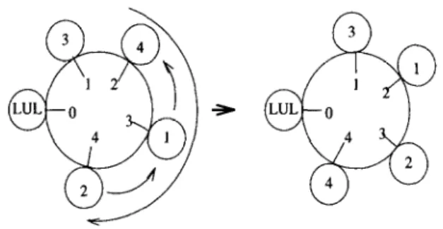
Given an assignment vector, a positional move is

made by moving a machine from its current position

to one of the other candidate positions, and shifting

all affected machines by one position down in counter

clockwise direction. The affected machines are those

that occupy the positions in the

clockwise

direction

between the old and new positions of the moved ma-

chine. If the new ordering of the machines results in

an improvement in the value of the objective function,

the ordering of the machines is changed to that of the

new generated ordering. For example, if machines are

assigned to locations 1,.

. . ,5

in the order (2,4,1,5,3),

a positional move of machine 4 to position 4 results in

the new arrangement (2,1,5,4,3). Formally, given an

assignmentcu(O),a(l),...,Lu(n),apositionalmove

of machine

i

to location j results in the following as-

signment vector 6: if

a(i) < j < n,

then (Y(i)

= j;

(6)

B.C. Tansel, C. BilenIEuropean Journal of Operational Research 108 (1998) 36-48 41

5(k) =cu(k)-lforallmachineskforwhichcu(i) < a(k) < j, while 6(k) = a(k) for all remaining machines k. If 0 < j < a(i), then d(i) = j; 5(k) = cu( k) - 1 for machines k for which cu( i) < cw( k) < n or 1 < cu( k) 6 j; (Y(k) = n for the unique machine k for which cu( k) = 1; and c(k) = n(k) for all remain- ing machines k.

We remark that while the above definition of a positional move is the most natural one, an alternate definition is also possible by declaring the ‘affected set’ of machines as those that occupy the positions in the counter clockwise direction between the old and new positions of the moved machine. With this, if machine i is moved from its current position a(i) to a new position j, then each machine k in posi-

tions j,j + l,..., a(i) - 1 is moved one position up. After the move, these machines occupy positions j+l,j+2,..., a(i) . If position n is included in the affected set, then the machine that occupies position n before the move occupies position 1 after the move. Let us call this type of move a backward move and call the the formerly defined one aforward move. While it is possible to design heuristics based on both types of moves, our computational tests indicate that forward and backward moves yield essentially the same performance rates. For this reason, we base our analysis of the computational results on forward moves alone. In what follows, every positional move that we refer to is a forward positional move.

Let us define assignments LY and 6 to be positional (or positionwise) neighbors if one is obtained from

the other by a positional move. Define PN(a) to be the set of all positional neighbors of LY. We define LY to be positionwise locally optimal if

Z(a) < Z(5) VJCU E PN((Y).

Positionwise local optimality does not imply k-way local optimality and k-way local optimality does not imply positionwise local optimality. However, if we impose both criteria, we have a local optimality criterion that is stronger than either one alone.

A pairwise interchange of two machines at posi- tions, say, A and B (A < B) can be regarded as a positional move of the machine at A to its new posi- tion B followed by a positional move of the machine at B - 1 (this machine’s former position was at B) to its new position at A. In this sense, a positional move is a more elementary step than a pairwise in-

terchange. It is certainly possible for a pairwise interchange to worsen the objective value while a single step execution of only one of its corresponding con- secutive moves to improve the objective value. With this, pairwise interchanges may miss many possible local improvements that are caught by single moves. In addition, we observe that a single positional move perturbs the positions of two or more machines (those between the origin and destination positions) while a pairwise interchange perturbs the positions of only two machines (those that are interchanged). In this sense, a positional move from position i to position j can be regarded as a special case of a k-way interchange where k is the number of affected machines. It is a special case because the new positions of the affected machines are defined in a rather special way while a k- way interchange allows many other rearrangements of affected machines. With this, a heuristic design based on positional moves may partly account for improvements that might have been also obtained from k-way interchanges, where k ranges anywhere from 2 to n, whereas traditionally used pairwise interchanges are restricted to 2-way interchanges only.

With the above observations, the analysis of positional moves seems to deserve special attention.

4. Proposed heuristics

We propose two heuristics which we call MOVE, and MOVE/INTERCHANGE. The first one is based on positional moves alone and the second one is based on both positional moves and pairwise interchanges.

We now give the details of the first heuristic, MOVE, which is based on positional moves. Given the current assignment (Y, the method computes the change in the objective value that would result from moving any machine i to any of the positions j $ a(i). This is done for each machine i which gives a total of n( n - 1) possibilities.

In the generation of the best possible assignment vector we make use of an nxn matrix, which we call PM. Rows of the PM matrix correspond to machines, and the columns correspond to positions. The (i, j)

entry of the PM matrix gives the change in the objective value that results from moving the i-th machine from its current location to the j-th location. Largest positive entry in the PM matrix gives the maximum

(7)

42 B.C. Tansel, C. Bilen/European Journal of Operational Research 108 (1998) 36-48

improvement assignment. This procedure will be repeated until no more improvement is accomplished. That is to say, until all the entries in the PM matrix are non-positive.

Let a be the current assignment vector and 6 be an assignment vector obtained from CY via a positional move. We first derive a simplified expression for Z(a) - Z(5).

Consider moving machine p to location q by a positional move. There are two cases: a(p) < q or q < cx ( p ) . Let I be the set of indices of machines whose positions are changed by 1 unit down due to the movement of machine p and f be the set of indices of machines whose positions remain unchanged (note that 0 E

r) .

In addition, for the case q < (Y(P)

,

let x be the unique machine index whose position is moved by 2 units; i.e. this is the machine that is initially at po- sition 1 and moved to position n. For any subsets K and i? of Na, let

w(K,R) =~~~~ij.

iEK jEt

In the expressions that follow, whenever a set K is the singleton {k}, we write k where {k} is meant.

It is direct to show the following: 0 Case 1: a(p) < q (No = I U JUp): Z(a) - Z(S) =-w(Z,I) +w(I,z) +n[w(Z,p)

-w(p,Z)l.

??

Cuse2:q<a(p) (iP=ZUJUxUp): Z(n) - Z(C) =-w(zuxuo,I\o) +w(~\o,zuxuo) +n[w(zUxUO,p) -w(p,zUnUO)] - w(x, N) + w(N,x) + (n - l>(wxo - ~0x1 +w(O,N\x) -w(N\x,O).

Input to the algorithm MOVE consists of a partflow matrix, W = (wij), and an initial machine assignment vector, (Y.

MOVE (M)

Step 1. Initialize an n x n matrix 6’ by setting @ = W, where W = (Wij) is the part flow matrix.

Step 2. Initialize an n x 1 vector d by setting iE = a, where cx is an arbitrary machine assignment vector.

Fig. 3. Machine 4 moved to position 4.

Move machine i to location j for all i, j, by positional move. Calculate Z (cu) - Z (6).

Step 3. Generate the PM matrix. Change & accord- ing to maximum improvement satisfying assignment vector.

Step 4. Repeat Step 3 until all the entries in the PM

matrix are non-positive.

The following example demonstrates how the heuristic works.

Example. Consider a ULNLP with n = 4 machines,

the following workflow matrix:

6 1 4 0 3 7 3 4 2 0

and an initial assignment vector (Y = (3,4,1,2). Initially machine 1 is at position 3, machine 2 at position 4, machine 3 at position 1 and machine 4 at position 2. That is, a(l) = 3, n(2) = 4, cu(3) = 1, and a(4) = 2.

Suppose we move machine 4 to position 4. This movement results in the assignment vector d = (2,3,1,4) (seeFig.3).Thatis,&(l) =2,6(2) =3, G(3) = 1, and d(4) = 4.

With Z = {1,2}, f = {0,3}, and p = 4, it is direct to compute that

Z(a) - Z(5) = - w(Z,1) f w(J,Z) + nlw(Z,p) - W(P* 01 = -9+11+4(9-7)=10.

The positive value indicates that the new assignment of machines gives a better objective function value.

(8)

B.C. Tansel, C. BiledEuropean Journal of Operational Research 108 (1998) 3648 43

Our second algorithm, the Positional Move/Pair- wise Interchange Heuristic, is a combination of the heuristics Positional Move and the well known Pair- wise Interchange Heuristic. First, we state the Pair- wise Interchange method. In the Pairwise Interchange method, given an initial assignment of the machines, positions of the machines are swapped one pair at a time. Initial assignment is changed with an assignment of machines providing the maximum improvement in the objective function value. This improvement is determined from the PS matrix as in the case of the Positional Move heuristic’s PM matrix.

PAIRWISE INTERCHANGE (I)

Step 1. Initialize an n x n matrix % by setting %’ = W, where W = (wij) is the part flow matrix.

Step 2. Initialize an n x 1 vector h by setting 6 = a,

where cy is an arbitrary machine assignment vector.

Step 3. Change positions of machine i and j. Cal-

culate Z(a) -Z(s).

Step 4. Generate the PS matrix. Change 6 accord-

ing to maximum improvement satisfying assignment vector.

Step 5. Repeat Step 3 until all the entries in the PS

matrix are nonpositive.

In the Positional Move/Pairwise Interchange heuristic we use the two heuristics in the following way. Initially a solution will be improved with the positional move heuristic alone. As mentioned before we continue our search until all the entries in the PM matrix are non-positive. When no more improvement can be attained from the Positional Move heuristic we pass to the Pairwise Interchange heuristic. Input to the Pairwise Interchange heuristic is the last assignment vector obtained from the Positional Move heuristic. When no more improvement can be obtained from the Pairwise Interchange heuristic, the Positional Move heuristic will carry on with the last assignment (the best solution obtained up to that time). This procedure will continue until neither heuristic gives any further improvement. We call the combined method

MOVE/INTERCHANGE (M/I).

MOVE/INTERCHANGE (M/I)

Step 1. Initialize an n x n matrix l%’ by setting G =

W, where W = (Wij) is the part flow matrix.

Step 2. Initialize an n x 1 vector 51 by setting hl =

LY, where LY is an arbitrary machine assignment vector.

Step 3. Move machine i to location j for all i, j.

Calculate Z(cu1) - Z(h1).

Step 4. Generate the PM matrix. Change 2 1 accord-

Step 5. Repeat Step 3 until all the entries in the PM

Step 6. Set 62 = d 1, where 5 1 is the best assignment

obtained by positional moves.

Step 7. Change positions of machines i and j. Cal- culate Z(n2) - Z(&2).

Step 8. Generate the PS matrix. Change 62 accord-

Step 9. Repeat Step 8 until all the entries in the PS

Step 10. Set d = 52 and go to Step 2.

5. Computational results

In this section we discuss the effectiveness of the heuristic procedures proposed in Section 2. Also a discussion on the factors influencing the results of the heuristics will be provided.

We compared our two heuristics MOVE and MOVE/INTERCHANGE with the heuristic procedures KK-1, KK-2, and KK-3 developed by Kou- velis and Kim ( 1992), and the Pairwise Interchange heuristic. Note that heuristic procedures KK- 1, KK-2, and KK-3 are construction heuristics. Pairwise Inter- change and our heuristics are improvement heuristics. We input two types of initial assignment vectors for the improvement heuristics. In the first type, we generate a random assignment of machines to initiate the method. In the second type, we begin with an initial assignment which assigns the i-th machine to the i-th position for all i.

We generated random balanced part flow matrices. The row sums and the column sums of the generated part flow matrices are equal to satisfy the balanced characteristic of the problem. In generating the random part flow matrices we imposed a constraint on the range of numbers in the matrix. We defined three ranges: O-IO, O-50 and O-100, corresponding, respectively, to small, medium, and high variations in the part flow matrix.

(9)

44 B.C. Tansel, C. Bilen/European Journal of Operational Research 108 (1998) 3648

In our computational analysis, we considered eleven problem sizes, corresponding to n = 5, 6, 7, 8,9, 10,

15, 20, 30, 40 and 50. For each combination of (size, part flow matrix, initial assignment) we generated 10 instances. With three different types of part flow matrix and two different types of initial assignment, the number of instances tested for each problem size is 10 x 3 x 2 = 60. This makes a total of 660 runs which is a reasonably high number to support our conclusions.

The basis of our comparisons is the percent deviation of heuristics from the exact optimal value (or from a lower bound on the optimal value when problem size is large).

Define

DH= (ZH-zE)/zE,

where:

DH =

Percent deviation of the heuristic.

Zn = Objective value obtained from a given heuristic. Zn = Exact solution value for sizes up to n = 10,

and LP relaxation optimal value for sizes greater than 10.

For problems of size up to 10, we computed the exact value of the problem by enumeration. For larger sized problems, we used the LP relaxation of the IP model of Kiran, Unal and Karabati ( 1992). The LP relaxation yields a lower bound on the optimal value.

In Tables l-3 we give the average and the maximum observed deviations from the exact solutions for all the heuristics used in our test runs.

The following acronyms are used: M: Heuristic MOVE.

I: Heuristic Pairwise Interchange. M/I: Heuristic MOVE/INTERCHANGE. KK- 1, KK-2, KK-3: Kouvelis-Kim heuristics. r: Random initial assignment.

i: i to i type initial assignment.

12 : Problem size (number of machines). i?: Range (of values of flows).

The following conclusions can be deduced from average deviations in Table 1:

( 1) Among the three construction heuristics, the performance of KK-3 is uniformly better than that of KK-2 and KK- 1.

(2) Of the two pair interchange methods I(r) and I(i) , neither seems to display a superiority over the other.

(3) A similar conclusion holds for move based heuristics M(r) and M(i).

(4) A similar conclusion holds for move/interchange based heuristics M/I(r) and M/I(i). (5) A comparison of construction KK-3 with the

PAIRWISE INTERCHANGE method reveals KK-3 is quite competitive, with a slight bent in favor of the PAIRWISE INTERCHANGE method.

(6) ??For the random initial assignment, comparing the PAIRWISE INTERCHANGE method with the MOVE method (columns I(r) M(r)) we see a uniformly superior performance in favor of moves for all problem sizes. That is, column M(r) dominates column I(r).

??For i to i type initial assignment, again the proposed move heuristic M(i) performs better than the pairwise interchange method I(i) for all combinations of (n, 8)) except for two combinations ((n = 9, R = 100) and (n = 50, i? =

lo)), where I(i) performs slightly better than M(i).

(7) Upon comparing MOVE with MOVE/INTER- CHANGE (columns M( +) and M/1( .) ), we see that the average performance for both is essentially the same. Note that M/I(.) is computa- tionally more expensive than M( .).

(8) Regardless of the type of initial assignment, the MOVE and MOVE/INTERCHANGE methods provide the best observed results in terms of average deviations. In most problems up to size 10, these heuristics give the exact solution value. The closest competitor is PAIRWISE INTER- CHANGE, followed by KK-3.

(9) 0% deviation from optimality is achieved in about 12% of the problems by the pairwise interchange method while 0% gap is achieved in about 40% of the problems by the move based heuristics. At most 1% gap is achieved in about 33% of the problems by the pairwise interchange method while 1% gap is achieved in about 55% of the problems by the move based heuristics.

In summary, based on average percent deviations from optimality, move based heuristics (M/I and M) perform better than the pairwise interchange method (I). The third rank goes to KK-3 followed

(10)

Table 1

B.C. Tansel, C. BilenIEuropean Journal of Operational Research IO8 (1998) 36-48 45

Average percent deviations from optimality (averages are based on 10 instances for each combination of (n, R, initial assignment)

n R KK-I KK-2 KK-3 l(r) M(r) M/I(r) I(i) M(i) M/l(i)

5 6 7 8 9 10 15 20 30 40 50 10 50 100 10 50 100 10 50 100 10 50 100 10 50 100 10 50 100 10 50 100 10 50 100 IO 50 100 10 50 100 10 50 100 8.61 6.46 1.20 0.95 0.00 1.01 1.18 0.13 0.00 0.00 0.91 2.93 0.42 0.00 0.00 0.00 0.00 0.00 0.00 0.00 0.00 2.82 2.54 1.15 0.78 0.00 3.07 6.5 1 I .27 0.09 0.00 8.21 4.32 0.54 0.25 0.00 0.00 0.12 2.13 0.00 0.00 0.00 0.00 0.00 0.00 0.00 0.00 0.00 7.77 2.69 0.00 0.37 8.11 8.66 0.04 2.88 7.22 6.87 1.17 0.53 3.91 7.54 2.16 1.26 4.64 5.85 0.83 1.46 7.36 6.52 2.31 1.51 0.00 0.00 0.00 0.00 0.00 0.20 0.77 0.13 I .53 0.00 0.00 0.77 0.00 0.00 0.77 2.41 0.24 0.24 0.89 0.00 0.00 0.50 0.43 0.00 7.64 6.87 1.32 2.94 0.99 10.23 4.77 1.62 1.48 0.05 8.01 7.04 2.70 1.14 0.34 2.17 0.00 0.00 1.46 0.00 0.00 0.27 0.40 0.15 6.01 6.26 4.67 9.24 9.28 10.28 6.88 1.95 1.54 0.16 5.25 2.92 1.96 0.61 9.00 2.78 1.83 0.89 0.00 0.00 0.00 0.00 0.00 0.00 0.00 0.00 0.00 0.00 0.00 0.00 0.99 0.05 0.14 0.08 0.61 0.50 2.73 2.46 2.83 1.50 0.38 0.22 1.88 0.83 0.83 0.82 0.00 0.00 9.70 4.08 4.61 2.73 8.81 4.67 5.02 2.46 10.24 4.68 4.52 2.83 3.65 2.85 2.55 5.05 2.99 2.80 3.92 2.25 2.25 9.73 8.95 6.14 6.03 4.32 4.32 5.79 4.23 4.23 14.15 12.89 8.15 6.11 4.71 4.7 1 6.97 4.74 5.12 12.24 12.64 6.96 6.81 5.06 5.06 8.82 5.01 4.97 22.24 21.34 19.15 18.37 15.84 15.84 17.65 15.69 15.69 18.75 19.43 16.32 14.22 13.12 13.12 14.68 13.03 13.03 22.81 22.30 18.16 16.82 15.05 15.05 16.90 14.50 14.50 25.16 23.87 21.25 20.50 19.27 19.27 20.65 19.39 19.39 30.90 30.03 28.91 28.14 24.31 24.31 26.57 24.56 24.56 30.43 31.21 26.00 25.54 22.69 22.69 25.44 24.07 24.07 28.45 27.72 25.49 24.20 23.13 23.13 24.32 25.72 23.01 27.84 26.87 24.85 25.98 23.93 23.93 24.47 23.89 23.89 31.12 27.64 26.48 25.69 24.05 24.05 25.17 24.38 24.38

by KK-2 and KK-1. We note that KK heuristics are construction methods and their computational effort is 0(n) which is significantly smaller than the computational effort of M, M/I, and I, all of which are improvement methods (0(n*) effort per improvement cycle). In this respect, it is natural for KK heuristics to lag behind in terms of solution quality while achieving superiority in terms of how fast one obtains a solution.

Additional insights can be gained from a comparison of worst observed performance. Table 2 gives a

comparison of the methods in terms of maximum deviations from optimality.

Up to problems of size 10, the MOVEDNTER- CHANGE method found the exact optimum almost all the time. Even though most of the conclusions based on average deviations continue to hold on the basis of maximum deviations, the differences in performance become much more pronounced in terms of maximum deviations than in terms of average deviations. For random initial assignment, MOVE performs uniformly better than PAIRWISE INTERCHANGE

(11)

46 B.C. Tansel, C. Bilen/European Journal of Operational Research 108 (1998) 36-48 Table 2

Maximum deviations from optimality

n R KK-1 KK-2 KK-3 I(r) M(r) M/I(r) I(i) M(i) M/l(i)

5 6 7 8 9 10 15 20 30 40 50 10 50 100 10 50 100 10 50 100 10 50 100 10 50 100 10 50 100 10 50 100 10 50 100 10 50 100 10 50 100 10 50 100 19.44 3.52 2.93 6.06 11.86 20.11 13.64 4.44 2.62 0.78 11.71 2.55 0.00 0.00 0.00 0.00 0.00 0.00 0.00 0.00 0.00 18.39 13.22 13.08 7.52 9.78 16.81 8.33 17.29 12.20 7.84 16.29 14.99 3.95 4.52 3.26 5.71 0.00 0.00 2.99 0.52 1.48 0.00 0.00 0.00 0.00 0.00 0.00 0.00 0.00 0.00 0.00 0.00 0.00 0.00 2.22 0.25 6.96 4.49 2.39 0.00 0.00 0.00 0.00 0.00 0.00 0.00 0.00 0.00 0.00 0.00 0.00 0.00 0.74 8.37 4.60 0.75 4.63 0.00 0.00 0.00 0.00 4.63 4.63 15.91 3.97 3.17 0.00 0.00 4.51 1.45 1.45 8.90 1.54 4.29 0.00 0.00 4.29 0.00 0.00 18.62 5.03 5.94 1.19 0.00 3.00 2.59 0.00 17.18 14.72 3.65 5.52 3.65 3.65 5.14 0.00 15.47 16.52 3.22 7.56 0.30 0.30 6.24 0.34 27.07 23.47 13.57 4.61 2.02 0.83 2.02 0.83 10.93 13.21 4.37 5.63 0.93 0.47 8.47 13.09 5.83 3.28 2.43 2.43 9.06 13.13 5.79 5.09 3.00 3.00 7.65 3.49 3.09 6.27 7.43 5.96 0.94 2.75 0.00 0.00 0.30 0.83 0.93 2.75 0.00 12.58 16.01 5.26 5.56 3.61 3.61 12.47 11.51 6.61 7.91 3.66 3.66 12.60 17.05 6.48 5.58 5.04 5.04 4.24 2.94 4.31 3.52 3.28 3.28 10.93 11.16 8.42 6.95 5.36 5.36 6.62 5.14 5.14 28.32 16.92 9.13 7.38 5.82 5.82 9.71 6.00 7.07 15.82 16.01 8.32 10.03 5.72 5.72 8.32 6.31 6.07 24.27 25.47 21.38 22.93 17.53 17.53 19.64 17.63 17.63 21.45 20.50 18.50 16.05 14.75 14.75 18.63 14.53 14.53 27.51 24.31 20.49 19.48 17.46 17.46 19.44 17.39 17.39 30.65 28.86 27.01 24.29 22.93 22.93 24.60 23.92 23.92 32.21 34.02 30.15 31.25 25.58 20.56 30.19 25.43 25.05 34.31 35.58 28.76 27.38 25.73 25.74 29.60 24.68 26.81 37.22 36.62 34.35 32.44 31.96 31.96 32.64 31.83 31.57 35.22 35.18 34.10 32.36 30.93 30.93 32.11 31.14 31.14 34.15 34.44 32.02 32.60 30.16 30.16 31.14 30.96 30.96

in all problem sizes. Sometimes the gap becomes forms slightly better than MOVE for the random significantly large. For example, for n = 5, i? = 10, assignment case. For i to i type assignment, MOVE PAIRWISE INTERCHANGE yields 5.71% maxi- performs uniformly better in terms of maximum devi- mum deviation while MOVE yields 0%. Similarly, ations than the PAIRWISE INTERCHANGE method. for n = 7, R = 50, maximum deviations are 6.96% vs. The differences (in %) are quite large for some O.OO%, while for IZ = 20, i? = 100 they are 10.03% vs. cases; e.g. for it = 6, i? = 100, 8.37 versus 0.00, 5.72%. The largest gap occurs at n = 9, i? = 50, where for n = 10, i? = 10, 7.65 vs. 0.94, and for n = 40, the maximum deviations are 7.56% for PAIRWISE a = 50, 30.19 vs. 25.43. On the other hand, there INTERCHANGE vs. 0.30% for MOVE. Observe on is essentially no difference between the MOVE and the other hand that MOVE/INTERCHANGE per- MOVE/INTERCHANGE methods (columns M(i)

(12)

B.C. Tansel, C. Bilen/European Journal of Operational Research IO8 (1998) 36-48 41

and M/I(i)). It is interesting to note that, of the three entries that are significantly different in columns M(i) and M/I(i), the ones corresponding to n = 8, R = 50 and IZ = 15, I? = 10, have maximum deviations

(%) of 2.59 and 4.24 vs. 0.00 and 2.94, respectively, in favor of MOVE/INTERCHANGE while the one corresponding to n = 20, R = 50, has maximum deviations of 6.00 vs. 7.07 in favor of MOVE.

In summary, based on maximum deviations from optimality, the first rank goes to the move based heuristics M and M/I with some superiority over the PAIRWISE INTERCHANGE method which takes third rank, followed by KK-3 in fourth rank.

The performances of MOVE/INTERCHANGE and MOVE are essentially the same in the worst case deviation with a slight bent in favor of MOVE/INTERCHANGE. The worst case deviation of the PAIRWISE INTERCHANGE methods seems to be always a few points behind that of MOVE. Sim- ilarly, KK-3 follows a few points behind PAIRWISE INTERCHANGE.

Additionally, we used the best observed solution obtained from the construction heuristics KK- 1, KK-2, and KK-3 as a seed to the improvement heuristics. Table 3 gives the percent improvement

of MOVE, MOVE/INTERCHANGE, and PAIR-

WISE INTERCHANGE over the best of KK heuristics. This table also substantiates the result that

MOVE/INTERCHANGE and MOVE provide the

largest improvement over the KK-heuristics while PAIRWISE INTERCHANGE lags considerably behind.

We tried to determine the factors having an effect on the solutions of the heuristics. In our test runs we considered the following factors: problem size, range of part flow matrix, and the type of the initial assignment. We performed an Anova test for determining the significance of these effects. Although an effect of the type of initial assignment on the solutions was suspected, such an assumption was not confirmed by the Anova results. Observing the same thing for all the heuristics, strengthens the result of no effect of the type of initial assignment. The Anova results indicate that the type of partflow matrix and the number of machines in the problem has a significant effect on the solution. This is observed for all three heuristics.

Table 3

Improvement over best solution obtained from the construction heuristics KK-I, KK-2, and KK-3

n Percent improvement a M M/I I 5 10 SO 100 6 IO 50 IO0 7 10 50 100 8 IO SO 100 9 IO SO 100 0.71 0.13 0.21 0.49 0.12 0.53 0.00 0.04 0.90 0.99 0.72 1.44 I .08 1.08 2.20 10 IO I .82 50 2.14 100 2.19 I5 IO 50 100 20 IO SO 100 I .55 2.29 2.05 1.99 2.92 I .99 30 IO SO 100 40 10 50 100 50 IO 50 100 Average improvement 2.49 2.93 2.95 1.85 2.52 1.75 2.11 2.46 I .95 I .52 0.71 0.71 0.13 0.13 0.2 I 0.2 I 0.49 0.22 0.12 0.00 0.53 0.53 0.00 0.00 0.04 0.04 0.90 0.51 0.99 0.63 0.72 0.30 I .44 I .34 1.08 0.40 1.08 0.93 2.20 2.00 1.82 0.85 2.14 1.10 2.19 1.19 I .55 0.47 2.29 1.21 2.05 I.19 I .99 0.80 3.02 1.17 1.99 0.60 2.49 1.04 2.93 1.21 2.95 1.79 1.85 0.78 252 1% 1.75 1.35 2.1 I 0.95 2.46 0.55 1.95 0.73 1.53 0.81 6. Conclusion

Unidirectional loop networks are preferred to other configurations due to their relatively lower initial investment costs, since they contain the minimum number of required material links to connect all workstations and possess higher material handling flexibility.

(13)

48 B.C. Tansel, C. Bilen/European Journal of Operational Research 108 (1998) 36-48

In the literature, assigning machines in a unidirectional loop network with the objective of minimizing an appropriate objective function is referred to as the Unidirectional Loop Network Layout Problem.

In our formulation of the problem we consider the sum of partflows times distances between the machines as the objective function. We proposed two heuristics: MOVE and MOVE/INTERCHANGE. The idea of positional moves that we use in our heuristics has not been used in the earlier literature. While the MOVE heuristic considers improv- ing the solution by making positional moves, the MOVE/INTERCHANGE heuristic applies positional moves and the pairwise change technique interchange- ably, repeated one after the other.

We compared our heuristics with other heuristics developed for the same problem. For comparison purposes we used the three heuristics developed by Kouvelis and Kim ( 1992), and the well known pairwise interchange heuristic. Test runs indicate that the observed performance of our heuristics is uniformly better than that of other ones. In the overall, MOVE/INTERCHANGE and MOVE heuristics gave the best results in terms of both average and maximum deviations from the optimal.

The performances of MOVE and MOVE/INTER- CHANGE are essentially the same, with a very slight bent in favor of the latter. The gap becomes significantly wider between the third ranking PAIRWISE IN- TERCHANGE and the second ranking MOVE. Since the computational expenses of PAIRWISE INTER- CHANGE and MOVE are just about the same, it is advisable to use heuristics based on positional moves rather than the traditionally widely accepted pairwise interchange ones.

References

Afentakis, P., 1989. A loop layout design problem for flexible manufacturing systems. International Journal of Flexible Manufacturing Systems 1 (2). 143-175.

Boxer, Y., Rim, S.-C., 1989. Exact solution procedures for the circular machine layout problem. Research Report, Department of Industrial and Operations Engineering, University of Michigan, Ann Arbor, MI.

Burkard, R.E., 1990. Locations with spatial interaction - quadratic assignment problem. In: Mirchandani, P.B., Francis, R.L. (Eds.), Discrete Location Theory. Wiley, New York, pp. 387- 434.

Burkard. R.E., Stratman, K.H., 1978. Numerical investigations on quadratic assignment problems. Naval Research Logistics Quarterly 25 (I), 129-144.

Francis, R.L., McGinnis, L.F., White, J.A., 1992. Facility Layout and Location: An Analytical Approach, 2nd ed., Prentice-Hall, Englewood Cliffs, NJ.

Gaskins, R.J., Tanchoco, J.M.A., 1987. Flow path design for automated guided vehicle systems. International Journal of Production Research 25 (5), 667-676.

Gilmore, PC., 1963. Optimal and suboptimal algorithms for the quadratic assignment problem. SIAM Journal on Applied Mathematics 10 (2). 305-313.

Jaikumar, R., Van Wassenhove, L.N., 1989. A production planning framework for flexible manufacturing systems. Journal of Manufacturing Operations Management 2 ( l), 52-79. Kiran, A.S., Karabati, S., 1988. Exact and approximate solution

algorithms for the loop layout problem. Research Report No. 1988-19, Department of Industrial and Systems Engineering, University of Southern California, Los Angeles, CA. Kiran, AS., Unal, A.T., Karabati, S., 1992. A location problem

on unicyclic networks: balanced case. European Journal of Operational Research 62 (2), 194-202.

Kouvelis, P., Kim, M.W., 1992. Unidirectional loop network layout problem in automated manufacturing systems. Operations Research 40 (3). 533-550.

Lawler, E.L., 1963. The Quadratic Assignment Problem. Management Science 9 (4), 586-599.

Leung, J., 1992. Graph-theoretic heuristic for designing loop layout manufacturing systems. European Journal of Operational Research 57 (2). 243-252.

Millen, R., Solomon, M.M., Afentakis, P., 1992. The impact of a single input/output device on layout considerations in Flexible Manufacturing Systems. International Journal of Production Research 30 ( 1). 89-93.

Tansel, B.C., Bilen, C., 1994. Layout problem in flexible manufacturing systems. Research Report 93-19, Department of Industrial Engineering, Bilkent University, Ankara 06533, Turkey.