DATA ANALYTICS FOR ALARM
MANAGEMENT SYSTEMS
a thesis submitted to
the graduate school of engineering and science
of bilkent university
in partial fulfillment of the requirements for
the degree of
master of science
in
computer engineering
By
Sel¸cuk Emre SOLMAZ
April 2017
DATA ANALYTICS FOR ALARM MANAGEMENT SYSTEMS By Sel¸cuk Emre SOLMAZ
April 2017
We certify that we have read this thesis and that in our opinion it is fully adequate, in scope and in quality, as a thesis for the degree of Master of Science.
Bu˘gra Gedik (Advisor)
Hakan Ferhatosmano˘glu (Co-Advisor)
¨
Ozg¨ur Ulusoy
C¸ a˘gda¸s Evren Gerede
Approved for the Graduate School of Engineering and Science:
Ezhan Kara¸san
ABSTRACT
DATA ANALYTICS FOR ALARM MANAGEMENT
SYSTEMS
Sel¸cuk Emre SOLMAZ M.S. in Computer Engineering
Advisor: Bu˘gra Gedik
Co-Advisor: Hakan Ferhatosmano˘glu
April 2017
Mobile network operators run Operations Support Systems (OSS) that produce vast amounts of alarm events. These events can have different significance levels, domains, and also can trigger other ones. Network Operators face the challenge to identify the significance and root causes of these system problems in real-time and to keep the number of remedial actions at an optimal level, so that customer satisfaction rates can be guaranteed at a reasonable cost. A solution containing alarm correlation, rule mining and root cause analysis is described to help scal-able streaming alarm management systems. This solution is applied to Alarm Collector and Analyzer (ALACA), which is operated in the network operation center of a major mobile telecom provider. It is used for alarm event analyses, where the alarms are correlated and processed to find root-causes in a stream-ing fashion. The developed system includes a dynamic index for matchstream-ing active alarms, an algorithm for generating candidate alarm rules, a sliding-window based approach to save system resources, and a graph based solution to identify root causes. ALACA helps operators to enhance the design of their alarm management systems by allowing continuous analysis of data and event streams and predict network behavior with respect to potential failures by using the results of root cause analysis. The experimental results that provide insights on performance of real-time alarm data analytics systems are presented.
¨
OZET
ALARM Y ¨
ONET˙IM S˙ISTEMLER˙I ˙IC
¸ ˙IN VER˙I
ANAL˙IZLER˙I
Sel¸cuk Emre SOLMAZ
Bilgisayar M¨uhendisli˘gi, Y¨uksek Lisans
Tez Danı¸smanı: Bu˘gra Gedik
Tez E¸s Danı¸smanı: Hakan Ferhatosmano˘glu
Nisan 2017
Mobil a˘g operat¨orleri ¸cok fazla alarm olayları ¨ureten Operasyon Destek
Sistem-leriyle (OSS) ¸calı¸sırlar. Bu alarm olayları de˘gi¸sik ¨onem seviyelerinde ve de˘gi¸sik
etki alanlarında olurlar ve birbirlerini tetikleyebilirler. A˘g i¸sletmenleri bu
sis-tem sorunlarının ¨onemini ve k¨ok sorunlarını ger¸cek zamanlı olarak tespit
et-mekte ve m¨u¸steri memnuniyetini makul bir maliyetle garanti ederken ¸care olacak
eylem sayısını optimal bir seviyede tutmakta zorlanırlar. Ol¸ceklenebilir alarm¨
y¨onetim sistemine yardım amacıyla; alarmları ili¸skilendiren, kurallar ¨ureten ve
k¨ok sorunlarını bulan bir ¸c¨oz¨um sunuldu. Bu ¸coz¨um; ¨onde gelen mobil telekom
sa˘glayıcısının a˘g operasyon merkezinde kullanılan Alarm Collector and
Ana-lyzer (ALACA) platformuna uygulanmı¸stır. Alarmların; akan veri y¨ontemi ile
ili¸skilendirilmesi, ve i¸slenerek k¨ok sorunlarını bulunması i¸cin kullanılmaktadır.
Geli¸stirilen sistem, aktif alarmları e¸sle¸stirmek i¸cin dinamik bir indeks, aday alarm
kuralları ¨uretmek i¸cin bir algoritma, sistem kaynaklarını daha az kullanmak i¸cin
kayan pencere tabanlı bir yakla¸sım ve k¨ok sorunları belirlemek i¸cin grafik tabanlı
bir ¸c¨oz¨um i¸cerir. ALACA, ¸sebeke operat¨orlerine, veri ve olay akı¸slarının s¨urekli
ve birle¸stirilmi¸s analizine izin vererek, ¸sebeke davranı¸sını ve k¨ok sorunlarının
analizi ile olası arızaları tahmin ederek alarm y¨onetimi sistemlerinin tasarımını
geli¸stirmelerine yardımcı olur. Ayrıca, bu ger¸cek zamanlı alarm veri analiz sis-teminin performansı hakkında bilgi veren deney sonu¸clarını da sunulmu¸stur.
Acknowledgement
I acknowledge that I would like to thank my advisor, Assoc. Prof. Dr. Bu˘gra
Gedik for his contribution, guidance, encouragement, support and patience during my studies.
I also thank my co-advisor, Prof. Dr. Hakan Ferhatosmano˘glu for his guidance,
encouragement, support and patience during my studies.
I am appreciative of reading and reviewing this thesis to my jury members,
Prof. Dr. ¨Ozg¨ur Ulusoy and Assoc. Prof. Dr. C¸ a˘gda¸s Evren Gerede.
I would like to thank Engin Zeydan, Sel¸cuk S¨oz¨uer and C¸ a˘grı Etemo˘glu for
working together while developing the ALACA platform. I would like to
acknowl-edge T ¨URK TELEKOM GROUP for their data and supporting this project.
I consider myself very lucky to have my beloved wife, Bet¨ul. I owe her my most
appreciation for her patience, support and motivation. I also thank my father, mother and siblings. None of my success would have been possible without their love.
Contents
1 Introduction 1
1.1 Related Work . . . 3
2 Methodology 6 2.1 Formalization . . . 7
2.2 Mining Alarm Rules . . . 8
2.3 Alarm Pre-processing . . . 9
2.4 Rule Detection . . . 10
2.5 Probabilistic Candidate Rule Filtering . . . 14
3 Alarm Collector and Analyzer (ALACA): Scalable and Real-time Alarm Data Analysis 16 3.1 Data Collection, Pre-Processing, Storage . . . 17
3.2 Real-Time Alarm Data Processing . . . 18
CONTENTS vii
4 Experiments 22
4.1 Experimental Setup . . . 22
4.2 Comparison of Proposed and RuleGrowth - Sequential Rule Mining Algorithm . . . 23
4.3 Impact of Confidence . . . 24
4.4 Impact of Support . . . 26
4.5 Impact of Filter Confidence . . . 27
4.6 Alarm Impact . . . 29
5 Conclusion 33
A Data 38
List of Figures
2.1 An example sequence of events that match a given rule. . . 7
3.1 High level architecture of ALACA platform. Adapted from
Streaming alarm data analytics for mobile service providers, by E. Zeydan, U. Yabas, S. Sozuer, and C. O. Etemoglu, 2016, NOMS 2016 - 2016 IEEE/IFIP Network Operations and Management Symposium, pp. 1021 - 1022. Copyright [2016] by IEEE. Adapted
with permission. . . 17
4.1 Graphics of Different Confidence Values over Data Set Size . . . . 25
4.2 Graphics of Different Support Values over Data Set Size . . . 26
4.3 Graphics of Different Filter Confidence Values over Data Set Size 28
4.4 Precision and Recall Graphics of Different Filter Confidence Values
over Data Set Size . . . 29
4.5 The alarm rules of Node Name DI2146’s node which corresponds to
a Base Transceiver Station (BTS) of Radio Access Network (RAN)
of Mobile Operator (MO). . . 30
List of Tables
1.1 A comparison of various alarm correlation techniques applied for
mobile operator networks . . . 5
3.1 Alarm Event data format. . . 18
3.2 Alarm Alert data format. . . 18
3.3 Alarm Rule data format. . . 18
4.1 Results of prediction-rule model for sequential rules and the pro-posed Algorithm 3 . . . 24
4.2 Influence Score of Alarms in the node DI2146. . . 30
Chapter 1
Introduction
This thesis introduces an alarm correlation, rule mining, and root cause anal-ysis solution to help an intelligent and scalable alarm management system [1] involving streaming data analytics, and complex event processing (CEP). In a large-scale network operations center, millions of alarm events are generated each day typically. Many of the alarms in the system may have no significance and need to be filtered out at the source level. The important ones need to be iden-tified and resolved immediately. All nodes in the system and their status update information need to be gathered and analyzed in real time on a regular basis. Therefore, scalable and intelligent alarm management is becoming a necessity for any network operation and data center [2, 3]. An ideal alarm information man-agement system needs to identify and evaluate what is occurring in the system, to find plausible root causes for alarms, and to take appropriate actions effectively and efficiently. As the underlying systems are growing both in size and complex-ity, the alarm management itself is becoming a central bottleneck to enable a seamless operation.
Traditionally, network operators have back-office teams to determine signifi-cance of alarms using their domain expertise. However, the telecommunication
field has many sub-domains, such as transmission (microwave, Synchronous Dig-ital Hierarchy (SDH), etc), radio access (BTS, nodeB, eNodeB), and core (Mo-bile Switching Center (MSC), IP Multimedia Subsystem (IMS), Gateway GPRS Support Node (GGSN), Serving GPRS Support Node (SGSN), etc.) networks. Moreover, additional management, service, and security layers bring extra ele-ments on top of these domains. Gaining experience on each sub-domain requires many work-hours over years. Moreover, the total reliance on human operators for discovering significance of alarms, as well as the correlations between them, has proved to be difficult and inconsistent. Hence, there is a clear need for de-veloping autonomous analytic solutions to support operators in providing quick response and fusion of accumulated alarm information. Most of the time, network faults are generally handled or cleared using trouble ticket management systems (e.g., HP TEMIP [4]), which works together, typically, with an asset manage-ment system (e.g., IBM Maximo [5]). However, lack of intelligent network alarm management systems exploiting rules derived through data mining causes prob-lems in performance of traditional trouble ticket management systems of mobile operators, thus resulting in unsolicited site visits.
A real-time data analytics platform where alarm/event data analyses are per-formed by capturing, processing and visualizing alarms via appropriate notifica-tions in real time is demonstrated [1]. In this thesis, this platform is tweaked which has already been applied in the context of a mobile operator to correlate alarms and analyze the root causes of alarms in the network operation center. The existing platform includes methods for Complex Event Processing (CEP) where millions of alarms are captured. The proposed solution makes the alarms correlated, mined for root causes in real time. Identifying the root causes of problems in real time is a major challenge because the alarms are generated from a lot of different kinds of sources and domains. Also, building new rules should be done dynamically in order to keep pace with the changes in the system. The proposed solution targets to process alarms in real-time and create novel informa-tion about them to make the system more capable. Thus, the mobile operators can manage the alarms highly accurately by dealing with much fewer alarms. This thesis helps mobile operators and data centers with a new ranking of alarm
significance, recognizing the inherent correlation between alarms, and root cause analysis for fast and accurate decisions resulting in fewer site visits and ticket generations.
1.1
Related Work
In literature, alarm correlation is discussed in several papers [6] [7] [8] [9] [10] [11] [12]. Sequential data mining techniques are used to find the statistically relevant events in a sequence database [9] [13]. Apriori algorithm [14] with a user-defined sliding-time window duration to traverse the data is applied for this purpose [9] [13]. These methods are focused on calculating sequences’ frequencies and creating rules from the sources [15]. Sequential data mining’s prediction problem is dis-cussed on several approaches like artificial neural networks, fuzzy logic, Bayesian networks [15] [9] [16] [17] [18].
Each of the aforementioned approaches, ranging from generating an alarm correlation engine to alarm modeling and validation, have their own advantages and disadvantages. Alarm modeling approaches that provide explanations for the monitored resources and the associated alarms are studied in [19], [20]. Mannila et al. propose an algorithm for finding sequential rules in a single sequence of alarm events using frequent episode discovery [9]. Klemettinen et al. use a semi-automatic approach to find a complementary alarm management solution [10]. In [11], the authors consider finding the root cause alarm using neural networks. Wallin et al. aim to establish a general state machine for the alarms and propose various interpretations of the alarm state based on the context information in [7] and focus on validating the alarm model based on the static analysis in [21]. Duarte et al. propose ANEMONA which is SNMP focused specific language for alarm monitoring solutions [8]. Li et al. propose a neural network and FP-tree approach performing weighted association rule mining in the alarm domain [12]. The authors in [22] propose a new alarm correlation, rule discovery, and significant rule selection method based on applying sequential rule mining algorithm for alarm sequences based on analysis of real data collected from a mobile telecom
operator with an additional parameter called time-confidence. A new clustering approach is investigated by applying two new metrics borrowed from document classification approaches in order to increase the accuracy of the sequential alarm rules [23].
Cluster intrusion detection alarms is proposed to support root cause analysis by Julisch in [24]. An alarm-clustering method which groups similar alarms together, assuming these alarms also share the same root cause called generalized alarm is developed. Alarm-clustering problem was focused more than defining the root cause. Zong et al. study root cause analysis within the context of alarms [25]. They propose algorithms that use effective pruning and sampling methods for fast critical alert mining. They mine k critical alerts from alert graphs on demand. Man et al. use a big data infrastructure to analyze network alarms [26]. They use FP-growth algorithm for alarm correlation analysis and data mining. They show that correlation mining for 8000 network elements on a 143 node PC server cluster takes 20 minutes. In contrast to FP-growth algorithm, an algorithm is proposed to identify root causes using less memory in this work. FECk [27] tries to analyze, interpret and reduce the number of alarms before they triggers the large number of others leveraging clustering approaches. A hybrid framework which detects error conditions in system logs with little human input is proposed by allowing High Performance Clusters [28].
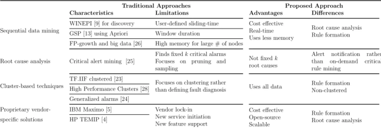
Compared to the mentioned works, the main contribution of this thesis is to create alarm rules to identify root causes by developing a system that combines a streaming big data infrastructure, a dynamic index for matching active alarms, an algorithm for generating candidate alarms, and a sliding-window based approach to save system resources. Table 1.1 gives main alarm correlation models for the considered problem, highlighting some of the most relevant work for each problem, while situating the contributions of this work.
Traditional Approaches Proposed Approach Characteristics Limitations Advantages Differences Sequential data mining
WINEPI [9] for discovery User-defined sliding-time Cost effective Real-time Uses less memory
Root cause analysis Rule formation GSP [13] using Apriori Window duration
FP-growth and big data [26] High memory for large # of nodes Root cause analysis
Finds fixed k critical alarms Focuses on pruning and sampling
Not fixed k root causes
Alert notification rather than on-demand critical rule mining
Critical alert mining [25] Cluster-based techniques
TF.IIF clustered [23]
Focuses on clustering rather
than defining fault diagnosis Uses all data
Rule formation Non-clustered High Performance Clusters [28]
Generalized alarms [24]
Proprietary vendor- IBM Maximo [5] Vendor lock-in New service initiation New feature support
Cost effective Open-source Scalable
Rule formation Root cause analysis specific solutions HP TEMIP [4]
Table 1.1: A comparison of various alarm correlation techniques applied for mo-bile operator networks
The rest of this thesis is organized as follows. Chapter 2 defines the method-ology. Chapter 3 presents the infrastructure of utilized platform. Chapter 4 presents the experience with the rule mining algorithm. Chapter 5 contains con-cluding remarks.
Finally, the main contributions of this thesis are as follows: • A rule mining algorithm is proposed to create alarm rules.
• A probabilistic candidate rule filtering is proposed to save system resources. • A root cause algorithm is proposed to find influential alarms in the system.
Chapter 2
Methodology
A large mobile telecommunications provider needs an intelligent alarm manage-ment platform. Such a platform would collect event data related to alarms and perform alarm analysis on this data to mine alarm rules and determine influen-tial alarms. In this thesis, the ALACA platform is utilized to handle performing alarm analysis. The ALACA platform relies on a big data architecture to store alarm event data, a stream processing module for complex event analysis, a root cause analysis module to mine alarm rules and detect influential alarms which is developed with the help of this thesis, and finally a web client for end-user interaction. We present the ALACA platform’s architecture later in Chapter 3.
In this chapter, the alarms and rules used in this work are formally described. The semantics of our rules by formulating the matching between a rule and an alarm sequence are formalized. The support and confidence requirements of the rules are given. Finally, the proposed rule mining algorithm, including a proba-bilistic filtering technique that significantly reduces the algorithm’s memory re-quirement and improves its running time performance is described.
The following conventions throughout the thesis with respect to notation is used: Symbols in regular font represent scalars, whereas those in boldface font represent vectors. Sets are denoted by upper-case calligraphic symbols.
2.1
Formalization
Each alarm has a kind and a time interval during which it was active. For
example, an alarm can be specified as A = (X, [t0, t1]). Here, X is the alarm
kind and [t0, t1] is the time interval during which the alarm was active. The start
time sorted list of all alarms is denoted as D. The alarm kind for an alarm A is denoted as A.k and the set of all alarm kinds as K = {A.k : A ∈ D}. The alarm
interval is denoted as A.i. The start time of the alarm interval is denoted as A.ts
and the end time as A.te. Sorted alarms of kind k are denoted as L.
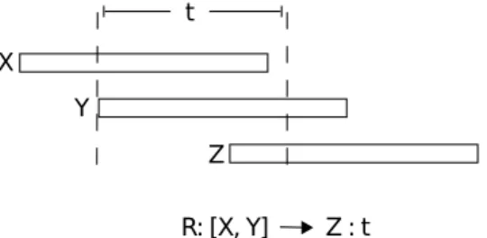
Alarm rules are defined as logical implications, where the antecedent is an ordered set of alarm kinds and the consequent is a single alarm kind. Each alarm rule is also associated with a time duration. For instance, a rule can be specified as R = [X, Y ] → Z : t. Here, there are two alarm kinds, namely X and Y , appearing as an ordered set on the antecedent, and there is a single alarm kind Z appearing as the consequent. Time duration, t, is given as the rule duration.
X Y
Z
R: [X, Y] Z : t t
Figure 2.1: An example sequence of events that match a given rule. The meaning of an alarm rule is as follows: When the alarms specified on the antecedent occur in order, then the alarm specified on the consequent is expected to occur within t time units. As an additional requirement, the intervals of all the alarms involved in a rule should intersect. For instance, in the running example, first X should start. Then Y should start before X ends. Then the rule predicts that, after Y starts, Z is expected to start within t time units, before X and Y end. For a rule R, we denote the antecedent as R.a and the consequent as R.c. The duration of the rule is denoted by R.d. The consequent cannot be contained in the antecedent, that is R.c 6∈ R.a. Fig. 2.1 illustrates a sequence of events matching a rule.
Formally, a set of events ordered by their start time, denoted as U , match a rule R, based on the following definition of a Boolean match function:
match(R, U ) ≡ ∩
A∈UA.i 6= ∅ ∧
[A.k : A ∈ U ] = R.a ∪ [R.c] ∧ U[−1].ts− U[−2].ts ≤ R.d
(2.1)
In Equation (2.1), there are three conditions: First condition requires that the intersection of the alarm intervals in U cannot be an empty set. Second condition requires that the set of all alarm kinds in U should be equal to the union of the alarm kind set of the rule’s antecedent alarm kinds set and the
consequent alarm kind. [j] notation is used to index the time ordered event set,
where an index j = −1 represents the last item and -2 the penultimate one. Final condition requires that the difference between the last item’s start time in U and the penultimate item’s start time should be less than or equal to the rule R’s duration. Therefore, for a rule match, these three conditions of (2.1) should be true.
2.2
Mining Alarm Rules
In order to mine alarm rules from a data set of alarms, a scalable rule mining algorithm is developed. The algorithm can mine rules in the format outlined so far, which additionally satisfy given confidence and support requirements. The algorithm can also be trivially adapted to mine rules where the antecedent is an
unordered set. The support threshold is denoted as τs ∈ N+ and the confidence
threshold as tc ∈ (0, 1]. To satisfy the support requirement, there must be at least
τs distinct event sub-sequences in the data set that match the rule. To support
the confidence requirement, at least tcfraction of the event sequences that match
the antecedent part of the rule must be followed by an addition event that results in the extended sequence matching the entire rule.
time ordered set of all events:
support(R, D) = |{U ⊆ D : match(R, U )}| (2.2)
The confidence of a rule is formally defined as follows: conf idence(R, D) = support(R, D) /
|{U ⊆ D : ∩
A∈UA.i 6= ∅ ∧ [A.k : A ∈ U ] = R.a}|
(2.3)
Before the rule mining algorithm is applied, the alarm data set is taken through a pre-processing, which is detailed next.
2.3
Alarm Pre-processing
Algorithm 1: Alarm pre-processing. Input: D, Sorted alarms; K, Alarm kinds
Output: C, Pre-processed alarms; I, Interval index
1 M ← {u 7→ L : u ∈ K ∧ L = {A ∈ D : A.k = u}};
2 for u 7→ L ∈ M do
3 n ← 0;
4 for i ∈ [1..|L|) do // in start time order
5 if L[i].ts < L[n].te then 6 if L[i].te > L[n].te then 7 L[n].i = [L[n].ts, L[i].te]; 8 else 9 n ← n + 1; 10 L[n] ← L[i]; 11 L ← L[0..n]; 12 C ← sort(∪u7→L∈ML, 7→ .ts);
13 I ← build interval index(C);
The pre-processing phase is used to cleanse the alarm data set and to index the alarms. The cleansing involves merging alarms of same kind whose time intervals intersect and ordering the resulting alarm data set based on start time. Indexing involves creating an interval tree using the alarm intervals. The interval tree [29]
enables querying the alarm data set using a query time point. In particular, it can retrieve the alarms whose time intervals contain the query time point in O(log(n)) time, where n is the number of alarms. An interval index can be constructed in O(n · log(n)) time. Algorithm 1 describes the pre-processing step.
2.4
Rule Detection
MineAlarmRules procedure, given in Algorithm 2, describes how alarm rules are detected. First, alarms are partitioned based on their kinds. Then for each alarm kind, a set of candidate rules are found whose consequent is the given alarm kind (line 4). This is done via the MineAlarmRulesForKind procedure. The set of candidate rules found this way satisfies the support requirement, but may not satisfy the confidence requirement. Thus, the candidate rules go through a filtering process (line 5). This is done via the EnforceConfidences algorithm. The filtering process removes the candidate rules that do not meet the confidence criteria. Merging rules generated for different alarm kinds produces the final set of rules.
Algorithm 2: MineAlarmRules algorithm
Input: C, Pre-processed alarms; I, Interval index; τs, Support threshold;
τc, Confidence threshold
Output: R, Mined alarm rules
1 R ← ∅;
2 M ← {u 7→ L : u ∈ K ∧ L = {A ∈ C : A.k = u}};
3 for u 7→ L ∈ M do
4 V ← MineAlarmRulesForKind(L, I, τs);
5 R ← R ∪ EnforceConfidences(V, C, I, τc);
MineAlarmRulesForKind procedure, given in Algorithm 3, describes how alarm rules for a given alarm kind are detected. A quick check is first done to see whether the number of alarms of the given kind is at least equal to the support threshold. If not, enough occurrences cannot be acquired for a rule whose consequent is of the given kind. Thus the algorithm is simply returned in this case. Otherwise, in order to determine the candidate rules, the alarms of the given
kind are iterated. This time ordered alarm list is already computed earlier, and is the parameter L to the algorithm in the pseudo-code. For each alarm in this list, referred to as an anchor alarm, a number of candidate rules are generated (line 5). These candidate rules have the important property that for each one there is a matching alarm subsequence terminating at the anchor alarm. The candidate rules are found via the GetCandidateRules procedure. A map is used, M in the pseudo-code, to keep a count of the number of times each candidate rule has appeared as iteration through the anchor alarms and generate candidate rules. Two candidate rules returned by different calls to GetCandidateRules are considered the same if their antecedents are the same (their consequent are the same by construction). They may differ in their duration. The maximum duration is taken as the duration of the candidate rule kept in the map for counting the occurrences. Alternatively, a statistical choice could be made, such as maintaining a running mean and average duration and at the end determining the duration value that corresponds to the 95% percentile assuming a normal distribution. At the end of the process, The candidate rules whose occurrence counts are greater than or equal to the support threshold are only kept.
Algorithm 3: MineAlarmRulesForKind algorithm
Input: L, Sorted alarms of kind u; I, Interval index; τs, Support threshold
Output: R, Candidate alarm rules
1 R ← ∅;
2 if |L| < τs then return;
3 M ← ∅; // map of candidate rules
4 for A ∈ L do 5 for R ∈ GetCandidateRules(A, I) do 6 if R.a ∈ M then 7 Let M [R.a] = (R0, s); 8 R.d ← max(R.d, R0.d); 9 M [R.a] ← (R, s + 1); 10 else 11 M [R.a] ← (R, 1); 12 for K 7→ (R, s) ∈ M do 13 if s ≥ τs then 14 R ← R ∪ R;
list of candidate rules for a particular anchor event is generated. These candidate rules are the ones for which there exists a matching alarm subsequence terminat-ing at the anchor event. For this purpose, the interval tree with the start time of the anchor event is queried and all other events that are active at that time is found. The result is a subset of events ordered based on their start time. Any start time ordered subset of these rules can serve as the antecedent of a candi-date rule. Thus, one candicandi-date rule for each such subset is generated, with the duration set to the time difference between the start times of the last event in the subset and the anchor event.
Algorithm 4: GetCandidateRules algorithm Input: A, Alarm; I, Interval index
Output: R, Candidate alarm rules
1 R ← ∅;
2 V ← ∅;
3 for A0 ∈ I.lookup(A.ts) do
4 if A0.ts 6= A.ts and A0.te 6= A.ts then
5 V ← V ∪ {A0};
// For time ordered subsets of the antecedents
6 for U ⊂ V do
7 if |U | = 0 then continue;
8 t ← A.ts− U[−1].ts;
9 R ← [A0.k : A0 ∈ U ] → A.c : t;
10 R ← R ∪ {R};
Finally, EnforceConfidences procedure, given in Algorithm 5, describes how the short list of candidate alarms is filtered to retain only the ones that satisfy the confidence requirement. For this purpose, the confidence of each rule is computed. The last element of the rule’s antecedent is used to iterate over all the events of that kind. Each one of these events represent a possible point of match for the rule’s antecedent. Let us call these events vantage events. A vantage event’s start time is used to query the interval index and all other events that are active during that time are found. The results from querying the interval tree in start time order are iterated and whether a sequence of events whose kinds match the rule’s antecedent up to and excluding its last item can be found is checked. If so, then an antecedent match at this vantage event is had and the
match may correspond to a rule match or not. To check that, whether there is an event whose kind matches that of the rule consequent is simply found out. The search is limited to events that start after the leverage event within the
rule’s duration. Also, it should start before any of the events matching the
antecedent finish. If a rule match is found, then the corresponding counter, nt
in the pseudo-code, is incremented. Accordingly, nt/ns gives us the confidence,
which is compared against the confidence threshold, τc, to perform the filtering.
Algorithm 5: EnforceConfidences algorithm
Input: V, Candidate rules; C, Pre-processed alarms; I, Interval index; τc,
Confidence threshold Output: R, Alarm rules
1 R ← ∅;
2 for R ∈ V do
3 ns ← 0; nt← 0;
4 for i ∈ [0..|C|) do
5 if C[i].k 6= R.a[−1] then continue;
// check antecedent alarms
6 j ← 0; t ← C[i].te;
7 for A ∈ I.lookup(C[i].ts) do
8 if R.a[j] = A.k then
9 j ← j + 1;
10 t ← min(t, A.te);
11 if j 6= |R.a| − 1 then continue;
12 ns ← ns+ 1;
// check consequent alarm
13 for l ∈ [i + 1..|C|) do 14 if C[l].ts> C[i].ts+ R.d or C[l].ts >= t then 15 break 16 if C[l].k = R.c then 17 nt ← nt+ 1; 18 break 19 if nt/ns≥ τc then 20 R ← R ∪ {R};
2.5
Probabilistic Candidate Rule Filtering
A downside of our rule mining algorithm is that the memory usage can go up significantly, since many candidate rules are maintained in Algorithm 3 with very low occurrence counts, that are eventually discarded due to failing the support requirement. This may prevent the algorithm scaling to large alarm data sets. To solve this problem, a probabilistic filtering algorithm is developed. The funda-mental idea behind the filtering algorithm is that, if the current occurrence count of a rule is very low compared to the expected occurrence count to eventually pass the support threshold assuming a uniform distribution of occurrences over the alarm set, then that candidate rule can be discarded right away. This filtering concept is mathematically formalized.
Let Sn be a random variable representing the number of occurrences of a
candidate rule after observing n anchor events. Occurrence of a rule for the ith
event is a Bernoulli random variable, denoted as Xi, is assumed. To have enough
support in the average case, E[Xi] ≥ τs/N, ∀i is need to be had, where N is
the total number of anchor events (|L| in the pseudo-code). Sn =
PN
i=1Xi and
E[Sn] = n · τs/N are had. The probabilistic candidate rule filtering works by
discarding a candidate rule if after observing n anchor events Sn is less than k
and P r(Sn≤ k) ≤ 1 − φ, where φ ∈ [0, 1] is a configuration parameter called the
filtering confidence. φ is typically close to 1.
Based on the Chernoff-Hoeffding bound [30], we have: P r(Sn ≤ (1 − δ) · E[Sn]) ≤ e−δ
2·E[S
n]/2 (2.4)
Matching this formula with our filtering condition of P r(Sn ≤ k) ≤ 1 − φ, we
get:
k = n · τs/N −p−2 · n · τs/N · log (1 − φ) (2.5)
The map from Algorithm 3 is replaced with an ordered tree using the occur-rence count for ordering the candidate rules to implement probabilistic candidate rule filtering. Then after processing each anchor event, any candidate rules whose
occurrence count is less than or equal to k are removed with iteration over this tree. Note that k is updated after processing each candidate rule.
In this chapter, the terminology is defined, Alarms, Rules, and Rule Mining and the methodology is given. First, what an alarm and what a rule means, as well as what the components and requirements of an alarm and a rule are formally defined. Second, the rule mining algorithm is formally defined, in a step-by-step manner. Finally, a probabilistic filtering technique for reducing the system resources used for mining rules was proposed, in order to make the mining algorithm fast.
Chapter 3
ALACA: Scalable and Real-time
Alarm Data Analysis
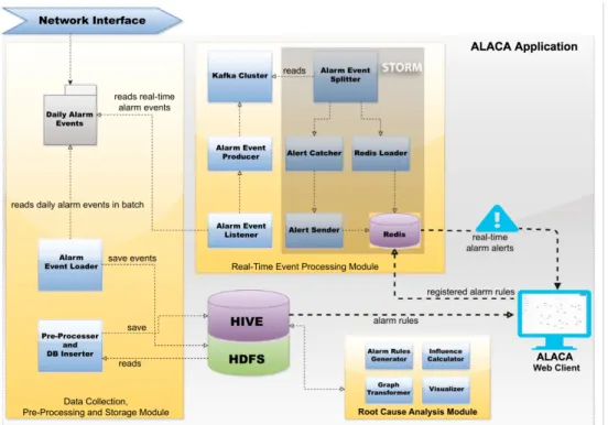
ALACA is a platform to process vast amounts of alarms where a demo version is demonstrated in the paper of [1]. These alarms are collected from different sources in real-time and identify the root causes of problems. The platform is composed of three main modules: (a) Data Collection, Pre-prosessing, and Storage; (b) Real-time Alarm Data Processing; and (c) Root Cause Analysis which is improved by the help of this thesis. Fig. 3.1 [1] indicates the infrastructure of the platform. The Data Collection, Pre-prosessing, and Storage module collects and transforms
data into a suitable format for further analysis and stores. The Root Cause
Analysis module executes the proposed scalable rule and graph mining algorithm for root cause analysis on alarm events. The Data Collection module feeds the Root Cause Analysis module with the required alarm data. The rules discovered by the Root Cause Analysis module are registered into the Real-time Alarm Data Processing module. The modules are briefly explained in next sections.
Figure 3.1: High level architecture of ALACA platform. Adapted from Streaming alarm data analytics for mobile service providers, by E. Zeydan, U. Yabas, S. Sozuer, and C. O. Etemoglu, 2016, NOMS 2016 - 2016 IEEE/IFIP Network Operations and Management Symposium, pp. 1021 - 1022. Copyright [2016] by IEEE. Adapted with permission.
3.1
Data Collection, Pre-Processing, Storage
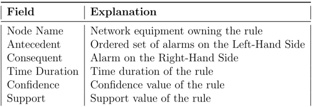
For representing real-time alarms, Event Data Type is used. It includes the fields such as Node Name, Alarm Name, Event Time and Severity as shown in Table 3.1. For alarm data processing, Alert Data Type models the alarm warnings sent back into user in real-time. This alert type includes alarm information that can happen in the future. Its contents are listed in Table 3.2. Rule Data Type includes rules that are pre-calculated and pre-registered into the ALACA’s CEP module. Using this rule model, warnings or alarm alerts are sent back to the users. The details are in Table 3.3.
The alarm information is collected and stored in the network operations cen-ter. The kind of network status information stored and its format depends on
many factors, such as configuration, type, and vendor of the nodes and network equipment. As shown in Fig. 3.1, the Data Collection, Pre-Processing and Stor-age module contains the three components: Alarm Event Loader, Pre-processor, Database Inserter whose details are given in the demonstration paper [1].
Field Explanation
Node Name Network equipment producing the alarm
Alarm Name Name identifying the alarm kind
Event Time Time duration of the alarm
Severity Priority state of the alarm
Table 3.1: Alarm Event data format.
Field Explanation
Node Name Network equipment producing the alarm
Alarm Names List of possible alarms that can occur
Time Difference Calculated time interval between the occurring alarms
Captured Time Required time for the alert data model to be formed in the system
Estimated Occurrence Time The information about alarms generation time
Table 3.2: Alarm Alert data format.
Field Explanation
Node Name Network equipment owning the rule
Antecedent Ordered set of alarms on the Left-Hand Side
Consequent Alarm on the Right-Hand Side
Time Duration Time duration of the rule
Confidence Confidence value of the rule
Support Support value of the rule
Table 3.3: Alarm Rule data format.
3.2
Real-Time Alarm Data Processing
The Real-time Alarm Data Processing module collects, distributes alarm data and makes complex event analysis on this data, assist the users in seeing the real-time alarm flow with low-latency. It contains the following components: Alarm Event Listener, Alarm Event Producer, Kafka Cluster, Alarm Event Splitter, Re-dis Loader whose details are given in the demonstration paper [1]. There are
two additional components which are about alert notification. Alarm Catcher, which runs pre-registered rules over alarm data coming from AlarmLog Splitter in Event data format. Registered rules are modeled using the Rule data format. This module performs the calculation based on a window of size τ with a slice of α. This means that last τ time units worth of alarm data are processed against the rules every α time units. If after processing the alarms, a future alarm is predicted to occur based on the rules, these warnings are sent in the Alert data format to the Alert Sender module for further processing. Alert Sender, which writes Alert data coming from Alert Catcher module into the database. Alert Sender will not write into the database if an alert is already available in the database or if its estimated occurrence time has passed.
3.3
Root Cause Analysis
The frequently occurring alarm rules are transformed into a graph representation, which is further utilized in the system for root cause analysis and visualization. These rules are identified by a four phase algorithm: alarm cleansing, alarm indexing, i.e. Algorithm 1: Alarm pre-processing for both pre-processing and building interval indexes, rule generation, and rule elimination i.e. Algorithm 2: for both alarm rule generation and eliminations. In summary, in the cleansing phase, alarms with matching kinds whose time intervals overlap are merged. In the indexing phase, an interval index is built over the alarms, such that the list of alarms that are active at a given time can be found quickly (in logarithmic time). In the rule generation phase, candidate alarm rules are generated for each possible consequent alarm. For this purpose, for each alarm X found in the alarm sequence, the set of active alarms when X has started is found using the interval index. Then, candidate rules are created with X on the consequent and subsets of the found alarms on the antecedent. Occurrence counters are maintained for these candidate rules across all X appearances. After all Xs are processed, the elimination phase starts. The candidate rules with low support or confidence values are eliminated. Here, the support value is the minimum occurrence count
for a rule to be retained. And the confidence value is the prediction accuracy the rule has (how frequent the consequent holds when the precedent does).
The alarm rules identified as above are then transformed into a directed graph hV, Ei, where vertexes V are the alerts and the edges E are the rule relationships between them. For example, if two rules are calculated for a network equip-ment, such as [A, B] → C and [D, E] → B, then the vertex set becomes V = {A, B, C, D, E} and the edge set becomes E = {(A, C), (B, C), (D, B), (E, B)}. Graphs for unique network equipment types or the entire system can be gener-ated. Based on the graph representation, root-cause alarms are identified by a scoring mechanism. After calculating the scores of all alarms, most influential alarms are detected as the ones with the top influence scores.
Algorithm 6: Score algorithm calculates each alarm’s influence score Input: A directed graph, G(V,E)
1 foreach Vi in G do
2 if Vi is a leaf node then
3 Vi.s ← 0;
4 else
5 Vi.s ← 1+sum(Vij.s | Vij is an out neighbor of Vi)/2;
The alarm influence score calculation is performed as follows: First, for each network equipment (i.e. Node Name in Table 3.1) that generates alarms, a com-posite graph is created by combining the rules mined for that equipment. Then this composite graph is topologically sorted. Next, vertexes of the graph are pro-cessed in reverse topological order and scored by Algorithm 6. When a composite graph is fully processed, each vertex, and thus each unique alarm kind that ap-pears in the graph, accumulates some number of points. To compute the global influence of an alarm, we sum up all the points it has accumulated across all composite graphs.
To sum up, the details of the ALACA platform with its three main modules are presented: Data Collection, Pre-Processing and Storage, Root Cause Analysis and Real-Time Event Processing. Data Collection, Pre-Processing and Storage Module collects alarm events and loads them into Hadoop Distributed File Sys-tem (HDFS) while performing filtering, cleaning and parsing of raw data from
HDFS, and stores the cleansed data. Root Cause Analysis Module creates alarm rules, transforms them into a graph representation, calculates influence scores from graphs, and visualizes those graphs. Real-Time Event Processing Module reads real-time alarm data from the sources and prepares the alarm data for the Data Collection, Pre-Processing and Storage Module, CEP, and the ALACA Web Client.
Chapter 4
Experiments
In this chapter, the experimental data set, the experiments and the performance results of the proposed solution are presented. First of all, the proposed solution is compared with a traditional sequence mining algorithm. After this, three main
parameters are used for our evaluation. The first one is the confidence (τc) as given
in Equation 2.3. The second is the support (τs) as given in Equation 2.2. The
third is the filter confidence (k), as given in Equation 2.5. The general purpose is to see the impact of these parameter values on rule counts, running time, and memory usage. All the experiments are run three times and the average values are reported as results. Finally, the root-cause analysis results are also shown.
4.1
Experimental Setup
The experimental data set is obtained from a major telecom provider in 2012. The data have a total of 2,054,296 pre-processed alarm events, which are produced by 80,027 different nodes. For experiments, the data set is splitted into 250K, 500K, 750K, 1M, 1.25M, 1.5M, 1.75M, and 2M instances by ordering them by
event time. The experiments are run on a workstation which has 128GB of
is used to process data. First, memory usage was attempted to measure for each experiment in terms of the number of bytes. However, due to the garbage collection of the JVM, memory measurements did not produce healthy results. Instead, the maximum candidate rule map size as given in Algorithm 3 is used for capturing the memory usage. For each experiment, the running time is reported as maximum, minimum, and average over different nodes.
4.2
Comparison of Proposed and RuleGrowth
-Sequential Rule Mining Algorithm
Before presenting the experiments on the impact of major workload and sys-tem parameters, the proposed algorithm is compared with a traditional sequen-tial data mining algorithm, RuleGrowth [31]. For this evaluation, a prediction-occurrence model with the alarm rules is implemented as the formation is defined in Section 2. This model is based on the rule occurrences on the transactions. If the antecedent alarms of the sequential rule of a node occurs in a transaction, then the prediction ”the consequent alarm of this rule will also occur in this transac-tion” is made. If this consequent one also occurs, the prediction is correct. Then, the correctness of the prediction is calculated as accuracy. The alarm rules are mined from data set (alarm count: 369,345) which are dated from 10/08/2012 to 23/08/2012 based on the Nokias radio access network logs with support value of 10 and confidence value of 0.9. The prediction accuracy is created from these logs (alarm count: 27,855) on 24/08/2012. As shown in Table 4.2, the RuleGrowth algorithm makes 2,702 predictions and 864 rule occurrences take place based on these predictions in this experiment. Therefore, its accuracy is around 32.0%. The proposed algorithm makes 366 predictions where 266 of them has occurred. Hence, the accuracy becomes 72.7%. In the experiments, the RuleGrowth al-gorithm made many predictions while it consumes a lot of resources and time. These results indicate that the proposed method makes more accurate predictions by using less resources and time.
The results for the current experiment are given in Table 4.2. Prediction Count is the number of the antecedent alarms of a sequential rule occurrences on the transactions, and Rule Occurrence Count is the number of the consequent alarms of the rule following the antecedents occurrences on the transactions. Accuracy is defined as the rule occurrence counts over prediction counts for transactions in order to measure how correct is the prediction. Recall value is defined as the ratio of rule occurrence counts which are calculated by considering only training data and both training and test data respectively. The proposed solution makes 2.27 times better predictions than RuleGrowth algorithm.
Algorithm Prediction Count Rule Occurrence Count Accuracy Recall
RuleGrowth 2,702 864 32.0 % 69.8%
Proposed method 366 266 72.7 % 86.4%
Table 4.1: Results of prediction-rule model for sequential rules and the proposed Algorithm 3
4.3
Impact of Confidence
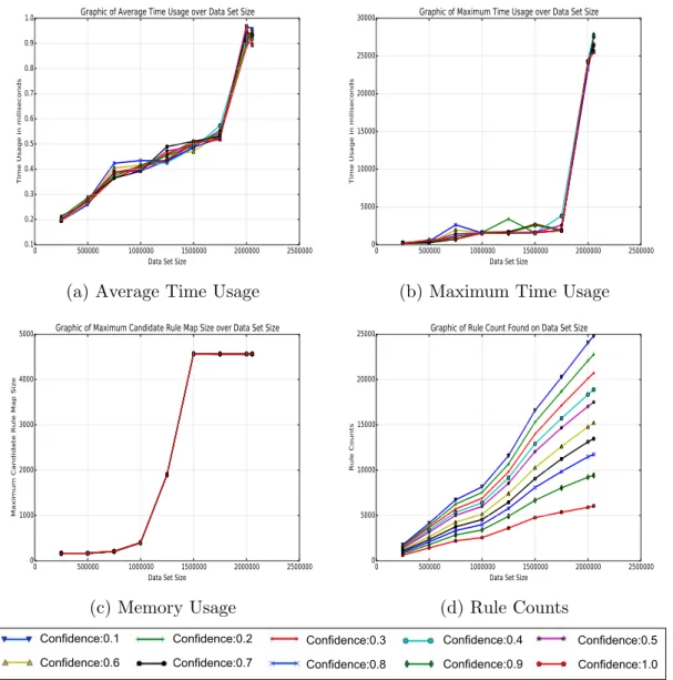
First parameter experiment is made on confidence value as it changes between 0.1 and 1.0. Fixed support value of 10 and fixed filter confidence value of 0.9 are used. Rule counts, maximum candidate rule size, time max., min., avg. are measured over data set size. Since the rules are mined as node based, maximum candidate rule map size as given in Algorithm 3 is used for memory usage and time is observed as maximum, minimum and average. Fig. 4.1 shows the results of different confidence values over data set size. Data set size is on the x -axis of all plots. Time usage in milliseconds is on the y-axis of Fig. 4.1.a and Fig. 4.1.b. Maximum candidate rule map size is given on the y-axis of Fig. 4.1.c and rule counts are given on the y-axis of Fig. 4.1.d. Different confidence values are the lines on the plots as given on the legend.
There is a linear relation between data set size and time usage in Fig. 4.1.a and Fig. 4.1.b for this experiment. However, there is no relation between confidence value and memory in Fig. 4.1.c. It’s because candidate rules are firstly created and
the confidence values are calculated then finally whether they hold the threshold value is checked. That’s the same reason of time usages are almost the same of all confidence levels. In all data sets, the minimum time usage is almost 0, so we didn’t give the minimum time usage plot. Fig. 4.1.d shows the rule counts created for each data set and each confidence level. It shows how the confidence value works on the each data set size. If the confidence value is maximum level, 1.0, the rule counts are minimum for all data sets, and vice versa. For instance, the rule count is 6041 when the confidence level is 1.0 for using all data, although the rule count is 24817 when the confidence level is 0.1.
0 500000 1000000 1500000 2000000 2500000
Data Set Size 0.1 0.2 0.3 0.4 0.5 0.6 0.7 0.8 0.9 1.0
Time Usage in miliseconds
Graphic of Average Time Usage over Data Set Size
(a) Average Time Usage
0 500000 1000000 1500000 2000000 2500000
Data Set Size 0 5000 10000 15000 20000 25000 30000
Time Usage in miliseconds
Graphic of Maximum Time Usage over Data Set Size
(b) Maximum Time Usage
0 500000 1000000 1500000 2000000 2500000
Data Set Size 0 1000 2000 3000 4000 5000
Maximum Candidate Rule Map Size
Graphic of Maximum Candidate Rule Map Size over Data Set Size
(c) Memory Usage
0 500000 1000000 1500000 2000000 2500000
Data Set Size 0 5000 10000 15000 20000 25000 Rule Counts
Graphic of Rule Count Found on Data Set Size
(d) Rule Counts
Confidence:0.1 Confidence:0.6
Confidence:0.2 Confidence:0.3 Confidence:0.4 Confidence:0.5 Confidence:0.7 Confidence:0.8 Confidence:0.9 Confidence:1.0
4.4
Impact of Support
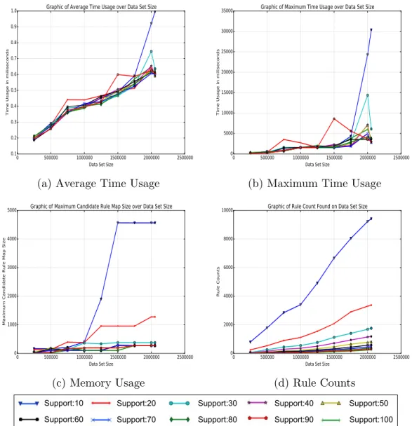
The next experiment is on support value as it changes between 10 to 100. Fixed confidence and filter confidence values of 0.9 are used. Rule counts, maximum candidate rule size, time max., min., avg. are measured as well. Fig. 4.2 shows the results of different confidence values over data set size. Data set size is on the x -axis of all plots again. Time usage in milliseconds is on the y--axis of Fig. 4.2.a and Fig. 4.2.b. Maximum candidate rule map size is given on the y-axis of Fig. 4.2.c and rule counts are given on the y-axis of Fig. 4.2.d. Different support values are the lines on the plots as given on the legend.
0 500000 1000000 1500000 2000000 2500000
Data Set Size 0.1 0.2 0.3 0.4 0.5 0.6 0.7 0.8 0.9 1.0
Time Usage in miliseconds
Graphic of Average Time Usage over Data Set Size
(a) Average Time Usage
0 500000 1000000 1500000 2000000 2500000
Data Set Size 0 5000 10000 15000 20000 25000 30000 35000
Time Usage in miliseconds
Graphic of Maximum Time Usage over Data Set Size
(b) Maximum Time Usage
0 500000 1000000 1500000 2000000 2500000
Data Set Size 0 1000 2000 3000 4000 5000
Maximum Candidate Rule Map Size
Graphic of Maximum Candidate Rule Map Size over Data Set Size
(c) Memory Usage
0 500000 1000000 1500000 2000000 2500000
Data Set Size 0 2000 4000 6000 8000 10000 Rule Counts
Graphic of Rule Count Found on Data Set Size
(d) Rule Counts
Support:10 Support:60
Support:20 Support:30 Support:40 Support:50
Support:70 Support:80 Support:90 Support:100
There is a linear relation between data set size and time usage in Fig. 4.2.a and Fig.4.2.b as well as previous experiment. Additionally, Fig. 4.2.c shows that there is a opposite relation between support value and memory usage. While the support value increases, the memory usage decreases. The dramatic change on the memory between support values 10 and 20 is observed. For the data set size 1.25M, the candidate rule map size is 1899 for the support value 10 and 956 for the support value 20. For huger data sets, this change is getting bigger. For the data set size 2M, the candidate rule map size is 4564 for the support value 10 and 1277 for the support value 20. We see the rule counts in Fig. 4.2.d. There is a reverse parabolic relation between rule counts and support values. When the support value increases, the rule counts dramatically decreases. Although there are 9418 rules created for all instances with the support value 10, there are 3375 rules created with the support value 20.
4.5
Impact of Filter Confidence
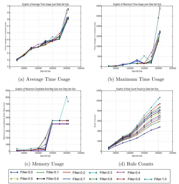
The next experiment is on filter confidence as it changes between 0.0 to 1.0. Fixed confidence value of 0.9 and fixed support value of 10 are used. Filter confidence 0.0 assumes that the data set is perfectly uniform, 1.0 assumes that the data is not uniform at any point. Rule counts, maximum candidate rule size, time max., min., avg. are measured as previous experiments. Data set size is on the x -axis of all plots of Fig. 4.3. Time usage in milliseconds is on the y-axis of Fig. 4.3.a and Fig. 4.3.b. Maximum candidate rule map size is given on the y-axis of Fig. 4.3.c and rule counts are given on the y-y-axis of Fig. 4.3.d. Different filter confidence values are the lines on the plots as given on the legend.
There is linear relation between data set size and time usage which can be seen in Fig. 4.3.a and Fig. 4.3.b as expected. The filter confidence effect on the time usage can be observed by dramatic change between 0.8 and 1.0 in these figures. The maximum time is 16945 ms when the all data processed with the filter confidence level 0.8. However, the maximum time is 29488 ms when the all data processed with the filter confidence level 1.0. The same effect on the
memory can be seen in Fig. 4.3.c. While the maximum candidate rule map size is 4564 with filter confidence level 0.9, it is 7392 with filter confidence level 1.0 for the all data. The rule counts over data size for each filter confidence levels are given in Fig. 4.3.d. In small data sets, the rule counts can be acceptable at any filter confidence levels. On the other hand, the rule counts are reasonable at filter confidence levels 0.8 and 0.9 for big data sets.
0 500000 1000000 1500000 2000000 2500000
Data Set Size 0.1 0.2 0.3 0.4 0.5 0.6 0.7 0.8 0.9 1.0
Time Usage in miliseconds
Graphic of Average Time Usage over Data Set Size
(a) Average Time Usage
0 500000 1000000 1500000 2000000 2500000
Data Set Size 0 5000 10000 15000 20000 25000 30000
Time Usage in miliseconds
Graphic of Maximum Time Usage over Data Set Size
(b) Maximum Time Usage
0 500000 1000000 1500000 2000000 2500000
Data Set Size 0 1000 2000 3000 4000 5000 6000 7000 8000 9000
Maximum Candidate Rule Map Size
Graphic of Maximum Candidate Rule Map Size over Data Set Size
(c) Memory Usage
0 500000 1000000 1500000 2000000 2500000
Data Set Size 0 2000 4000 6000 8000 10000 12000 Rule Counts
Graphic of Rule Count Found on Data Set Size
(d) Rule Counts
Filter:0.0 Filter:0.5
Filter:0.1 Filter:0.2 Filter:0.3 Filter:0.4
Filter:0.6 Filter:0.7 Filter:0.8 Filter:0.9 Filter:1.0
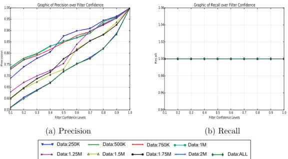
Figure 4.3: Graphics of Different Filter Confidence Values over Data Set Size Fig. 4.4 shows precision and recall values of rules. On the x -axis, there are filter confidence level values. Data set sizes are the lines for these plots as given
on the legend. Precision value is given on the y-axis of Fig. 4.4.a and recall value is given on the y-axis of Fig. 4.4.b. Filter confidence levels 0.8 and 0.9 give reasonable precision values for each data set. For instance, when the data set size is 250K, the precision value is 0.944 for the filter confidence level 0.8. For the same filter confidence level, the precision value is 0.821 when the all data are used. Since no different rules are created when filter confidence values change, all recall values are 1.0 which is given in Fig. 4.4.b. So, the f-values are the same with precision values that’s why the f-measure plot is not given.
0.1 0.2 0.3 0.4 0.5 0.6 0.7 0.8 0.9 1.0
Filter Confidence Levels 0.55 0.60 0.65 0.70 0.75 0.80 0.85 0.90 0.95 1.00 Precision
Graphic of Precision over Filter Confidence
(a) Precision
0.1 0.2 0.3 0.4 0.5 0.6 0.7 0.8 0.9 1.0
Filter Confidence Levels 0.94 0.96 0.98 1.00 1.02 1.04 1.06 Recall
Graphic of Recall over Filter Confidence
(b) Recall
Data:250K
Data:1.5M
Data:500K Data:750K Data:1M
Data:1.25M Data:1.75M Data:2M Data:ALL
Figure 4.4: Precision and Recall Graphics of Different Filter Confidence Values over Data Set Size
4.6
Alarm Impact
In order to compute the impact score of each alarm, first, the alarm rules are created from the experimental data set described in Section 4.1. Fixed confidence value of 0.9, fixed support value of 10 and fixed filter confidence value of 0.9 are used for alarm rule generation. At the end of the process, there are 9, 418 rules obtained from the data set. Then, based on the constructed rules, the rule graphs are created and the corresponding influence scores are calculated for each
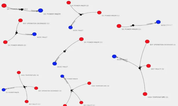
node. For instance, from Node Name DI2146 which corresponds to a BTS inside RAN, 8 alarm rules are created as shown in Fig. 4.5. The consequent alarm is represented as the blue vertex on an edge originating from a red vertex. To indicate the alert order in the rule, small labels are used to number the antecedent alarms. As a result, the rules can be easily read from the graphs. There are 6 unique alarms used in these rules. The influence scores which are calculated by using Algorithm 6 for these are also listed in Table 4.2.
FAULT
DEGRADED (2)
)
RE (3)
Figure 4.5: The alarm rules of Node Name DI2146’s node which corresponds to a BTS of RAN of MO.
Alarm Name Score
BCF OPERATION DEGRADED 1.00 BCF FAULTY 1.50 ACDC FAULT 0.00 DC POWER MAJOR 1.00 DC POWER MINOR 1.50 HIGH TEMPERATURE 1.75
Table 4.2: Influence Score of Alarms in the node DI2146.
The influence scores of alarms are calculated for root cause analyses by using Algorithm 6 for all nodes to identify alarm impact. Because the rule graphs are
created as node based, the maximum influence score is 1.875 for the alarm ”DC Power Minor”. We aggregate the scores to see root-causes in Fig. 4.6 as given most 15 influential alarm scores. There are alarm names on the x -axis and the aggregated scores on the y-axis. The most influential alarms are the alarm ”DC Power Minor” with score of 835.125 and the alarm ”DC Power Major” with score of 519.500. 0 100 200 300 400 500 600 700 800 900 DC PO WER MIN OR DC PO WER MAJO R ACDC FAUL T SHELT ER AIRC ONDIT ION MAIN S BRE AKDO WN WITH BATT ERY BA CK UP PCM FAILU RE SHELT ER DO OR OP EN CABIN ET O PEN WCD MA BA SE ST ATIO N OU T OF U SE BEAT ING B TS AL ARM FAILU RE IN SEND ING S YSTE M IN FORMA TION TO BT S SITE CONT INUO US RE START S OF B CF TRX HIGH T EMP ERATU RE FAILU RE IN WCD MA W BTS O M CO NNEC TION BATT ERY LO W Sc or e Alarm Impact
Figure 4.6: The Most 15 Influential Alarms Impact Scores
To sum up, the experiments are made on a real data set collected from a mobile network operator’s infrastructure to see the effects of our parameters and observe the most effective alarms that can be the root-cause of the subsequent alarms. Although the confidence value doesn’t affect the system resources, it affects the rule counts as expected. The support value have noticeable impact on the system resources used. The rule counts decrease dramatically when the support value increases. The final experiment are made on the filter confidence parameter to see the effect of our sliding-window based approach. When the filter confidence level is 0.8, the system resources are saved and the precision level is higher than 0.80 for all data sets, which is quite reasonable. The alarm “DC Power Minor” is more influential than the alarm “DC Power Major” and “ACDC Fault” which
coincides with the fact that before a major power shut down occurs at a given BTS, minor warnings arrive into network operation center of the mobile operator.
Chapter 5
Conclusion
This thesis introduces an alarm correlation method and root-cause analysis for alarms. These methods are applied to a real-time alarm data analytics platform by creating the root cause analysis module which is one of most critical modules of the platform. This platform is developed for a major mobile service provider. Both practical and theoretical contributions are provided on insights on large-scale alarm management and mining. The experiments show that the sliding-window based approach saves system resources by using a filter confidence level of 0.8 or 0.9, while maintaining the high precision of the alarm rules. The developed system is in active use within the network operation center of a major mobile telecom provider. Measuring the ticket reductions and the long-term cost savings for the network operator is planned as future work.
This work can be extended in several directions. The current system is devel-oped as node based. As a future work, the system performance can be improved by using clustered nodes and rules can be constructed using these clustered rules. This can result in detecting more influential alarm rules due to the addition of new rules. One can also extend the root cause analysis to be utilized for trend analysis of arriving alarms at a seasonal scale.
Bibliography
[1] E. Zeydan, U. Yabas, S. S¨oz¨uer, and C¸ . ¨O. Etemo˘glu, “Streaming alarm data
analytics for mobile service providers,” in Network Operations and Manage-ment Symposium (NOMS), 2016 IEEE/IFIP, pp. 1021–1022, IEEE, 2016. [2] H. Yan, L. Breslau, Z. Ge, D. Massey, D. Pei, and J. Yates, “G-rca: a generic
root cause analysis platform for service quality management in large ip net-works,” IEEE/ACM Transactions on Networking, vol. 20, no. 6, pp. 1734– 1747, 2012.
[3] H. Herodotou, B. Ding, S. Balakrishnan, G. Outhred, and P. Fitter, “Scalable near real-time failure localization of data center networks,” in Proceedings of the 20th ACM SIGKDD international conference on Knowledge discovery and data mining, pp. 1689–1698, ACM, 2014.
[4] “TeMIP Fault Management.” https://en.wikipedia.org/wiki/HP_
OpenView, 2016. [Online; accessed 30-September-2016].
[5] “Maximo Asset Management.” http://www-03.ibm.com/software/
products/en/maximoassetmanagement/, 2015. [Online; accessed
30-September-2016].
[6] I. Rouvellou and G. W. Hart, “Automatic alarm correlation for fault identifi-cation,” in INFOCOM’95. Fourteenth Annual Joint Conference of the IEEE Computer and Communications Societies. Bringing Information to People. Proceedings. IEEE, vol. 2, pp. 553–561, IEEE, 1995.
[7] S. Wallin, “Chasing a definition of alarm,” Journal of Network and Systems Management, vol. 17, no. 4, p. 457, 2009.
[8] E. P. Duarte, M. A. Musicante, and H. D. H. Fernandes, “Anemona: a programming language for network monitoring applications,” International Journal of Network Management, vol. 18, no. 4, pp. 295–302, 2008.
[9] H. Mannila, H. Toivonen, and A. I. Verkamo, “Discovery of frequent episodes in event sequences,” Data mining and knowledge discovery, vol. 1, no. 3, pp. 259–289, 1997.
[10] M. Klemettinen, H. Mannila, and H. Toivonen, “Rule discovery in telecom-munication alarm data,” Journal of Network and Systems Management, vol. 7, no. 4, pp. 395–423, 1999.
[11] H. Wietgrefe, K.-D. Tuchs, K. Jobmann, G. Carls, P. Fr¨ohlich, W. Nejdl, and
S. Steinfeld, “Using neural networks for alarm correlation in cellular phone networks,” in International Workshop on Applications of Neural Networks to Telecommunications (IWANNT), pp. 248–255, Citeseer, 1997.
[12] T. Li and X. Li, “Novel alarm correlation analysis system based on associ-ation rules mining in telecommunicassoci-ation networks,” Informassoci-ation Sciences, vol. 180, no. 16, pp. 2960–2978, 2010.
[13] R. Agrawal and R. Srikant, “Mining sequential patterns,” in Data Engineer-ing, 1995. Proceedings of the Eleventh International Conference on, pp. 3–14, IEEE, 1995.
[14] R. Agrawal, T. Imieli´nski, and A. Swami, “Mining association rules between
sets of items in large databases,” in Acm sigmod record, vol. 22, pp. 207–216, ACM, 1993.
[15] P. Fournier-Viger, R. Nkambou, and V. S.-M. Tseng, “Rulegrowth: mining sequential rules common to several sequences by pattern-growth,” in Pro-ceedings of the 2011 ACM symposium on applied computing, pp. 956–961, ACM, 2011.
[16] G. Das, K.-I. Lin, H. Mannila, G. Renganathan, and P. Smyth, “Rule dis-covery from time series.,” in KDD, vol. 98, pp. 16–22, 1998.
[17] D. Lo, S.-C. Khoo, and L. Wong, “Non-redundant sequential rulestheory and algorithm,” Information Systems, vol. 34, no. 4, pp. 438–453, 2009.
[18] M. Yu, W. Li, and W. C. Li-jin, “A practical scheme for mpls fault mon-itoring and alarm correlation in backbone networks,” Computer Networks, vol. 50, no. 16, pp. 3024–3042, 2006.
[19] P. Frohlich, W. Nejdl, K. Jobmann, and H. Wietgrefe, “Model-based alarm correlation in cellular phone networks,” in Modeling, Analysis, and Simu-lation of Computer and Telecommunication Systems, 1997. MASCOTS’97., Proceedings Fifth International Symposium on, pp. 197–204, IEEE, 1997. [20] S. A. Yemini, S. Kliger, E. Mozes, Y. Yemini, and D. Ohsie, “High speed and
robust event correlation,” IEEE communications Magazine, vol. 34, no. 5, pp. 82–90, 1996.
[21] S. Wallin, C. ˚Ahlund, and J. Nordlander, “Rethinking network management:
Models, data-mining and self-learning,” in Network Operations and Manage-ment Symposium (NOMS), pp. 880–886, IEEE, 2012.
[22] ¨O. F. C¸ elebi, E. Zeydan, ˙I. Arı, ¨O. ˙Ileri, and S. Erg¨ut, “Alarm sequence rule mining extended with a time confidence parameter,” in IEEE International Conference on Data Mining (ICDM), 2014.
[23] S. Sozuer, C. Etemoglu, and E. Zeydan, “A new approach for clustering alarm sequences in mobile operators,” in Network Operations and Manage-ment Symposium (NOMS), 2016 IEEE/IFIP, pp. 1055–1060, IEEE, 2016. [24] K. Julisch, “Clustering intrusion detection alarms to support root cause
analysis,” ACM transactions on information and system security (TISSEC), vol. 6, no. 4, pp. 443–471, 2003.
[25] B. Zong, Y. Wu, J. Song, A. K. Singh, H. Cam, J. Han, and X. Yan, “Towards scalable critical alert mining,” in Proceedings of the 20th ACM SIGKDD international conference on Knowledge discovery and data mining, pp. 1057– 1066, ACM, 2014.
[26] Y. Man, Z. Chen, J. Chuan, M. Song, N. Liu, and Y. Liu, “The study of cross networks alarm correlation based on big data technology,” in International Conference on Human Centered Computing, pp. 739–745, Springer, 2016. [27] J.-H. Bellec, M. Kechadi, et al., “Feck: A new efficient clustering algorithm
for the events correlation problem in telecommunication networks,” in Future Generation Communication and Networking (FGCN 2007), vol. 1, pp. 469– 475, IEEE, 2007.
[28] A. Makanju, E. E. Milios, et al., “Interactive learning of alert signatures in high performance cluster system logs,” in Network Operations and Manage-ment Symposium (NOMS), 2012 IEEE, pp. 52–60, IEEE, 2012.
[29] M. De Berg, M. Van Kreveld, M. Overmars, and O. C. Schwarzkopf, Com-putational geometry, ch. 10.1: Interval Trees, pp. 212–217. Springer, 2000. [30] M. Mitzenmacher and E. Upfal, Probability and computing: Randomized
algorithms and probabilistic analysis. Cambridge university press, 2005. [31] P. Fournier-Viger, R. Nkambou, and V. S.-M. Tseng, “Rulegrowth: mining
sequential rules common to several sequences by pattern-growth,” in Pro-ceedings of the 2011 ACM symposium on applied computing, pp. 956–961, ACM, 2011.
Appendix A
Data
NODE NAME
ALARM NAME EVENT TIME CLEARANCE
TIMESTAMP
DI2146 DC POWER MINOR 12.08.2012 14:40:43 12.08.2012 15:23:26
DI2146 DC POWER MAJOR 12.08.2012 14:40:53 12.08.2012 15:23:26
DI2146 ACDC FAULT 12.08.2012 14:40:53 12.08.2012 15:23:26
DI2146 ACDC FAULT 12.08.2012 17:34:03 12.08.2012 18:18:56
DI2146 DC POWER MINOR 12.08.2012 17:34:33 12.08.2012 18:18:56
DI2146 DC POWER MAJOR 12.08.2012 17:34:43 12.08.2012 18:18:56
DI2146 DC POWER MINOR 11.11.2013 10:16:08 11.11.2013 10:29:39
DI2146 PCM FAILURE 12.11.2013 02:53:34 12.11.2013 03:00:09
DI2146 BTS O M LINK FAILURE 12.11.2013 02:54:04 12.11.2013 02:59:17
DI2146 BTS O M LINK FAILURE 12.11.2013 05:12:48 12.11.2013 05:13:17
DI2146 BCF INITIALIZATION 12.11.2013 05:13:17 12.11.2013 05:13:27
... ... ... ...
DI2146 ACDC FAULT 29.08.2012 06:13:00 29.08.2012 06:59:23
DI2146 DC POWER MAJOR 29.08.2012 06:13:00 29.08.2012 06:59:23
DI2146 HIGH TEMPERATURE 29.08.2012 07:58:46 02.09.2012 06:28:33
Appendix B
Code
//Alarm.java
public class Alarm implements Comparable<Alarm> {
private Integer kind; private long startTime; private long endTime;
public Alarm(Integer kind, long startTime, long endTime) {
this.kind = kind;
this.startTime = startTime; this.endTime = endTime; }
public Integer getKind() {
return kind; }
public long getStartTime() {
}
public long getEndTime() {
return endTime; }
public String toString() {
return "(" + kind + ", [" + startTime + "-" + endTime + "])"; }
public String toString(String[] alarmNames) {
return "(" + alarmNames[kind] + ",
[" + startTime + "-" + endTime + "])"; }
@Override
public int compareTo(Alarm o) {
if (startTime < o.getStartTime()) return -1;
else if (startTime == o.getStartTime()) return 0; return 1; } } //AlarmRule.java /**
* A rule is in the form {A, B} -> C [t].
* There could be one or more source events (in this case, A and B)
* There is always a single target event (in this case C)
* There is always a time duration associated with the rule (in this case t)
* The meaning of the rule is:
* C starts no more than t time units after B
* When C starts, A and B are still active
* */
public class AlarmRule {
private Integer[] sources; private Integer target; private long duration;
public AlarmRule(Integer[] sourceAlarmKinds,
Integer targetAlarmKind, long duration) {
sources = sourceAlarmKinds; target = targetAlarmKind; this.duration = duration; }
public Integer[] getSourceAlarmKinds() {
return sources; }
public Integer getTargetAlarmKind() {
return target; }
public long getDuration() {
return duration; }
void setDuration(long duration) {
this.duration = duration; }
{
StringBuilder builder = new StringBuilder(); for (int i=0; i<sources.length; ++i) {
if (i!=0) builder.append(", "); builder.append(sources[i]); } return builder.toString(); }
public String getSourceAlarmKindsString(String[] alarmNames) {
StringBuilder builder = new StringBuilder(); for (int i=0; i<sources.length; ++i) {
if (i!=0) builder.append(", "); builder.append(alarmNames[sources[i]]); } return builder.toString(); } @Override
public String toString() {
StringBuilder builder = new StringBuilder(); builder.append("{"); builder.append(getSourceAlarmKindsString()); builder.append("}"); builder.append(" -> "); builder.append(target); builder.append(" ["); builder.append(duration); builder.append("]"); return builder.toString(); }