GRAPH THEORY TO STUDY COMPLEX
NETWORKS IN THE BRAIN
a dissertation submitted to
the graduate school of engineering and science
of bilkent university
in partial fulfillment of the requirements for
the degree of
doctor of philosophy
in
materials science and nanotechnology
By
Mite Mijalkov
April 2018
Graph theory to study complex networks in the brain By Mite Mijalkov
April 2018
We certify that we have read this dissertation and that in our opinion it is fully adequate, in scope and in quality, as a dissertation for the degree of Doctor of Philosophy.
Giovanni Volpe(Advisor)
Hasan Tayfun ¨Oz¸celik
Alpan Bek
Hande Toffoli
Seymur Jahangirov
Approved for the Graduate School of Engineering and Science:
Ezhan Kara¸san
ABSTRACT
GRAPH THEORY TO STUDY COMPLEX NETWORKS
IN THE BRAIN
Mite Mijalkov
Ph.D. in Materials Science and Nanotechnology Advisor: Giovanni Volpe
April 2018
The brain is a large-scale, intricate web of neurons, known as the connectome. By representing the brain as a network i.e. a set of nodes connected by edges, one can study its organization by using concepts from graph theory to evaluate various measures. We have developed BRAPH - BRain Analysis using graPH theory, a MatLab, object-oriented freeware that facilitates the connectivity anal-ysis of brain networks. BRAPH provides user-friendly interfaces that guide the user through the various steps of the connectivity analysis, such as, calculat-ing adjacency matrices, evaluatcalculat-ing global and local measures, performcalculat-ing group comparisons by non-parametric permutations and assessing the communities in a network. To demonstrate its capabilities, we performed connectivity analyses of structural and functional data in two separate studies. Furthermore, using graph theory, we showed that structural magnetic resonance imaging (MRI) undirected networks of stable mild cognitive impairment (sMCI) subjects, late MCI con-verters (lMCIc), early MCI concon-verters (eMCIc), and Alzheimer’s Disease (AD) patients show abnormal organization. This is indicated, at global level, by de-creases in clustering and transitivity accompanied by inde-creases in path length and modularity and, at nodal level, by changes in nodal clustering and closeness centrality in patient groups when compared to controls. In samples that do not exhibit differences in the undirected analysis, we propose the usage of directed networks to assess any topological changes due to a neurodegenerative disease. We demonstrate that such changes can be identified in Alzheimer’s and Parkin-son’s patients by using directed networks built by delayed correlation coefficients. Finally, we put forward a method that improves the reconstruction of the brain connectome by utilizing the delays in the dynamic behavior of the neurons. We show that this delayed correlation method correctly identifies 70% to 80% of the real connections in simulated networks and performs well in the identification of their global and nodal properties.
iv
Keywords: Graph theory, BRAPH, directed networks, connectome reconstruc-tion.
¨
OZET
BEY˙INDEK˙I KOMPLEKS A ˘
GLARI ANAL˙IZ ETMEK
˙IC¸˙IN GRAF TEOR˙IS˙I
Mite Mijalkov
Malzeme Bilimi ve Nanoteknoloji, Doktora Tez Danı¸smanı: Giovanni Volpe
Nisan 2018
Beyin, karma¸sık ve geni¸s kapsamlı n¨oral a˘glardan olu¸smakta ve bu yapılara
da “konektom” adı verilmektedir. Bu sebeple, beyin, d¨u˘g¨um ve kenarlardan
olu¸san bir a˘g olarak d¨u¸s¨un¨uld¨u˘g¨unde, graf teori konseptleri ile beynin
organi-zasyonuyla alakalı ¸ce¸sitli analizler yapılabilir. Bu ¸calı¸smada, beynin ba˘glantı
analizini yapmak i¸cin MatLab temelli, nesne odaklı, ¨ucretsiz bir yazılım olan
BRAPH (Graf teori ile beyin alanizi) geli¸stirilmi¸stir. BRAPH, kullanımı
ko-lay bir aray¨uze sahiptir ve ba˘glantı analizi yapan kullanıcıyı ¸ce¸sitli ¸sekillerde
y¨onlendirmektedir (kom¸suluk matrisi hesaplama, genel ve b¨olgesel ¨ol¸c¨u
anal-izi, non-parametrik perm¨utasyon y¨ontemi ile gruplar arası kar¸sıla¸stırma ve a˘g
i¸cerisindeki alt grupları analiz etme gibi). BRAPH ile yapılabilecekleri g¨ostermek amacıyla, iki farklı ¸calı¸smada yapısal ve fonksiyonel ba˘glantı analizi yapılmı¸stır. Graf teori kullanılarak, sMCI, lMCIc, eMCIc ve AD hastalarından elde edilen yapısal MRI datası y¨onlendirilmemi¸s a˘glarda analiz edildi˘ginde anormal organi-zasyon g¨ozlenmi¸stir. Kontrol gruplarıyla kıyaslandı˘gında, bu hastalarda, genel seviyede grupla¸sma ve ge¸ci¸slili˘gin azalması, aynı zamanda yol uzunlu˘gunun
ve mod¨ularitenin artması, d¨u˘g¨um seviyesinde ise d¨u˘g¨um grupla¸smasında ve
merkeze yakınlıkta de˘gi¸simler g¨osterilmi¸stir. Burada, y¨onlendirilmemi¸s
anal-izlerde farklılık g¨ostermeyen ¨orneklerin n¨orodejeneratif hastalıklardan kay-naklı topolojik de˘gi¸simlerinin incelenmesi i¸cin y¨onlendirilmi¸s a˘glarla analiz edilmesi ¨onerilmektedir. Alzheimer ve Parkinson hastaları i¸cin gecikmi¸s kore-lasyon katsayıları ile yapılan y¨onlendirilmi¸s a˘glar analizi sonucunda, bahsedilen de˘gi¸sikliklerin tespit edilebildi˘gi g¨osterilmi¸stir. Son olarak, n¨oronların dinamik
yapısındaki gecikmeleri kullanarak beyin konektomunun rekonstr¨uksiyonunu
geli¸stiren bir y¨ontem ileri s¨ur¨ulmektedir. ˙Ileri s¨ur¨ulen “gecikmi¸s korelasyon”
metodunun, sim¨ule edilen a˘glardaki ger¸cek ba˘glantıları %70-80 oranında do˘gru
tespit etti˘gi, aynı zamanda genel ve bo˘gum ¨ozelliklerinin tespitinde de olduk¸ca iyi oldu˘gu g¨osterilmi¸stir.
vi
Anahtar s¨ozc¨ukler : Graf teori, BRAPH, y¨onlendirilmi¸s a˘g, konektom
Acknowledgement
I would like to express my endless gratitude to Dr. Giovanni Volpe, for his support, guidance and fruitful discussions during my graduate studies. He has been instrumental in my development from an undergraduate student to holding a PhD degree, giving me the confidence that I am prepared for the challenges ahead. It has been a great opportunity and experience working with him and I sincerely hope that our collaboration will extend beyond my PhD years.
I would also like to thank Dr. Tayfun ¨Oz¸celik and Dr. Alpan Bek for being part
of my thesis monitoring committee. They were closely following my work during the past couple of years and offered very useful comments and suggestions that led to vast improvements in this work. In addition, thanks to Dr. Hande Toffoli and Dr. Seymur Jahangirov for accepting to be part of the jury committee. It really takes a lot of time and effort to read a thesis and I would like to thank all jury members for making this effort and offer their views on how to improve this thesis.
I wish to extend a huge thank you to our collaborations in the Karolinska Insti-tute, Dr. Joana Pereira and Dr. Eric Westman. They have been closely involved in all the research I conducted during my PhD and offered invaluable inputs. I learned a lot from my frequent discussion with Dr. Pereira and her counsel was essential to make my transition to neuroscience as smooth as possible.
Thanks to all my friends and, in particular, members of the Soft Matter Lab, for just being with me for better or worse. We shared a lot of discussions (al-though I do not remember us solving any of the socio-economic problems we so passionately talked about), painful courses, jokes and outings (quite a few beer and rakı parties); all of these made these past years very enjoyable and so much fun. Although most of you are currently scattered around the world pursuing var-ious degrees and jobs, I write this in hope that everyone has found their calling, with the wish to meet again and reminiscence about some of the fun moments we experienced.
To my uncle and parents, thank you. No words can really describe how grateful I feel for everything you did for me during my life. The support and motivation that you selflessly provided during these times was helpful in many occasions and
viii
made the hard things and choices I had to make very easy.
Finally, pursuing a PhD degree was a bumpy road, with many good and bad moments that served as a source for so many frustrations. However, with all done and dusted, I can honestly say, I do not remember any of those moments. What will forever be etched in my memory though, is the person who lived these moments with me, optimistic and supportive when times got bad, happy with me when everything was going as planned. To Behide, my more beautiful half, thank you for getting me over the line. I cherish every moment we spent together. If every opportunity is a star in the sky, I hope that when you finally land on your star, I will be there with you, and maybe start to repay for your generousness and the incredible things you did for me. I would do it all over again if it means I will get to have you next to me.
I would like to acknowledge the scholarship from T ¨UB˙ITAK (The Scientific and
Research Council of Turkey) B˙IDEB 2215 - Graduate Scholarship Programme for International Students that I received during my PhD. Additionally, my PhD
Contents
1 Introduction 1
2 Graph Theory Concepts 18
2.1 Graphs . . . 19 2.2 Types of graphs . . . 21 2.3 Graph measures . . . 23 2.3.1 Degree . . . 24 2.3.2 Strength . . . 25 2.3.3 Eccentricity . . . 26 2.3.4 Path length . . . 28 2.3.5 Triangles . . . 29 2.3.6 Clustering coefficient . . . 30 2.3.7 Transitivity . . . 31 2.3.8 Closeness centrality . . . 31 2.3.9 Betweenness centrality . . . 31 2.3.10 Global efficiency . . . 32 2.3.11 Local efficiency . . . 33 2.3.12 Modularity . . . 34 2.3.13 Within-module z-score . . . 35 2.3.14 Participation coefficient . . . 36 2.3.15 Assortativity coefficient . . . 37 2.3.16 Small-worldness . . . 38
3 Building the Networks of the Brain 39 3.1 Imaging methods . . . 40
CONTENTS x
3.1.1 MRI . . . 41
3.1.2 Functional MRI . . . 43
3.2 General workflow to analyze brain connectivity . . . 44
3.2.1 Definition of nodes . . . 45
3.2.2 Definition of edges . . . 46
3.2.3 Building the adjacency matrix . . . 48
3.2.4 Calculation of graph measures . . . 50
3.3 Between-group comparison . . . 51
3.3.1 Permutation test . . . 51
3.3.2 Comparison with random graphs . . . 53
3.3.3 False discovery rate (FDR) . . . 53
4 BRAPH – BRain Analysis using graPH theory 56 4.1 Introduction . . . 56
4.2 Materials and methods . . . 59
4.2.1 Overview and analysis workflow . . . 59
4.2.2 Graphical user interfaces in BRAPH . . . 65
4.2.3 The underlying BRAPH architecture . . . 77
4.2.4 Subjects . . . 84
4.2.5 Network construction and analysis . . . 87
4.3 Results . . . 89
4.3.1 Structural network topology in amnestic MCI and AD . . 89
4.3.2 Functional network topology in PD-MCI . . . 93
4.4 Discussion . . . 98
4.4.1 Large-scale structural networks in amnestic MCI and AD . 99 4.4.2 Large-scale functional networks in PD . . . 100
4.4.3 BRAPH features . . . 102
5 Disrupted Network Topology in Patients with Stable and Pro-gressive MCI and Alzheimer’s Disease 104 5.1 Introduction . . . 104
5.2 Materials and methods . . . 107
5.2.1 Subjects . . . 107
CONTENTS xi
5.2.3 Image preprocessing . . . 110
5.2.4 Network construction and analysis . . . 111
5.2.5 Comparison of network measures between groups . . . 114
5.3 Results . . . 114
5.3.1 Global network analysis . . . 114
5.3.2 Nodal network analysis . . . 119
5.3.3 Brain communities . . . 127
5.4 Discussion . . . 134
6 Directed Networks in Parkinson’s and Alzheimer’s Patients 141 6.1 Introduction . . . 141
6.2 Materials and methods . . . 143
6.2.1 Analysis overflow . . . 143
6.2.2 Network measures . . . 145
6.2.3 Subjects . . . 146
6.3 Results and discussion . . . 147
6.3.1 Parkinson’s Disease patients . . . 148
6.3.2 Alzheimer’s Disease patients . . . 154
6.4 Future perspectives . . . 160
7 Delayed Correlations Improve Reconstruction of the Brain Con-nectome 161 7.1 Introduction . . . 161
7.2 Materials and methods . . . 163
7.2.1 Model of neuronal activity . . . 163
7.2.2 Analysis overview . . . 164
7.3 Results and discussion . . . 167
7.3.1 Network reconstruction accuracy . . . 167
7.3.2 Features of the delayed correlation model . . . 169
7.3.3 Global network properties . . . 171
7.3.4 Nodal network properties . . . 176
7.3.5 Community structure . . . 178
7.3.6 Diffusion tensor imaging networks . . . 184
CONTENTS xii
8 Conclusion 187
A Data 217
A.1 Chapter 5 . . . 217 A.1.1 Differences in global measures after controlling for scanning
centers . . . 217 A.2 Chapter 6 . . . 226
A.2.1 Directed network analysis in Parkinson’s Disease patients: High resolution networks . . . 226 A.2.2 Correlation of global measures with UPDRS: Delay 7 . . . 229 A.2.3 Longitudinal analysis of Parkinson’s Disease patients . . . 232 A.2.4 Directed network analysis in Alzheimer’s Disease patients:
Delays 4-6 . . . 234
List of Figures
1.1 Watts–Strogatz model of small-world networks. . . 7
1.2 Barab´asi–Albert model of growing networks. . . 8
1.3 From a single neuron to brain. . . 9
2.1 K¨onigsberg’s bridges and the corresponding graph. . . 19
2.2 A simple graph and connectivity matrix. . . 20
2.3 Graph types. . . 22
2.4 Degree of a node. . . 24
2.5 Strength of a node. . . 26
2.6 Distance between nodes. . . 27
2.7 Triangles around a node. . . 29
2.8 Betweeness centrality of a node. . . 32
2.9 High modularity. . . 33
2.10 Low modularity. . . 34
2.11 Within-module z-score of a node. . . 36
2.12 Participation coefficient of a node. . . 37
3.1 Workflow of MRI imaging procedure. . . 42
3.2 Construction of the adjacency matrix. . . 45
3.3 Permutation test and p-value. . . 52
3.4 False discovery rate (FDR). . . 54
4.1 Overview of BRAPH software architecture . . . 58
4.2 BRAPH workflow . . . 61
4.3 Connectivity analysis using the GUIs in BRAPH . . . 67
LIST OF FIGURES xiv
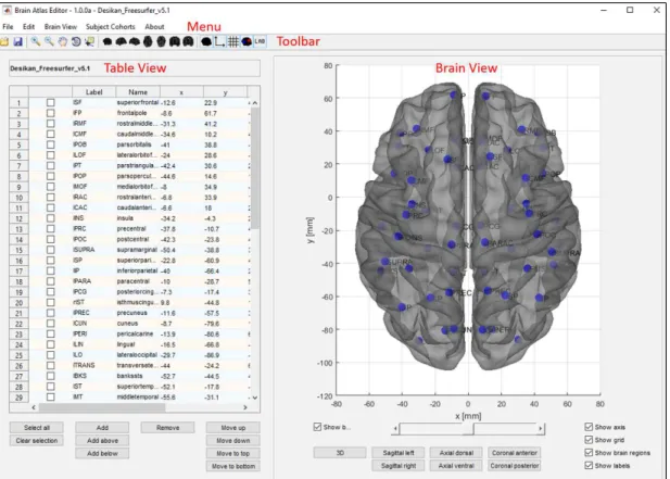
4.5 Screenshot of GUI Brain Atlas . . . 70
4.6 Screenshot of GUI MRI Cohort. . . 71
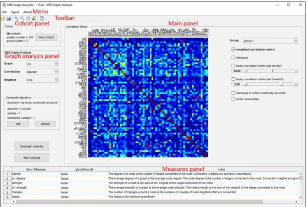
4.7 Screenshot of GUI MRI Graph Analysis. . . 73
4.8 GUI Community structure. . . 74
4.9 Snapshot of GUI MRI Graph Analysis BUD. . . 75
4.10 Interface used to compare the measures of two groups . . . 77
4.11 Structural brain networks in controls, MCI patients, and AD pa-tients. . . 90
4.12 Differences between groups in global structural topology. . . 91
4.13 Differences between groups in nodal structural measures. . . 92
4.14 Functional brain networks and modules in controls and PD-MCI patients. . . 95
4.15 Differences between groups in the nodal functional degree. . . 96
5.1 Brain regions that were used in network construction and analysis. 111 5.2 Structural adjacency matrices. . . 113
5.3 Changes in global network measures as a function of network density.115 5.4 Differences between controls and sMCI, lMCIc, eMCIc, and AD patients in global network measures. . . 116
5.5 Differences between sMCI and lMCIc, eMCIc, and AD patients in global network measures. . . 117
5.6 3. Changes in global network measures as a function of network density. . . 118
5.7 Significant decreases in the nodal clustering coefficient between groups. . . 120
5.8 Significant differences in the nodal closeness centrality between groups. . . 125
5.9 Brain communities in all subject groups. . . 128
6.1 Directed network analysis overview. . . 144
6.2 Changes in global network measures as a function of network den-sity: delays 6-8. . . 151
6.3 Changes in global network measures as a function of network den-sity: delays 9-10. . . 152
LIST OF FIGURES xv
6.4 Changes in global network measures as a function of network
den-sity for longitudinal data. . . 153
6.5 Changes in global efficiency as a function of network density:
de-lays 1-3. . . 155
6.6 Changes in local efficiency as a function of network density: delays
1-3. . . 156
6.7 Changes in clustering coefficient as a function of network density:
delays 1-3. . . 157
6.8 Changes in transitivity as a function of network density: delays 1-3.158
6.9 Changes in modularity as a function of network density: delays 1-3. 159
7.1 Overview of the network reconstruction procedure. . . 166
7.2 Accuracy of network reconstruction. . . 168
7.3 Network reconstruction efficiency of the delayed correlation method.170
7.4 Global network measures as a function of network density . . . 172
7.5 Nodal network measures as a function of density. . . 177
7.6 Community structure in a modular graph. . . 181
7.7 Reconstruction of structural networks derived from DTI data. . . 186
A.1 Changes in global network measures as a function of network den-sity: delays 6-8. . . 227 A.2 Changes in global network measures as a function of network
den-sity: delays 9-10. . . 228 A.3 Changes in global network measures as a function of network
den-sity for longitudinal data. . . 233
A.4 Changes in global efficiency as a function of network density: de-lays 4-6. . . 235 A.5 Changes in local efficiency as a function of network density: delays
4-6. . . 236 A.6 Changes in clustering coefficient as a function of network density:
delays 4-6. . . 237 A.7 Changes in transitivity as a function of network density: delays 4-6.238 A.8 Changes in modularity as a function of network density: delays 4-6. 239
List of Tables
4.1 Characteristics of the structural MRI sample. . . 85
4.2 Characteristics of the fMRI sample. . . 86
4.3 Nodal degree for regions in Module III in PD-MCI subtypes and controls. . . 97
4.4 Nodal degree for regions in Module V in PD-MCI subtypes and controls. . . 98
5.1 Characteristics of the sample. . . 108
5.2 Significant differences in the nodal clustering coefficient between groups. . . 121
5.3 Significant differences in the nodal closeness centrality between groups (FDR - corrected). . . 122
5.4 Summary of the global and nodal network results . . . 126
5.5 Brain communities in all subject groups. . . 129
5.6 Differences in the within-module degree and participation coeffi-cient between groups. . . 134
6.1 Characteristics of Parkinson’s Disease sample. . . 146
6.2 Characteristics of Alzheimer’s sample. . . 147
7.1 Global network measures as a function of network density. . . 174
7.2 Community structure in a modular graph. . . 182
A.1 Differences in global network measures between controls and pa-tients after controlling for scanning site. . . 218
A.2 Correlation between global measures and UPDRS for low resolu-tion networks. . . 229
LIST OF TABLES xvii
A.3 Correlation between global measures and UPDRS for high resolu-tion networks. . . 231
Abbreviations
AD Alzheimer’s Disease
ADNI Alzheimer’s Disease Neuroimaging Initiative
BRAPH BRain Analysis using graPH theory
BUD Binary Undirected Density
BUT Binary Undirected Threshold
CDR Clinical Dementia Rating scale
CDR-SB Clinical Dementia Rating - Sum of Boxes
CTR Controls
DTI Diffusion Tensor Imaging
EEG Electroencephalography
eMCIc early Mild Cognitive Impairment converters
FDR False Discovery Rate
fMRI functional Magnetic Resonance Imaging
G Gyrus
GUI Graphical User Interface
HY stage Hoehn and Yahr stage
Lh Left hemisphere
ABBREVIATIONS xix
MCI Mild Cognitive Impairment
MMSE Mini-Mental State Examination
MoCA Montreal Cognitive Assessment scale
MRI Magnetic Resonance Imaging
PD-CN Parkinson’s Disease Cognitively Normal
PD Parkinson’s Disease
PET Positron Emission Tomography
PD-MCI Parkinson’s Disease with Mild Cognitive Impairment
PPMI Parkinson’s Progression Markers Initiative
Rh Right hemisphere
sMCI stable Mild Cognitive Impairment after 3 years
sMCI-1y stable Mild Cognitive Impairment after 1 year
UPDRS Unified Parkinson’s Disease Rating Scale
UPDRS-III Unified Parkinson’s disease rating scale - Part III
Chapter 1
Introduction
We are surrounded by systems exhibiting complex behaviors that originate from the interactions between few autonomous individuals. Such complex behaviors exist at virtually all scales in nature [1], ranging from the molecular systems [2], the organization of the colonies of bacteria [3, 4], the foraging behavior of ants and bees [5], the organizational patterns of schools of fish [6] or flocks of birds [7] to the collective motion of human crowds [8]. Moreover, many of the man-made systems are also complex, such as the enginnered robotic swarms [9], the internet [10, 11], the power grid [12] or the world wide web [13]. The need for the individual agents to organize in such complex systems arises mainly due to the realization that in many cases, the capabilities of a single individual are not enough to perform a particular task, e.g. to escape from a pray or to find food in the case of the schools of fish, or to support a large amount of electrical energy in the power grid. Therefore, it is necessary for individual elements to work together towards a common goal, which then makes the aim more achievable.
During this cooperative activity each agent would typically have a simple task and would only be aware only of its immediate surroundings without posessing any knowledge of the full picture [14]. For example, in a flock of starlings each bird interacts only with six to seven neighbors [15]; this configuration has been shown to optimize the integrity of the group while at the same time requiring
only minimal action from the individuals [16]. This behavior is also present in man-made systems, for example, in the case of the world wide web, one document would typically have links to only a small number of documents which in turn would link to few others. However, although one document have a small amount of links, the progressive action of reaching new documents at each step ensures that the world wide web is a connected system and every document present on the world wide web is reachable.
The above examples show that studying only a single agent in isolation cannot facilitate full understanding of complex systems. Instead, the interactions be-tween agents are crucial to study the emergent behavior in the complex systems and learn how the actions of the individuals shape their behavior as a whole. One way to accomplish this is to model such systems as networks, a set of nodes, representing the individual agents, and edges, quantifying the interactions be-tween the nodes. Network science has a long history in its application to study complex systems, initially being used in the context of social networks as early as 1940s [17]. Networks continued to be used throught the history in order to study the friendship patterns of people [18] or their business relations [19]. Addition-ally, network studies have been done for citation networks [20] (research papers and citations between them), for world wide web [21] (documents and URLs), for power-grids [12] (generators, transformers and substations, and transmission lines connecting them), airline networks [22] (airports and flights), telephone calls network [23] (phone numbers and telephone calls) or inter-banking networks [24] (banks and claims between banks). In addition to the above mentioned man-made systems, networks are also observed in nature, for example the network of interactions between proteins [25] (proteins and physical contacts between them), the methabolic pathways [26] (biomolecules and chemical reactions) or the food web [27] (species in an ecosystem and their trophic relationships).
Seeing that we have such a diverse set of systems that can be modeled by a single concept, the question arises of whether we are justified to take such approach to the study of complex systems. The answer to this question dates back to 1735 and the Euler’s work to solve the K¨onigsberg bridge puzzle; this is thought to
be the beginning of graph theory, the mathematical framework facilitating the analysis of complex networks. At that time, K¨onigsberg was a captial of Eastern Prussia and was split into four different pieces of land by the river Pregel that passed through the city. Seven bridges were built around the city in order to connect the landmasses, prompting the question of whether one could visit all four landmasses by passing each bridge exactly once [28]. The rigorous proof that such path does not exist was presented by Euler [29]. Crucial to his proof was the realization that the landscape can be represented as a graph; each land becomes a node in this graph and an edge is drawn between two lands connected by a bridge. In this way, he showed that the details of the actual landscape do not need to be taken into account, instead it is only the topological properties of the underlying graph that are essential to solve the problem. This work of Euler is considered to be the first one concerning graphs and provided the basis to the field of graph theory that is at the core of the current methods to analyze complex networks.
Therefore, in a network analysis the real nature of the nodes and edges does not convey any crucial information about the network. The nodes can represent people, molecules, proteins or documents and the edges can represent any physical or abstract connection between them; the crucial realization is that all systems share similar patterns of organization. Therefore, many real networks can be represented by their underlying graph in which all relations are captured by the directions and weights of the edges between the nodes [30]. Then, using the tools of the graph theory this fundamental graph can be studied and various information about its topological structure can be obtained.
Complex networks can be characterized by a vast set of measures that serve to assess various properties of the network [31]. The measures can be nodal and convey information about the individual elements of the network, or they can be global, thus reflecting the properties of the complete network. Most of the measures have been derived for binary undirected networks, i.e. networks that have reciprocal relations and no weight assigned to an edge, for example the sci-ence collaboration network [32]. However, some measures have their counterparts for the case of weighted networks, e.g. network of mobile phone calls [33], and
directed networks, e.g. citation networks [34] (more detailed description of the network distinction based on the nature of the edges and the measures used to characterize such networks is presented in chapter 2). Moreover, on the basis of the type of information they provide about the functioning of the network, mea-sures can be divided as meamea-sures of network segregation, network integration, and influence [31, 35].
Network segregation refers to the localization of the information in a network, indicated by the presence of separate, highly connected sub-networks or patterns of connections [31]. Network segregation can be quantified by the clustering coefficient, defined as the fraction of the neighbors of a given node that are also neighbors to each other; for example, in the context of social networks, clustering reveals how many of one’s friends are also friends with each other. In simplest terms, clustering coefficient counts the fraction of triangles that exist around a node, which conveys information about the network robustness [36, 37]. While clustering is a nodal measure, it can be averaged over all nodes in the network to obtain the global clustering coefficient indicating the extent of segregation in the network. Network segregation can be also revealed by the occurences of motifs, a particular way of connections between a group of nodes that can appear recurrently in a network [38]. Whether some specific sub-network patterns occur in the network more frequently than expected can be studied by comparing the number of motifs of given size in the network of interest to the number of motifs in a random network [39]. In addition to motifs, one can also identify communities in the network. Communities are described as sub-networks that consist of nodes having many more connections with nodes of the same community, when compared to the number of connections with nodes of other communities [40]. Calculating the community structure of a network can reveal an underlying organization or functioning in the network; e.g. in the case of world wide web, different communities might correspond to a set of documents on the same topic [41], or in the context of metabolic networks different communities could be built up from molecules performing similar functions [42].
Measures of network integration evaluate the extent to which nodes in the network can interact and share information between each other. This is most commonly
determined by the concept of shortest distance between two nodes, defined as the lowest number of edges that need to be crossed in order to reach one node from the other. In this context, lower distances between nodes are associated with good integration possibility between the nodes [31]. The shortest path length of a node is calculated as the average of the shortest distances between that node and all other nodes in the graph; lower path length of a node means that the node is well integrated within the network and can easily share information with other network nodes. One can also define the characteristic path length of a network as the average of all nodes’ shortest path lengths. Then, the characteristic path length becomes a measure of the possibility of global interaction within that network. One major drawback of these measures is that paths cannot be meaningfully computed on disconnected networks (the shortest path length of a node is infinity if that node is disconnected). As a result, a new measure, the global efficiency [43], can be calculated for disconnected networks. The global efficiency for a node is calculated as the average of the inverses of the shortest distances between that node and all other nodes in the network, and as such, high global efficiency of a node implies higher degree of integration of that node. The global efficiency of the network is defined as the average of the individual global efficiencies and it has been argued that it could be considered as a better measure than the characteristic path length [44]. Both, the path length and the global efficiency, typically are dimensionless measures and they do not correspond to physical distance.
Just how important a node or an edge is to the structure of the network can be shown by various measures of influence. Most commonly, the importance of a node is expressed through its degree, i.e. the number of neighbors that the node has. The higher degree nodes are considered to be more influential in the network. By making a histogram of the degrees of all nodes in a network, one can obtain the degree distribution in that network; it has been shown that since different networks have different node distributions, networks can be distinguished and categorized based on these distributions [36]. Another measure of influence is the betweeness centrality, which counts how many shortest paths pass through a particular node or edge. This measure can be best interpreted in the context
of information flow. Since a node with high betweeness centrality is likely to be involved in many communication pathways, its removal will cause a disruption of the network and cause a decrease in the network’s efficiency. The variations in the network efficiency can be captured by the measure of vulnerability. Volnerability gauges the changes of the global efficiency of a network when a particular node is removed from the network; thus nodes with high vulnerability are considered to be central to the network [45]. The most important nodes in a network are collectively referred to as hubs. Hubs are integral to the integrity of working efficiency of a network, however, since currently there is no separate measure or a clearly defined way to designate certain nodes as hubs, a combination of the above measures are commonly used for their identification [46].
While the networks’ properties can be very well characterized by calculating some of the described measures, to completely understand the behavior of the real networks it is crucial to understand the origin of such properties and how they affect each other. To this aim, many network models have been developed, each trying to mimic the behavior of real networks as close as possible [47, 48, 49, 50, 51, 52, 53, 54, 55, 56]. The first and simplest model studied was the random graph model, put forward by Erd¨os and R´enyi in 1959 [47]. According to the random model, a network is built by connecting every pair of nodes in the network with a fixed probability p, which can take values between zero and one. Many of the properties of random networks have been mathematically demonstrated and it has been shown that they vary with the value of p. The main result for a random network is that its nodes’ degrees follow Poisson distribution which is quite unlike the real networks which tend to have a power law distribution. The Poisson distribution also does not allow for the existence of hubs (most of the nodes in a random network have comparable degrees), which are very often found in the real networks. Moreover, the random networks do not exhibit a particular community structure, they have low path lengths and low clustering coefficient [57, 58]. Consequently, random networks can very well account for the fact that many nodes in the real networks are reachable by only few connections. However, beyond that, they are very poor model for the behavior of real networks. The main application of random networks is to provide a null model for the evaluation
of a given network property. Namely, if a network’s property is not present in the random model, one can conclude that it cannot be explained by chance and it is an inherent property of that network, requiring an additional explanation [30].
Figure 1.1: Watts–Strogatz model of small-world networks. One starts with a regular network in which all network nodes are placed on a ring lattice. Then, each edge is rewired with fixed probability p. Depending on this probability, one can interpolate between (a) regular network for p = 0 and (d) random network for p = 1. For small intermediate values of p (b, c) one obtains small-world networks. Watts and Strogatz proposed a model (figure 1.1) that was aimed to explain the high clustering and low path lengths present in the real networks [52]. The start-ing point of this model is to create a regular network, in which all network nodes are placed on a ring lattice and connected to their nearest k neighbors. Then, each edge of the network is rewired with a fixed probability p. This rewiring operation involves going through each edge of the network and then moving only one end of that edge to another node in the network chosen at random with prob-ability p. Therefore, for p = 0, the network is a regular network that exhibits high clustering coefficient, but also high path lengths. On the contrary, for p = 1 we obtain a random graph which has short path distances, but also a low clus-tering coefficient. However, Watts and Strogatz showed that between these two extremes, for small positive values of p, one can obtain ”small-world” networks that have high clustering but low path lengths. The reason for this behavior is that the path length drops to low values even for very small p. Even if only few edges are rewired, this creates long-range edges between distant nodes that serve as shortcuts. As a result, as more edges are rewired more shortcuts appear in the network, thereby lowering the path length drastically. On the other hand, the rewiring of an edge from highly clustered community does not have a big effect on
the clustering coefficient. As a result, due to the fact that the path length lowers quicker to its value for the random graph when compared to the clustering coef-ficient, for small non-zero values of p, a network can have both low path length and high clustering [52]. Consequently, the Watts and Strogatz model is very good into predicting the coexistence of small-world behavior and high clustering present in many real networks. However, similar to the random graph model, networks built from this model also have Poisson degree distribution, therefore this model cannot explain the existence of hubs in real networks.
Figure 1.2: Barab´asi–Albert model of growing networks. The starting point of this model is a small network of few nodes (a). Then, a new node with fixed number of connections is added to the network (b). That node makes connections preferentially with the existing nodes that have high degrees (c) and thus becomes a part of the network. By repeatedly performing the preferential attachment mechanism in (b) and (c) the initial network grows in size and the nodes with high degree acquire new connections at much quicker rate than the ones with low degree.
Trying to explain the hubs and the power law degree distribution observed in real networks, Barab´asi and Albert [30, 56], inspired from the structure of the world wide web, proposed a model of growing networks (figure 1.2). Their model is based on the growth of a network by adding nodes that attach preferentially to the existing nodes with higher degrees. More specifically, the model starts with a small network. Then, at each step a new node is added to the network by making fixed number of connections with the existing nodes in the network. The probability of making a connection with a node is proportional to that of node’s degree in the network. Therefore, this model results in a network exhibiting the rich gets richer phenomenon, thereby favoring the nodes with high degrees that
have been present in the network early on. The networks resulting from this model are scale-free networks having a degree distribution following a power law with an exponent of three. This model is considered to be an important one when describing the real networks which also follow power law degree distribution, e.g. the internet or world wide web [59]. In an attempt to make this model more realistic, e.g. to obtain a flexible exponent in the power law or to improve the clustering behavior, many alterations to the original model were proposed in the literature, for example nonlinear preferential attachment [60].
The brain is one of the most complex systems, built up from approximately 1011
neurons connected by 1014 synapses organized in a three dimensional space by
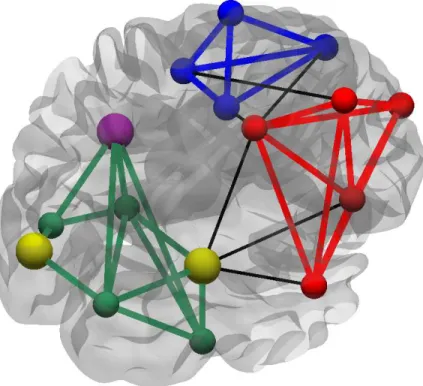
optimizing the wiring cost to get maximum flexibility [61]. The neurons are connected by a convoluted net of connections acting as a scaffold supporting the emerging complex dynamic patterns that are considered to shape cognition [62, 63]. While each nerve cell has a particular role to play in this behavior, cognition and other brain functions can only be observed when many neurons are linked together in small networks, subsequently combining to form larger and larger networks eventually building the whole nervous system, as illustrated in figure 1.3. Therefore, to gain insight into the brain functions, we would need to study the brain’s complex networks at many levels, from small neuronal circuits to large-scale brain networks, in addition to studying the complex dynamic patterns that emerge from their collective behavior [64].
Figure 1.3: From a single neuron to brain. A neuron is the fundamental building block of the brain which can receive and process information. In order to pass information between each other, neurons combine through electrical and chem-ical synapses to form a network. Many neuronal networks combine into larger ones eventually forming the brain; all brain functions arise due to the collective behavior of this large number of neurons. Adapted from [65, 66, 67]
Representing the brain as a complex network and analyzing its underlying organi-zation could reveal some information about the brain functioning. For example, the brain is made up of spatially distributed areas that have highly specified functions but are still able to communicate efficiently between each other. This illustrates the two basic organizational principles in the brain, functional segrega-tion and funcsegrega-tional integrasegrega-tion, and they both can be characterized by calculat-ing the appropriate measures on the brain networks as discussed above [68, 31]. Moreover, it has been shown that there is a lot of characteristic activity in the human brain even when the person is at rest [69, 70]. This dynamic activity during rest is supported by the underlying physical network of neurons; there-fore investigating how the structural architecture shapes the resulting dynamic behavior could provide great insight into why such networks appear even at rest [64]. Finally, many neurodegenerative diseases or brain traumas can be related to a corresponding damage in the structural connectivity in the brain [71, 72]. Therefore, the quantification of some abnormal topological properties of brain networks present in patients when compared with healthy individuals, could be used as diagnostic markers in some diseases. In addition to the above examples, brain networks could be used to provide insight, for example, into the dynamic patterns that result from an external stimuli to the brain, and into the change of cognition abilities over time [64].
In the early beginings of the neuroscience, the visual inspection of the anatomy of the brain by using techniques, like staining and sectioning the brain tissue, were the common way to obtain information about the brain’s composition [73]. In fact, most of the early knowledge about the working principles of the neurons came by measuring electrophysiological recordings of single intact neurons. While such recordings do allow for direct measurements of the electrical properties of the neuron with high spatial and temporal resolution, the need for the intact brain tissue means that they are highly invasive techniques and could not be applied directly to humans [64]. In order to extract information about the human brain, there was a necessity for a non-invasive imaging technique that could produce large sets of data that could be subsequently analyzed. Electroencephalography (EEG) and magnetoencephalography (MEG) are the first such techniques to be
applied. They measure the fluctuations that occur due to neuronal currents by placing a series of sensors near the scalp. While they have high temporal resolu-tion, they do not have good spatial resolution because they record electromagnetic potentials resulting from the collective currents of large populations of neurons. In addition, the reconstruction process to obtain the real sources responsible for these signals is ambiguous and depends highly on the statistical technique used to process the data [74]. Another frequently used noninvasive technique that helped in the expansion of the neuroscience research is functional magnetic resonance imaging (fMRI). Using the contrast derived from the differences in magnetic sus-ceptibility of oxygenated and deoxygenated blood (shortly termed BOLD contrast where BOLD stands for ”Blood Oxygenation Level Dependent”) fMRI can mea-sure metabolic activity in the brain. Thus, fMRI does not meamea-sure the electric currents (or neuronal activity) directly, rather it measures the changes that this activity causes in the blood flow and oxygenation [75]. The fMRI imaging has high spatial resolution (usually of the order of submillimeters in humans [76]) with temporal resolution of the order of seconds, which is partially due to the delayed response of the BOLD signal from the onset of the neural activity [77]. The main aim of the imaging techniques described above (fMRI and EEG) is to directly measure or infer the neuronal activity ongoing in the brain. In addition, there are few noninvasive techniques that are designed to characterize the struc-tural connections between the neural cells. One of the most widely used technique is the Diffusion Tensor Imaging (DTI), in which the image contrast is obtained by using the anisotropic diffusion of water molecules inside the neural tissue. In particular, the macroscopic axons provide a strong orientational confinement for the water molecules; the easiest direction in which they can diffuse is the direction of the axon. One can reproduce the direction of preferential diffusion of the water molecules in each voxel by using a tensor model [78]. Commonly, a tractography is performed on these images in order to completely reconstruct the white matter paths followed by the diffused molecules of water [79].
Another technique to measure the structural connections is structural MRI, which can generate images that can differenciate between white and gray matter in the brain due to their different compositions. Using certain morphometric techniques
[80], the cortex can be parceled and one can calculate a measure of interest for each region, for example the thickness of the cerebral cortex. Thus, the connectivity between any two regions is estimated indirectly; the strength of their connection is given by the Pearson’s correlation coefficient of the cortical thickness values for both regions, across a group of subjects. In contrast to the DTI imaging, by using the structural MRI method one cannot estimate the structural connections for a single subject.
Although there exist various imaging techniques, the building of complex net-works from empirical data obtained from these techniques proceeds among few common steps [71]. The first step includes identification of the nodes of the network. The nodes in brain networks represent brain regions and they can be defined by some anatomical atlases in structural and functional MRI or by the position of the electrodes in EEG. This step is followed by the definition of the edges in the network. Each edge describes the degree of interaction between the two nodes it connects. Depending on the neuroimaging technique, edges can be derived in different ways. For example, in structural MRI edges are typically correlations between the cortical thickness values, however in functional MRI the edges are correlations between time series. After calculating the edge stengths for each pair of nodes in the network, these estimates are compiled into an adjecency matrix. Finally, some graph measures are calculated to characterize the network and their statistical significance is reported by comparing them to the measures derived from a set of random networks. It should be noted that each of this steps is essential in the analysis but there is not a unique way to execute them, i.e. some decisions are required at each step, for example one needs to choose a par-ticular parcellation scheme for the brain. Therefore, each decision will influence the results obtained from this analysis; two brain networks can be meaningfully compared only if they have been derived from the same procedure [71].
The existence of many different neuroimaging techniques to capture different aspects of brain connectivity coupled with the plethora of computational methods to analyze the data, results in different ways to describe the networks in the brain. The first method is to build structural networks, defined as the physical web of connections between the different neurons. Then, we could also build
functional networks in the brain which describe the dynamic interactions, or functional correlations, of the neurons. Finally, effective connectivity, or the causal interactions between different neuronal elements, could be also examined. Structural connectivity refers to the complex web of anatomical connections that link distinctive neuronal elements in the brain, termed as the connectome [81]. These structural connections exist in the brain on multiple scales, from networks of few neurons connected by synapses to brain regions connected by axonal pro-jections. These networks are most frequently derived from DTI and structural MRI and they represent topological association patterns. However, it has been shown that there is a relation between the topological and physical distances in structural networks; the neurons in the proximity of each other have higher prob-ability to be connected [71, 82]. Moreover, the structural networks are thought to be susceptible to change only on longer time scales (e.g. days) while remaining relatively stable on shorter time scales of the order of minutes [35].
Functional connectivity is defined as the statistical correlations between activity patterns produced from spatially distinctive neuronal populations [83, 84]. Func-tional connectivity data is extracted from funcFunc-tional MRI, EEG and MEG in the form of time series data. The pairwise coupling strengths are estimated by calculating a certain measure between the corresponding time series, such as cor-relation, coherence or mutual information [85]. As correlation does not necessary imply causation, functional networks do not convey information about the causal relation between its elements. Moreover, differently from structural networks, functional connectivity is very time dependent and also highly dependent on any external sensory input [35].
Effective connectivity aims to describe networks that reflect the influences that one neural system has on another [83, 84]. Effective connectivity is also time dependent and often it is inferred by modulating the neuronal activity by external stimuli or specific tasks. The effective networks are commonly derived by applying a particular model to the time series obtained from different neural elements, therefore the validity of the particular effective network depends highly on the validity of the modeling procedure [83]. One of the most commonly applied model
is the Granger causality [86, 87], which is based on the idea that in the interactions between two events, the cause will always occur earlier in time than the effect. For example, consider the direct causal relation between two regions, from A to B. The Granger causality assumes that in such case, events in A must always precede events in B. Moreover, this method quantifies how much information one has in order to make a prediction about the future values of B, by considering the past values of A. Therefore, Granger causality is fully based on the statistical behavior of the observed time series and does not make any explicit assumption about the structural connections between the neural elements. On the other hand, models such as Dynamic Causal Modeling (DCM) [88] and Structural Equation Modeling (SEM) [89] need a priori postulation of structural networks in order to infer the effective connectivity. As a result, they are not able to test many possible network arrangements; moreover DCM is designed only in the framework of task-related experiments since it requires the timings of the external stimuli as input.
What can these different connectivity types reveal about the organization of the brain? Small-world organization in the structural networks of the brain was re-ported by many studies using various imaging techniques, including correlation of cortical thickness in structural MRI [90] and diffusion weigthted MRI [91]. The small-world organization manifests itself in the high clustering coefficients and low path lengths in these networks. These properties support the notion that the brain is organized in order to balance the anatomical and functional segregation (described by the high clustering coefficient as discussed above) with their inte-gration on the global scale (manifested by the low path length). Furthermore, it was realized that the structural brain networks can be very well separated into distinct communities, thus explaining the origin of the high clustering coefficient [35]. The communities were found to consist of elements that have similar physi-ological responses, have more connections with elements of the same community and, in general, the structural communities form compact functional systems [92, 93]. The existence of separate communities with many densely connected elements is useful for the support of the functional segregation, by providing many connections for efficient communication of the specialized brain regions on
one hand, while restricting the information flow during the whole network by providing boundaries between these specialized regions on the other. Further-more, it was shown that the communities communicate between them by making use of hubs [46], nodes that have very high degrees and betweeness centrality. Moreover, hubs are densely interconnected with each other [94] forming rich club organization that is mainly used to facilitate the information flow in the network [95, 96, 97].
Small-world properties have also been identified in functional networks with dif-ferent measures estimating the functional connections [98, 99] and they have reported a power law degree distribution that is exponentially bounded [99]. It has also been shown that the functional networks exhibit significant modularity that can be used to explain their small-worldness [100] analogously to structural network studies. PET has been used to define the default functional network of the human brain at rest [101] and it has been shown the dynamics of a resting brain can be broken down into a small set of “resting-state networks” [35]. By studying complex networks in the brains of individuals with some neurodegen-erative diseases and identifying the aberrations in their topological organizations one can obtain many insights about the particular disease [102]. This is possible because it has been postulated that the impairments in cognition that result from the disease occur due to the impact that the disease has on the arrangement of brain connectivity [103]. For example, it has been shown that the structural net-works in patients with schizophrenia [104] have abnormal organization manifested by the increased connection distance and the loss of the hierarchical organization. Alterations of the small-world topology of the structural networks, measured as increased clustering and path lengths, were also detected in Alzheimer’s disease (AD) [105]; such findings were also reported for the corresponding functional networks derived from EEG [106]. Similar results were obtained from fMRI and MEG studies for AD [71], autism, epilepsy, multiple sclerosis, Parkinson’s disease [96, 97, 102]. Nonetheless, it should also be noted that while most studies present compelling evidence that neural disorders result in abnormal network organiza-tion in patients, a disparity between some results still remains. Therefore, such results need to be considered with caution as the particular findings may depend
on the clinical heterogeneity of the patient and control group as well as on the particular imaging and data analysis methods that were being used [71].
Although networks derived from different imaging modalities can reveal many im-portant properties of the brain organization as outlined above, to get full under-standing of the operation of the brain one needs to consider the relation between the structural architecture and the dynamic patterns that it promotes. There are many studies, derived from experimental observation or theoretical models, that strongly support the notion that physical links in the brain can shape neu-ronal dynamics [107]. In particular, having the information that the structural network has a small-world organization, one could infer that the expected func-tional connectivity would be manifested by many short-range interactions and smaller number of long-range interactions [63]. The relation between structure and function can be examined on many scales, for example by simulating neural circuits on the microscale or brain regions in the large scale brain networks. The most common method to asses this relation is to use a model that infers the func-tional connectivity from a structural substrate, and then matches the simulated dynamics with the empirically measured one [107]. Although this procedure will heavily depend on the computation models used to produce simulated functional data as well as the measures used to estimate the connection strengths in the empirical functional data, many studies converge to the conclusion that structure does shape function [107], however the inference of structural connectivity from functional data is less straightforward [108].
In this thesis, I will show that directed networks constructed in the brains of Alzheimer’s and Parkison’s patients are more sensitive to the disease when com-pared to their undirected analogues. Moreover, I establish that the functional networks built by the standard correlation methods do not faithfully represent the underlying structural architecture. Instead, I will demonstrate, by using nu-merical simulations, that the underlying structure invariably introduces delays in the dynamic behavior of neurons and propose the delayed correlation method that utilizes these delays to identify up to 70% of the connections in the cor-responding structural network. In order to carry out these analyses, we have
developed BRAPH–BRain Analysis using graPH theory, an object oriented Mat-lab software that can be used to perform connectivity analysis of brain networks derived by various imaging modalities. My thesis can be divided into two parts, background and application of graph theory to brain connectivity. In the first part, I will introduce the basic concepts of graph theory and the most commonly used measures to characterize the graphs (chapter 2). Then, in chapter 3, I will describe how to build the brain networks from data obtained by some common imaging modalities, before I present BRAPH and its functionalities in chapter 4. The second part of my thesis is concerned with the application of graph theory in brain connectivity studies. In particular, I will discuss the changes in the topo-logical properties of undirected and directed brain networks (chapters 5 and 6 respectively) in Alzheimer’s and Parkinson’s patients, before demonstrating how temporal delays in the neuronal dynamics can help us to reconstruct neurons’ structural connections in chapter 7.
Chapter 2
Graph Theory Concepts
In the 1970s K¨onigsberg was a captial of Eastern Prussia and a very important trading center. The city was built on the top of the river Pregel and the two banks of the river separated the city into four different pieces of land. In time, seven bridges were built around the city in order to connect the different landsmasses, the resulting landscape had the look as shown in figure 2.1(a). This proved to be the start of a puzzle, with people wondering whether it was possible to visit all four landmasses by crossing every bridge exactly once. There were many attempts to find a solution by drawing all possible ways to cross the seven bridges, however a correct path could not be found [28].
The first rigorous proof that such path does not exist was provided by Euler [29]. He was able to show this by representing the whole landscape as a graph (figure 2.1(b)) in which each landmass is represented by a node and an edge is drawn between two nodes only if the corresponding landmasses are connected by a bridge. By inspecting the resulting graph, he was able to make the observation that if a path connecting all landmasses without passing twice by the same bridge exists, the only nodes with odd number of edges must be the ones corresponding to the starting and ending point of the path. If a node in the middle of the path has an odd number of connections 2n + 1, then 2n connections will be used to arrive to and leave from the node, therefore one connection will always be left
Figure 2.1: K¨onigsberg’s bridges and the corresponding graph. (a) The two banks of the river Pregel (drawn in blue) split K¨onigsberg into four different pieces of land that were connected by seven bridges (shown in red). (b) The corresponding graph of the city in which each landmass is represented by a node and connections between the landmasses are drawn if there is a bridge connecting them. Adapted from [109].
unused [30]. Since in the graph in figure 2.1(b) all four nodes have an odd number of connections, it leads to the conclusion that the required path cannot be found. Euler’s work was important because he showed that in order to study a complex system, we do not require a complete knowledge of the properties of the system, for example the size of the landmasses or the length and curvature of the bridges. Instead, we could represent the complex system as a graph and we could gain all the relevant information about the system by studying only the topological properties of that graph.
In this chapter, I will give an overview of the measures that are most commonly used to characterize the properties of a graph. I first give a brief introduction to graphs and how they can be represented; then I discuss the different types of graphs that emerge from the different nature of their edges. Finally I present the definitions of some graph measures and explain the various techniques and algorithms that can be used to calculate them.
2.1
Graphs
A graph is composed of a collection of nodes that are linked by edges. An example of a sample graph is shown in figure 2.2(a) where each circle represents a node
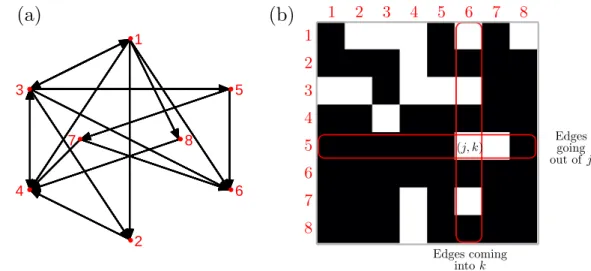
and each line represents an edge. This illustration of a graph is very intuitive but it can become very tangled and convoluted as we increase the number of nodes and edges. 1 2 3 4 5 6 7 8 1 2 3 4 5 6 7 8 1 2 3 4 5 6 7 8 (j, k) Edgesgoing out of j Edges coming into k
(a)
(b)
Figure 2.2: A simple graph and connectivity matrix. (a) An example of simple binary graph and (b) the adjacency matrix that corresponds to this graph. Figure 2.2(b) shows that a graph can be instead described by compiling all nodes and edges in a matrix, called adjacency matrix. Each element of the matrix represents an edge between the corresponding nodes; for example, in figure 2.2(b), the element (j, k) represents the edge that goes from node j to node k. The rows of the adjacency matrix are regarded as edges that are going outwards from a node; for example, row j represents the edges that are going out from node j. On the contrary, each column depicts the edges that arrive inwards to a node; for example, all entries in column k show the edges that are arriving to the node k. The representation of graphs as adjacency matrices is appealing because this allows one to utilize highly-optimized algorithms that are based on linear algebra [110]. Moreover, it should be noted that the particular way in which nodes are ordered in the adjacency matrix does not affect the evaluation of the graph measures, but it only influences the graphical representation of the adjacency matrix.
2.2
Types of graphs
Each edge in a graph can be associated with a weight and direction, based on these characteristics of the edges, four types of graphs can be identified (figure 2.3):
Weighted directed (WD) graphs. A real number that quantifies the
strength of a connection is associated with each edge. The edges represent direct connections, i.e. a given node j can have a connection to node k without the need for the node k to be connected with node j).
Weighted undirected (WU) graphs. A real number that quantifies the
strength of a connection is associated with each edge. The edges represent undirect connections, i.e. if a given node j has a connection to node k, then node k is also connected to node j. For these graphs, the adjacency matrix is symmetric.
Binary directed (BD) graphs. The edges represent directed connections
and can take values of 0 (in which case they represent the absence of a connection) or 1 (they represent the existence of a connection). In this type of graphs the strength of a connection is not quantified.
Binary undirected (BU) graphs. The edges represent undirected
con-nections and can take values of 0 (the absence of a connection) or 1 (the existence of a connection). In this type of graphs the strength of a connec-tion is not quantified. Moreover, the adjacency matrix is symmetric.
Figure 2.3 shows that these four types of graphs are directly linked to each other, and a transformation between each graph type can be done in the following ways:
Weighted to binary. A weighted graph can be transformed into a binary
one by the process of thresholding. This process entails the specification of a threshold value and assigning a value of 1 to the edges that have strengths above this threshold and 0 to those edges that have strengths below the
1 2 3 4 5 1 2 3 4 5 1 2 3 4 5 1 2 3 4 5 1 2 3 4 5 1 2 3 4 5 1 2 3 4 5 1 2 3 4 5 1 2 3 4 5 1 2 3 4 5 1 2 3 4 5 1 2 3 4 5
Weighted Directed Weighted Undirected
Binary Directed Binary Undirected Symmetrize
Symmetrize
Binarize Binarize
Figure 2.3: Graph types. Based on the nature of their edges, the graph can be classified as weighted or binary (according to the weights of the edges) or as di-rected or undidi-rected (based of the directionality of the edges). By eliminating the information about the edges’ directionality (i.e. symmetrization) one can convert a directed graph into an undirect one. Similarly, by removing the information about the edges’ weights (i.e. thresholding) a weighted graph can be converted into a binary graph.
threshold. The threshold value can be identified a priori, or alternatively it can be determined as to ensure that the resulting graph has a certain density, i.e. the fraction of edges that are connected. The choice of the threshold is relevant in the comparison of binarized graphs, because such comparison is only meaningful when the two graphs are compared at fixed threshold or at fixed density.
undirected one by the process of symmetrization, which removes the infor-mation about the directions of the edges. This is accomplished by sym-metrizing the adjacency matrix of the graph. Symmetrization can be per-formed along several possible directions, e.g.:
1. Sum. The adjacency matrix and its transpose are added to each other. 2. Average. Average of the adjacency matrix and its transpose.
3. Minimum. The adjacency matrix is compared to its transpose; for each element the smaller value of the two is used.
4. Maximum. The adjacency matrix is compared to its transpose; for each element the larger value of the two is used.
2.3
Graph measures
Two general categories can be used in order to classify the graph measures:
1. global measures refer to the properties of a graph as a whole, and therefore, the information they convey is captured by a single number for each graph; 2. nodal measures refer to the properties of each node in a graph, and there-fore, they consist of a vector of numbers — one for each node of the graph.
In this section I will briefly discuss the most common graph measures. Most of the measures have been derived for binary and undirected graphs, however some of them have extensions or analogues for weighted or directed graphs. Therefore, for each measure, I will indicate to which kind of graph it belongs by denoting W (= weighted graphs) or B (= binary graphs), and D (= directed graphs) or U (= undirected graphs). If no particular letter is assigned to the measure, it means that the measure can be used in both cases.
2.3.1
Degree
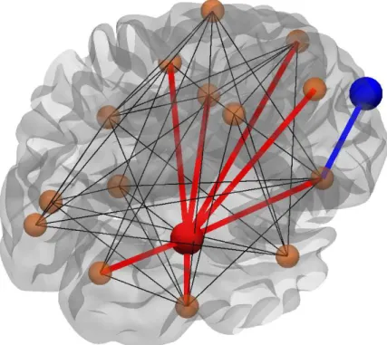
Degree (nodal, BU) is defined as the total number of edges that are connected to a node. The average degree (global, BU) can be calculated as the average of the degrees of all nodes.
Figure 2.4: Degree of a node. The red is an example of a high degree node(i.e. it has a high number of neighbors), while the blue node possesses a low degree (i.e. it has a small number of neighbors).
In-degree (nodal, D) is defined as the total number of edges that are going inwards to a node. Its global extension is the average in-degree which is the average of the all nodes’ in-degrees.
Out-degree (nodal, D) is defined as the total number of outward edges that originate from a node. Its global extension is the average out-degree defined as the average of all nodes’ out-degrees.
number of edges across the rows or columns of the adjacency matrix. Since the adjacency matrix is symmetric for BU graphs, both calculations will yield the same result; in other words, for BU graphs, the in-degree and out-degree are equal. For BD graphs, a sum over the columns of the adjacency matrix gives the in-degree, while the out-degree is calculated as sum over the rows. In these graphs, the degree is the sum of in-degree and out-degree. For W graphs, the weights need to be ignored when the degree is calculated. Due to this reason, one needs to first binarize the adjacency matrix so that every edge that corresponds to non-zero weight is set to 1, while the rest remain as 0. Then, the degrees can be calculated on this binarized adjacency matrix analogous to the calculation for B graphs.
A property of a graph closely related to the degree is the degree distribution,
denoted by pK, which represents the probability that a node chosen at random
has degree K. The degree distribution can be calculated as the histogram of the degrees of all nodes in the graph, normalized to 1.
2.3.2
Strength
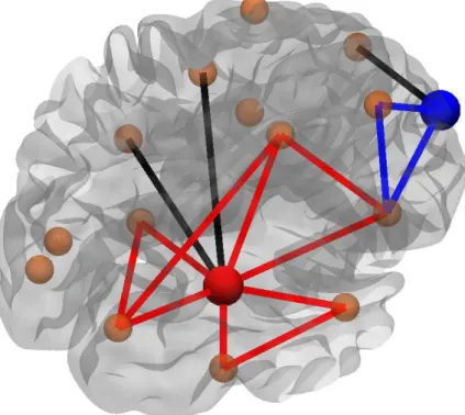
Strength (nodal, WU) is defined as the sum of the weights of all edges connected to a node [111]. The average strength (global, WU) can be calculated as the average of the strengths of all nodes.
In-strength (nodal, WD) is defined as the sum of the weights of all edges that are going inwards to a node. Its global extension is the average in-strength which is the average of the all nodes’ in-strengths.
Out-strength (nodal, WD) is defined as the sum of the weights of all outward edges that originate from a node. Its global extension is the average out-strength defined as the average of all nodes’ out-out-strengths.
Methodological notes: For WU graphs, the sum over either rows or columns of the weighted adjacency matrix gives the strength of each node. For WD graphs,
Figure 2.5: Strength of a node. Even though the red node has a low degree, it possesses a higher strength (there is only one connection that has a very high strength of 0.9), while the blue node has a higher degree but smaller strength (although it has 7 connections, each has low strength of only 0.1).
out-strengths are calculated as sums over rows, in-strengths are calculated as sums over columns; the strengths are defined as the sum of the in-strengths and out-strengths.
2.3.3
Eccentricity
Eccentricity (nodal) is defined as the maximal distance between a given node and any other node in the graph [112]. The global version is the average eccen-tricity that can be calculated as the average of the eccentricities of all nodes. In-eccentricity (nodal, D) can be calculated as the maximum of the incoming distances from all other nodes to a given node. Its global extension is the average
in-eccentricity which is the average of the all nodes’ in-eccentricities.
Out-eccentricity (nodal, D) can be calculated as the maximum of the outgoing distances from a given node to all other nodes. Its global extension is the average out-eccentricity which is the average of the all nodes’ out-eccentricities. Two other global measures can be specified once we know all nodes’ eccentricities. The first one is the radius of the graph which is defined as the minimum eccen-tricity of all nodes. One can also define the diameter of a graph and calculate it as the maximum eccentricity of all nodes.
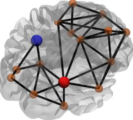
Figure 2.6: Distance between nodes. While there exist many paths between the two green nodes (e.g. the red and blue paths), the distance between the two is defined as the shortest possible path between them (the red path).
Methodological notes: For every graph, one can calculate a distance matrix; the elements of this matrix are the distances (the shortest path lengths) between all pairs of nodes in the graph. Then, the eccentricity of a given node is taken to be the maximum of all the distances that are calculated for this node. For D