η -* ■ ‘ •^• ;: ϊί,’^ ч . ‘'■‘ .ί i ' f ·* . \^·*'· Л >·^·* л “ ·'!. ,Л>. ■· * ■ /'ji «·ΐ.ι,ϊ 5 э а S ^ 5
/393
THE FISHER HYPOTHESIS: A MULTI-COUNTRY
ANALYSIS
A THESIS
SUBMITTED TO THE DEPARTMENT OF ECONOMICS AND THE INSTITUTE OF ECONOMICS AND SOCIAL SCIENCES
OF BILKENT UNIVERSITY
IN PARTIAL FULFILLMENT OF THE REQUIREMENTS FOR THE DEGREE OF
MASTER OF ARTS
By
M oham ed Mehdi Jelassi August, 1999
3
с
НБ 5S0
•J4S
I certify that I have read this thesis and that in my opinion it is fully adequate, in scope and in quality, as a thesis for the degree of Master of Arts.
Assist. Prof. Hakan Berument(Principal Advisor)
I certify that I have read this thesis and that in my opinion it is fully adequate, in scope and in quality, as a thesis for the degree of Master of Arts.
I certify that I have read this thesis and that iiyn y opinion it is fully cvdeqiuite, in scope and in quality, as a thesis fqrjA:6aegree of Master of Arts.
Prof. Mehmet Caner
Approved for the Institute of Economics and Social Sciences:
ABSTRACT
T H E F IS H E R H Y P O T H E S IS : A M U L T I-C O U N T R Y A N A L Y S IS
M oham ed Mehdi Jelassi M .A . in Economics
Supervisor: Assist. Prof. Hakan Berument August, 1999
There is a long tradition of testing the Fisher hypothesis on the long run relationship between inflation and nominal interest rates. In this study, we examine the before tax strong version of the Fisher hypothesis for a sample of countries, in an attempt to extend the available literature. Using an error correction modeling approach suggested by Moazzarni [30] which cillows for direct estimates of the long run coefflcients, we show that the strong version of the Fisher hypothesis tends to hold for more than half of the countries under study. In addition to that we point to the fact that under complete financial deregulation, there is a higher chance for the Fisher hypothesis to hold in line with the suggestion of Olekalns [33].
Key words: Fisher hypothesis; Inflation; Interest rate.
ÖZET
F IS H E R H İP O T E Z İ: Ü L K E L E R İN B İR A N A L İZ İ
M oham ed Mehdi Jelassi iktisat Yüksek Lisans
Tez Yöneticisi: Assist. Prof. Hakan Berument Ağustos, 1999
Enflcisyon ve nominal faiz oranlan arasındaki ilişkiyi Fisher Hipotezi ile test etme konusunda uzun zamandır süregelen bir gelenk mevcuttur. Bu çalışmada, Fisher Hipotezinin vergi öncesi versiyonunu, mevcut olan literatürü genişletmek amacıyla değişik ülke gruplarına uyguluyoruz. Bu amaçla Moazzarni [30] tarafından önerilmiş olan ve uzun vadeli katsayıları hata düzeltme modelini kullarnasına izin veren modelini incelenmiş ülkelerin yarısından çoğu için uygun olduğunu gösteriyoruz. Buna ilaveten Olekalns [33] tarafından da önerildiği gibi komple bir finansal deregülasyonda Fisher Hipotezinin gerçekleşme şansının daha yüksek olduğunu tastikliyoruz.
Anahtar sözcükler: Fisher hipotezi, Enflasyon, Faiz oranı
ACKNOWLEDGEMENT
Special thanks to Prof. Hakan Berument for supervising this work. I am also greatful to Prof. Syed Mahmud, for his availabilty and help on anything I asked for, and Prof. Serdar Sayan who have been supervizing me with patience cincl everlasting interest and being helpful in any way during my graduate studies.
Contents
1 In tr o d u c tio n1
1.1 in trod u ction ... 1 2 L itera tu re R e v ie w 5 2.1 Literature R e v ie w ... .5 3 T h e B asic M o d e l 11 3.1 The Basic M o d e l ... 114 E s tim a tio n and R esu lts 15
4.1 Estimation and R esu lts... L5
4.1.1 D a t a ... L5
4.1.2 Estimation Issues and the R e su lts... 17
4.1.3 Robustness A n a ly s is ... 27
CONTENTS 5 C o n clu sio n 5.1 Conclusion Vlll 39 39
List of Tables
4.1 The list of the countries s t u d ie d ... 16
4.2 Long-term Effect of Inflationary Expectations on the Nominal Interest Rate: Developed C o u n trie s ... 19
4..3 Long-term Effect of Inflationary Expectations on the Nominal Interest Rate: Developed Countries continued 20
4.4 Long-term Effect of Inflationary Expectations on the Nominal Interest Rate: Developing C ountries... 21
4.5 Long-term Effect of Inflationary Expectations on the Nominal Interest Rate: Developing Countries continued... 22
4.6 Long-term Effect of Inflationary Expectations on the Nominal Interest Rate: Developing Countries continued... 2.3
4.7 The Q-statistics: F-values for the developed co u n trie s... 27
4.8 The Q-statistics: F-values for the developing countries 28
4.9 The ARCH-LM test: F-values for the developed countries . . . . 29
4.10 The ARCH-LM test; F-values for the developing countries . . . 30
4.11 The Chow Breakpoint Test: F-statistics, Probabilities for the developed cou n tries... 33
4.12 The Chow Breakpoint Test: F-statistics, Probabilities for the developed countries con tin u ed... 34
4.13 The Chow Breakpoint Test: F-statistics, Probabilities for the developing countries 35
4.14 Robustness Analysis for the US adjusted m o d e ls ... 37
4.15 The adjusted models for the US d a t a ... 38
Chapter 1
Introduction
1.1
Introduction
The effect of inflation expectations on nominal interest rates, emphasized by Thornton (1802), and later embodied by Fisher (1930) [8] in the ’’ Fisher hypothesis” , arguing that in its strong form, the nominal interest rates rise point-for-point with expected inflation, leaving the real interest rate unaffected, is one important macroeconomic relationship of neoclassical monetary theory.
The P'isher effect states that, in the long-run equilibrium, a change in the rate of growth of the money supply leads to a fully perceived change in inflation and a concurrent adjustment of nominal interest rates. Implicit in this assumption is that in the long-run, real interest rates will not respond to movements in expected inflation, rather, changes in inflation will be cibsorbed in nominal interest rates, leaving real interest rates constant, ceteris paribus.
constant over time, but that changes in them will be the result of changes in real economic factors. If there is evidence that real interest rates move in response to expected inflation, then inflationary movements have not been totally absorbed in nominal interest rates and the Fisher hypothesis does not hold.
CHAPTER 1. INTRODUCTION 2
Fisher’s premise is that the real rate of interest on a financial asset is constant over time and therefore a fully perceived change in the rate of inflation is accompanied by a one-to-one change in the nominal rate of interest. In other words, the strong version of the Fisher effect states that the nominal interest rate fully incorporate anticipated changes in the price level. However, this hypothesis requires assumptions regarding the absence of taxation, and zero interest elasticity of money demand.
The argument that full adjustment of the nominal interest rate requires a perfectly inelastic money demand function dates back to Sargent [36], and may be earlier. In fact, Sargent showed that, in the context of a dynamic Keynesian income-expenditui’e model that the instantaneous effect of a rise in expected inflation is to increase the demand for investment as the real interest rate falls. Should the LM curve have a positive slope, the nominal interest rate rises, initially, by less than the increase in anticipated inflation. Over time, however, complete adjustment is achieved. In contrast, a vertical LM curve means that the nominal interest rate adjusts instantaneously. However, Visco [40] showed that even a vertical LM curve does not guarantee complete adjustment. Other arguments supporting partial adjustment have been forwarded by Mundell [32], Fried and Howitt [9].
CHAPTER 1. INTRODUCTION
of money demand, opens the way to a variety of interest rate responses to anticipated inflation.
For example, taxation implies that the nominal rate should include a premium over and above the anticipated rate of inflation. On the other hand, an interest-elastic money derncind function implies partial adjustment [.36]. Once allowance is made for these factors, the Fisher effect is more realistically interpreted to mean the existence of a positive relation between anticipated inflation and the nominal rate of interest. Whether this involves partial, complete or over adjustment can be inferred from the data.
There is a long tradition of testing the Fisher hypothesis. Our main intention in this work is to test the Fisher hypothesis across countries using the method suggested by Moazzami [30]. In Moazzami [30], the Fisher hypothesis is modeled within a framework that allows direct estimate of the long run coefficients, while taking into consideration the short run dynamics.
Performing this analysis provides us with several insights concerning the Fisher hypothesis. It allows us to measure to what extent does the long run Fisher effect holds. In other words, does the long run Fisher effect holds for all types of economy, or does it hold for only some economies? In addition to that does it hold strongly or partially?
Besides this, we have performed our empirical work on developed and developing countries, in hopes of detecting any differences concerning the conditions under which the Fisher hypothesis tends to hold. In addition to that, we tried to extend the literature on the Fisher hypothesis by examining a sample of developing countries, since little is reported for testing the Fisher hypothesis in such countries.
CHAPTER 1. INTRODUCTION
In chapter 2, we revise the existing literature on the Fisher hypothesis, by mainly presenting the methodologies used and the results reached. In chapter 3, we present the basic model, suggested by Moazzami [30], that we have employed to carry out our study. In chapter 4, we provide our results, by presenting the estimated models, and the robustness analysis performed to validcite these models. Finally, in chapter 5, we summarize our findings.
Chapter 2
Literature Review
2.1
Literature Review
There is a long tradition of testing the Fisher hypothesis, that the nominal rate of interest incorporates anticipated changes to the price level. This relationship is of particular importance in macroeconomics since it implies that in the long- run, the real rate of interest cannot be influenced by monetary policy.
A survey of the literature indicates that the empirical tests of the Fisher hypothesis are inconclusive. The Fisher effect is valid for some of the countries during some time period, and it holds under certain specifications and for some measures of the variables. Many studies have found that the presence of the Fisher effect is differentiated among countries. For example, based on 90-day treasury bill rate, Gupta and Moazzami [15] found that the Fisher effect applies to the US, Canada, Italy, West Germany, and France, but it does not apply to the UK. Whereas, Mishkin [28], has found that, a strong Fisher effect holds
for the US, UK, and Germany, but a much weaker effect holds for Germany. In addition to that, Yuhn [42] has found a strong long-run Fisher effect for Germany, US, and Japan, but no noticeable evidence was found for UK, and Canada.
CHAPTER 2. LITERATURE REVIEW 6
Hence, even for the same country, contradictory statements about whether the Fisher effect is holding or not are reported. Typically, the case of Austrcdia. In fact, previous tests of the Fisher hypothesis using Australian data have found conflicting results. Atkins [2] obtained findings that are consistent with the Fisher effect. Whereas, Inder and Silvapulle [22] did not. However, Olekalns [33] dealt with the point that the results are sensitive to the period under consideration. He suggested, for the case of Australia, which can be generalized, that before the financial deregulation, money was not superneutral. Partial adjustment of the nominal interest rate to anticipated inflation meant that the real rate of interest was systematically affected by the shocks to the nominal money supply. Hence, this is sufficient evidence for the Fisher effect not to hold. In contrast, the post deregulation real interest rate is much more like what the Fisher hypothesis suggests. That is, the real interest rate is unaffected by the nominal money shocks, but it is determined by the rate of time preference and the marginal rate of return on physical capital.
In fact, as it was also reported by Hawtrey [18] for the Australian case, prior to the deregulation of the financial system, due to restrictions on the free movement of financial asset prices associated with market regulation of interest and exchange rates, the Fisher hypothesis does not hold. Whereas, after deregulation, the real rate has been much steadier, as nominal rates of return have been free to adjust rapidly in the face of expected inflation movements.
One of the major implications of the Fisher hypothesis for monetary policymakers, that can be easily deducted from the previous argument, is that; Inflation, and by implication, at one important level, money is neutral with respect to real spending and saving decisions, to the extent that the real interest rate is not easily influenced by inflation movements. Thus it is the real, not the nominal rate of interest, which the central bank should look at in seeking to influence the real business cycle. Under the assumption of no inflation illusion on the part of financial markets, the authorities can operate monetary policy in the knowledge that they have a clear link with the real expected rate of interest.
CHAPTER 2. LITERATURE REVIEW 7
Another interesting fact about the Fisher hypothesis that has been reported in the literature is the conflict in stating whether the Fisher effect is a long or short-run relation. In fact Boudoukh and Richardson [5] maintain that the Fisher equation might be expected to hold at all horizon lengths. In contrast, Mishkin [29], has confirmed a strong long-run Fisher effect, but no evidence of the short-run Fisher eflfect for the US. Besides, Yuhn [42] has reported that the Fisher effect is strong over long horizons, but there is a confirmation of a short-run Fisher effect detected in Germany.
The empirical methods that are used in the literature in order to test the Fisher effect can be generalized mainly in two approaches: The Single equcition approach, and the two equation vector autoregressive (VAR) system approach. In the first approach contemporaneous inflation is used as a proxy for expected inflation, since expectations are corrected in the long-run, Moazzami [30], Sheehan [37] . Whereas the second approach employ the cointegration tests and error-correction modeling techniques to test the Fisher hypothesis as a two equation vector autoregressive system, Owen [34], Yuhn [42].
If tax effects are ignored, the Fisher effect can be represented as:
it = rt + TTi,
where, it is the nominal interest rate, Vt is the ex-ante real interest rate, and
TTt is the expected inflation starting at time t. If it is assumed that,
1. the ex-ante real interest rate is generated by a stationary process, and
2. actual and expected inflation differ by a stationary zero-mean expected error,
CHAPTER 2. LITERATURE REVIEW 8
then the previous equation becomes an observable equation. That is:
= Q; + /^TTt St,
where it is the long-run nominal interest rate, ttj is the actual inflation rate, and €t is the sum of stationary components: Inflation expectation error plus the zero-mean shock to the ex-ante real interest rate in period t. Since it has been commonly accej^ted in the literature that the Fisher effect is a long-run relationship, however it must be noted that it is possible for inflation to affect real interest rates in the short-run, /3 is the long-run impact of tt on i. If /3 = 1, a long run unit proportional equilibrium relationship exists between it and
Several studies empirically tested the above I’elationship, such as Lahiri [25], Hutchison and Keely [21], Garbade and Wachtel [11], and Barth and Bradley [3]. However, a limitation of these studies is that they do not distinguish between the short and long-run adjustment process. Other studies have attempted to delineate more clearly the short and the long-term adjustment of the nominal interest rates and inflation, such as Gallagher [10].
Attempts to correct for mis-specification problems present in the literature include:
• Examination of the stationarity properties of the data.
• Cointegration tests of inflation and nominal interest rates.
• Error-correction models of the short and long-run adjustment process such as, Atkins [2], Garcia and Zapta [12], and Moazzami [31].
CHAPTER 2. LITERATURE REVIEW 9
Generally, the studies that employed the cointegration technique developed by Engel and Granger [7] consisted of a two-stage test: First, testing the existence of unit roots in the nominal interest rate and the inflation rate stochastic processes using the Augmented Dickey Fuller (ADF) unit root test. Once it is established that both variables are integrated of the same order, the likelihood ration test developed by Johansen [23], is conducted in order to see if the nominal interest rate and the inflation rate form a cointegrating system.
One of the major studies that employ the two-equation vector autoregres sive system approach is the one provided by Mishkin [29]. He characterized the long-run Fisher effect as the existence of cointegration between nominal interest rates and inflation rates, and the short-run Fisher effect as a positive functional relationship between a change in the nominal interest rate and a change in inflation rate. This method is however, debatable [42]. It was suggested in [42], that a straightforward way to test the short and long-run Fisher effects through resolving one-to-one movements between inflation and the interest rate. Mishkin [29] argues that a strong Fisher effect occurs only in samples when inflation and interest rates have a common trend. He has confirmed this phenomenon for the US economy using Engel-Granger’s [7]
CHAPTER 2. LITERATURE REVIEW 10
residual-based cointegration tests, and Dickey-Fuller’s unit root tests and claimed that his test resolved an important puzzle about the presence of the Fisher effect. One potential problem with Mishkin’s test is that the Engel- Granger test is not powerful enough to detect common stochastic trends among relevant economic variables, as demonstrated by Gonzalo [13]. Phillips [35], and Gonzalo [13] show that the best approach to testing cointegration that ensures the symmetric distribution and unbiasedness of coefficient estimates can be achieved by maximum likelihood, incorporating all prior knowledge about the presence of unit roots. It is also known that the Dickey Fuller tests for unit roots are affected by the serial correlation and heteroskedasticity of residuals.
In addition to the one single-equation, and the VAR system approaches other estimating approaches were suggested. For instance, Hamori [16], ¡proposed the Generalized Method of Moments developed by Hansen [17] to be applied to the conditional restrictions on the Fisher effect. The advcintages that Ccui be benefited from such a method is that it is robust to the normality of the error term, it is unnecessary to formulate the expected inflation rate explicitly, and the returns of multiple assets can be analyzed simultaneously.
Moreover, Hsing [20] examined the determinants of nominal interest rates bcised on the Fisher effect implied in the quantity theory of money and the equilibrium condition in the product and money markets in the IS-LM model. Estimations are obtained via the Box-Cox Model. It has been argued that the results are very different depending on how the expected inflation rate is formulated; Adaptive vs rational. Besides, it is claimed that there is a non linear relationship between the nominal interest rate and its determinants, suggesting that the widely used linear form is questionable.
Chapter 3
The Basic Model
3.1
The Basic Model
The Fisher hypothesis states that in the long run a rise in the expected inflation rate Tv'i will lead to an ecjuivalent rise in the nominal interest rate it. The Fisher equation is usually formulated as follows:
it = a + /?7rf where ¡3 is hypothesized to be equal to one.
In testing the Fisher effect, three issues are of particular interest:
(1)
1. Whether there exist a long-run relationship between nominal interest rate and inflation.
2. Whether, if it exists, the relationship is unit proportional, and
3. the speed with which the nominal interest rate respond to changes in unanticipated inflation.
CHAPTER 3. THE BASIC MODEL 12
These three issues can be easily answered using the model suggested by Moazzami [30]. The latter model allows us to test the Fisher hypothesis within a iramework that directly estimates the long run coefficients, while taking into account the short run dynamics.
According to Moazzami [30] Estimating the Fisher equation as it is given in equation 1 suggests that;
• We are on the long run steady state equilibrium path, and
• there is no deviation from this long run equilibrium path in the short run.
Hence, ignoring the short run dynamics and simply regressing nominal interest rates against the the current rate of inflation suffer from misspecification which manifest itself in residual autocorrelation. In fact the estimated results reported by equation 1 are associated with a common characteristic that is displayed in a low Durbin Watsin statistic which can be regarded as a manifestation of specific error due to the omission of the short run dynamics. Several studies have dealt with this problem by using the Cochrane-Orcutt procedure which corrects for the presence of first order autocorrelation in the disturbance term, e.g. Tanzi [38], Carmichael and Stebbing [6]. However, other attempts to minimize the effects of shorter term fluctuations in the data performed several transformations to reflect only the long run tendencies of the data, e.g. Lucas [27], Lothian [26]. However, in using these transformations, all the information on the short-run dynamics are lost. This problem is overcome by Moazzami [30] by regressing the nominal interest rate on its own lagged Vcilues, and on the lagged values of actual inflation.
CHAPTER 3. THE BASIC MODEL
i;3
According to Moazzami [30], to allow for the presence of lags in the adjustment of the nominal interest rate to changes in the expected inflation rate equcvtion 1 is I'especified as:
H = « + X ] O ii t-i + /3 7 rf + St (•^)
t = l
In estimating equation 2, observations on the expected inflation rate -kI are needed. According to Gordon [14], and Lahiri [24], the expected infliition rate which is unobservable may be systematically related to the past rates of inflation. In fact if we assume a learning mechanism on the part of economic agents, their expectations, which should satisfy minimum rcitionality lequirements, will have the property that they cire best approximated as weighted averages of past data with weights summing to unity. Hence, using the distributed lag of the past rates of inflcition as a proxy for the expected rate of inflation, equation 2 can be written as:
it — Gt X ] &iit-i + X
2 = 1 2=0
(3)
Mocizzami [30], argues that in estimating equation 3, the coefficients of the lagged variables are in general significantly different from zero. In fact if the coefficients of all lagged variables in equation 3 are set equal to zero, we obtain the conventional Fisher equation estimated under the implicit assumption of a steady state equilibrium in which all expectations are reidized and the actual and expected rates of inflation are identical. Some i-esearchers have an auxiliary equation to estimate the expected inflation rate [1]. However, using a distributed lag of the actual inflation rates as a proxy for the expected rate has the advantage of avoiding the problems associated with the use of the generated regressors. Under the assumption of no autocorrelation, equation 3 can be estimated by the Ordinary Least Squares (OLS). The resultant estimates
CHAPTER 3. THE BASIC MODEL
gives us then the long-run response coefficient of the interest rate to the rate of inflation. This is given as follows:
r = E L o \- (4) i - E r = o ^ .
In order to estimate the variance of F, a more convenient way of transforming equation 3 in such a way that the long-run adjustment coefficient F and its variance can be estimated directly. For this purpose the transform, first proposed by Bewley [4] and later modified by Wickens and Breusch [41] are employed. Hence, subtracting {J2T=i fi’om each side of equation 3 and rearranging the terms yields:
ii = 6 v - 0 ^ Afi_i-|-0 ( ^ A i J 7 T i - 0 ^ j Aj A7Ti_, + 0ei,
'=0 \ i= i+ l / N¿=0 / i=0 yj=z-fl J (5) where, — X t-i ~ Xi-i-\ 1 0 = 1 - Er=i
Si
Thus the coefficient of ttj is the long-run multiplier F defined in ecpiation 4.
This long-run adjustment coefficient for the interest rate can be estimated using the instrumental variable method to allow for the presence of the current dependent variable among the explanatory variables of the model. Wickens and Breusch [41] have proved that the estimate of the long-run multiplier obtained from estimating the transformed model, equation 5 via instrumental variables is numerically identical to the one calculated from the OLS estimates of equation 3, provided that all the predetermined variables of the original equation 3 are used as instruments.
Chapter 4
Estimation and Results
4.1
Estimation and Results
4.1.1
Data
In order to estimate equation 3, and equation 5, we must decide on the interest rate data, and the inflation data. The interest rate data consists of monthly observations on the risk-free treasury bill rates whenever available, and on monthly observations on the lending rate whenever not. The treasury bill I'ate stands for the rate at which short term government paper is issued or traded in the market. Whereas, the lending rate stands for the rate at which short and rneduim term financing needs of the private sector are met. By choosing the lending rate, we believe that it is the most risk free measure among the interest rate measures, after the treasury bill rate. The inflation rate is measured lyy the percentage change in the log level of the monthly observations on the CPI.
CHAPTER 4. ESTIMATION AND RESULTS 16
That is, the inflation rate is measured by:
7Ti = (log(Pi) - log(P i_i)) * 100 (1) The countries that we have excimined and the sample data that we have used are given in 'lable 4.1.
Table 4.1: The list of the countries studied C o u n try In terest rate used S am ple p e r io d
Developed Countries
Belgium Treasury bill rate 1957:04 1998:05 Canada Treasury bill rate 1957:08 1998:05 Denmark Treasury bill rate 1981:06 1988:12 Finland Lending rate 1978:03 1998:04 France Treasury bill rate 1966:03 1998:05 Germany Treasury bill rate 1975:10 1998:05 Italy Treasury bill rate 1977:07 1998:04 Japan Lending rate 1957:05 1998:05 Korea Lending rate 1981:01 1998:03 Switzerland Treasury bill rate 1980:05 1998:05 United Kingdom Treasury bill rate 1964:07 1998:05 United States Treasury bill rate 1964:04 1998:05
Developing Countries
Brazil Treasury bill rate 1995:05 1998:03 Chile Lending rate 1978:01 1998:05 Costa Rica Lending rate 1982:05 1998:05 Egypt Lending rate 1976:03 1998:04 Greece Lending rate 1957:05 1998:05 India Lending rate 1979:04 1998:01 Kuwait Treasury bill rate 1979:08 1996:07 Mexico Treasury bill rate 1978:04 1998:05 Morocco Treasury bill rate 1978:08 1991:12 Philippines Treasury bill rate 1982:01 1998:04 Turkey Treasury bill rate 1985:12 1995:08 Uruguay Lending rate 1980:04 1998:05 Venezuela Lending rate 1984:07 1998:04 Zambia Treasury bill rate 1985:02 1998:01
CHAPTER 4. ESTIMATION AND RESULTS
17
from the International Financial Statistics (IFS). The sample size for all our variables is the largest one provided by the IFS. Usually it extends from 1957:1 until 1998:5. The inflation rate is modeled based on the Consumer Price index (CPI) for all the countries.
4.1.2
Estimation Issues and the Results
First, in order to estimate equation 3, the optimum number of lags included must be decide on. For this purpose the sequential procedure suggested by Hsiao [19] based on Akaike’s final prediction criterion is employed.
Once the optimal number of lags to be included in the model is decided on, the treasury bill rate or the lending rate is regressed on its own lagged values and on the lagged values of actual inflation. From this regression the short run dynamics of the nominal interest rate adjusting to expected inflcition is obtained.
Then, equation 5 is estimated via the instrumental variable method allowing the predetermined variables of equation 3 as instruments. Hence the long run adjustment coefficient F, for the interest rate to the rate of inflation is directly estimated. These regressions are performed for all the countries under study. All the estimated models are given in Table 4.2 through Table 4.6.
The validity of the Fisher hypothesis is checked by testing the null hyothesis that the long run adjustment coefficient F is equal to one against the alternative of F being different from one. Thus, we are testing for the strong version of the Fisher hypothesis. That is, does the nominal interest rate rise point-for- point with the expected inflation? the long run adjustment coefficient of the
CHAPTER 4. ESTIMATION AND RESULTS 18
nominal interest rate to the rate of inflation for all the countries under study are reported in Table 4.2 through Table 4.6.
CHAPTER 4. ESTIMATION AND RESULTS 19
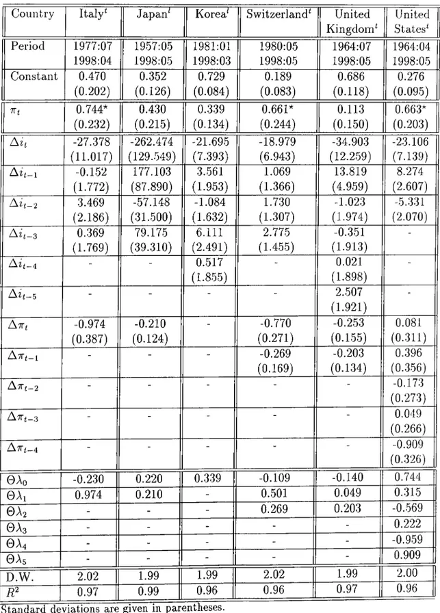
Table 4.2: Long-term Effect of Inflationary Expectations on the Nominal Interest Rate: Developed Countries
1 Country Belgium^ Canada* Denmark* Finland* France* Germany* 1 Period 1957:04 1998:05 1957:08 1998:05 1981:06 1988:12 1978:03 1998:04 1966:03 1998:05 1975:10 1998:05 1 Constant 0.392 (0.147) 0.225 (0.127) 0.339 (0.179) 0.275 (0.477) 0.218 (0.038) 0.264 (0.087)
1
(0.337)0.620* 0.98* (0.267) 1.302* (0.307) 0.963* (0.901) 0.465 (0.069) 0.814* (0.283) Ait -77.131 (37.914) -36.305 (10.468) -12.024 (4.417) -112.579 (104.659) -25.445 (5.369) -33.545 (12.017) 13.066 (7.145) 12.650 (3.934) - 10.412 (11.424) -1.925 (1.347) 8.613 (3.677) ^'h-2 0.440 (1.830) - 23.684 (22.263) - 4.183 (2.461) ^ h -3 “ -1.319 (1.880) “ “ - -Ait-4 “ -0.322 (1.832) “ “ - -" 1.722 (1.866) “ - - -A it-e “ -4.245 (2.203) - - - -A-Kt -0.268 (0.312) -0.663 (0.239) -1.288 (0.301) -1.159 (1.079) -0.306 (0.091) -0.429 (0.253) Ant-i 0.373 (0.367) “ -1.079 (0.268) -0.882 (0.842) -0.366 (0.098) -0.127 (0.223) A7Ti_2 “ “ -0.829 (0.227) “ -0.321 (0.091) 0.271 (0.233) A-Kt-3 “ -0.483 r0.180) “ ATTt-4 -0.306 (0.144) “ ■ 0Ao 0.352 0.315 0.015 -0.197 0.159 0.385 0Ai 0.641 0.663 0.209 0.277 -0.060 0.3020
A2
-0.373 - 0.249 0.882 0.045 0.3980
A3
- - 0.337 - 0.321 -0.2710
A4
- - 0.187 - - -0As - - 0.305 - - ' D.W. 1.99 2.00 1.87 2.00 2.00 1.99 R? 0.99 0.98 0.98 0.98 0.99 0.98* Do not reject the null hypothesis: F = 1 at the 5% significance level. ^ Treasury bill rate is used to model the interest rate.
^ Lending rate is used to model the interest rate. Inflation rate is modeled based on the CPI.
CHAPTER 4. ESTIMATION AND RESULTS 20
Table 4.3: Long-term Effect of Inflationary Expectations on the Nomiiicil Interest Rate: Developed Countries continued
Country Italy' Japan' Korea' Switzerland' United Kingdom^ United States' Period 1977:07 1998:04 1957:05 1998:05 1981:01 1998:03 1980:05 1998:05 1964:07 1998:05 1964:04 1998:05 Constant 0.470 (0.202) 0.352 (0.126) 0.729 (0.084) 0.189 (0.083) 0.686 (0.118) 0.276 (0.095) 0.744* (0.232) 0.430 (0.215) 0.339 (0.134) 0.661* (0.244) 0.113 (0.150) 0.663* (0.203) A i t -27.378 (11.017) -262.474 (129.549) -21.695 (7.393) -18.979 (6.943) -34.903 (12.259) -23.106 (7.139) A i t - i -0.152 (1.772) 177.103 (87.890) 3.561 (1.953) 1.069 (1.366) 13.819 (4.959) 8.274 (2.607) A i t - 2 3.469 (2.186) -57.148 (31.500) -1.084 (1.632) 1.730 (1.307) -1.023 (1.974) -5.331 (2.070) ^ h - 3 0.369 (1.769) 79.175 (39.310) 6.111 (2.491) 2.775 (1.455) -0.351 (1.913) A z^_4 - " 0.517 (1.855) “ 0.021 (1.898) ■ - - “ " 2.507 (1.921) ■ A w i -0.974 (0.387) -0.210 (0.124) “ -0.770 (0.271) -0.253 (0.155) 0.081 (0.311) A v t - i - - “ -0.269 (0.169) -0.203 (0.134) 0.396 (0.356) A - K t - 2 - “ “ “ -0.173 (0.273) AT Tt-3 - - " “ ■ 0.049 (0.266) ATTt-4 - - “ “ -0.909 (0.326) 0 A o -0.230 0.220 0.339 -0.109 -0.140 0.744 0 A i 0.974 0.210 - 0.501 0.049 0.315 0A2 - - - 0.269 0.203 -0.569 0A3 - - - 0.222 0A4 - - - -0.959 0 A s - - - 0.909 D.W. 2.02 1.99 1.99 2.02 1.99 2.00 B ? 0.97 0.99 0.96 0.96 0.97 0.96
* Do not reject the null hypothesis: T = 1 at the 5% significance level. * Treasury bill rate is used to model the interest rate.
^ Lending rate is used to model the interest rate. Inflation rate is modeled based on the CPI.
CHAPTER 4. ESTIMATION AND RESULTS
21
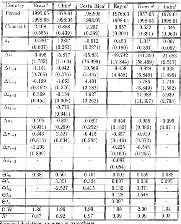
Table 4.4: Long-term Effect of Inflationary Expectations on the Nominal Interest Rate: Developing Countries
Country Brazil' Chile' Costa Rica' Egypt' Greece' India' Period 1995:05 1998:03 1978:01 1998:05 1982:05 1998:05 1976:03 1998:04 1957:05 1998:05 1979:04 1998:01 Constant 2.408 (0.555) 0.888 (0.439) 2.267 (0.392) 0.857 (0.204) 0.632 (0.391) 1..345 (0.063) TTi -0..381* (0.807) 1.385* (0.263) -0.012 (0.227)) 0.453 (0.190) 1.01* (0..391) 0.007 (0.062) A i t -3.495 (1.782) -5.877 (1.163) -35.831 (16.999) -49.742 (17.844) -141.359 (58.469) -21.683 (9.517) A i t - i -1.151 (0.766) 0.942 (0.376) 10.569 (5.447) -9.458 (4.458) -0.928 (6.849) 0.335 (1.496) A i t - 2 -0.169 (0.462) -1.063 (0.376) 4.401 (3.281) - 5.786 (6.849) 1.746 (1.582) A i t - 3 0.569 (0.455) -0.154 (0.308) 4.927 (3.262) - 21.988 (11.307) 5.939 (2.708) A i t - 4 “ -0.776 (0.341) - -A lT t 0.405 (0.931) -0.824 (0.299) -0.092 (0.252) -0.454 (0.182) -0.955 (0.386) -0.095 (0.071) A T T t - i 0.343 (0.815) 2.527 (0.634) -0.415 (0.285) -0.357 (0.146) -0.919 (0.372) -A ' K t - 2 -1.203 (0.899) “ - -0.225 (0.100) -0.548 (0.255) -A ' K t - 3 “ “ -0.097 (0.054) “ 0 A o -0.381 0.561 -0.104 -0.001 0.059 -0.088 0 A i - 3.351 -0.324 0.097 0.036 0.095 0 A2 - -2.527 0.415 0.132 0.371 -0 A3 - - - 0.128 0.548 -0 A4 - - - 0.097 - -D.W. 1.80 1.99 1.99 1.99 2.00 1.94 R^ 0.87 0.92 0.97 0.99 0.99 0.93
* Do not reject the null hypothesis: F = 1 at the 5% significance level. * Treasury bill rate is used to model the interest rate.
‘ Lending rate is used to model the interest rate. Inflation rate is modeled based on the CPI.
CHAPTER 4. ESTIMATION AND RESULTS 22
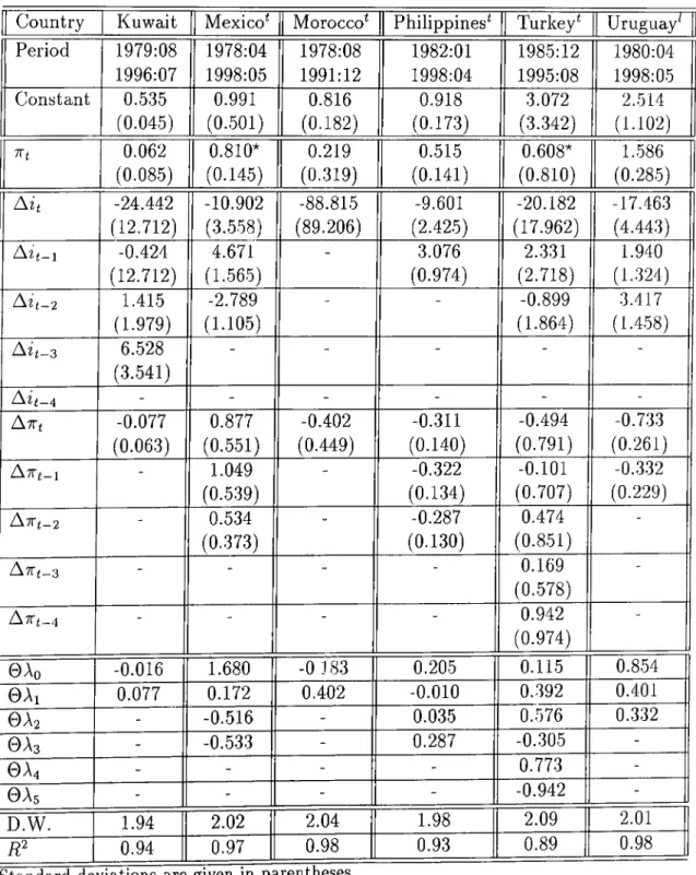
Table 4.5: Long-term Effect of Inflationary Expectations on the Nominal Interest Rate: Developing Countries continued
Country Kuwait Mexico* Morocco* Philippines* Turkey* Uruguay* Period 1979:08 1978:04 1978:08 1982:01 1985:12 1980:04 1996:07 1998:05 1991:12 1998:04 1995:08 1998:05 Constant 0.535 0.991 0.816 0.918 3.072 2.514 (0.045) (0.501) (0.182) (0.173) (3.342) (1.102) 0.062 0.810* 0.219 0.515 0.608* 1.586 (0.085) (0.145) (0.319) (0.141) (0.810) (0.285) Nit -24.442 -10.902 -88.815 -9.601 -20.182 -17.463 (12.712) (3.558) (89.206) (2.425) (17.962) (4.443) ^'h-1 -0.424 (12.712) 4.671 (1.565) - 3.076 (0.974) 2.331 (2.718) 1.940 (1.324) Nit-2 1.415 (1.979) -2.789 (1.105) “ “ -0.899 (1.864) 3.417 (1.458) Nit-3 6.528 (3.541) “ “ “ “ “ Nit-4 - - - -Nwt -0.077 0.877 -0.402 -0.311 -0.494 -0.733 (0.063) (0.551) (0.449) (0.140) (0.791) (0.261) NTTt-l - 1.049 (0.539) - -0.322 (0.134) -0.101 (0.707) -0.332 (0.229) NlTt-2 - 0.534 (0.373) - -0.287 (0.130) 0.474 (0.851) “ N i T t - s - - “ " 0.169 (0.578) NTTt-4 - “ “ 0.942 (0.974) 0Ao -0.016 1.680 -0 183 0.205 0.115 0.854 0Ai 0.077 0.172 0.402 -0.010 0.392 0.401
0
A2
- -0.516 - 0.035 0.576 0.3320
A3
- -0.533 - 0.287 -0.305-0
A4
- - - - 0.773 -0As - - - - -0.942 -D.W. 1.94 2.02 2.04 1.98 2.09 2.01 R^ 0.94 0.97 0.98 0.93 0.89 0.98* Do not reject the null hypothesis: T = 1 at the 5% significance level. * Treasury bill rate is used to model the interest rate.
^ Lending rate is used to model the interest rate. Inflation rate is modeled based on the CPI.
CHAPTER 4. ESTIMATION AND RESULTS 23
Table 4.6; Long-term Effect of Inflationary Expectations on the Nominal Interest Rate: Developing Countries continued
I Country Venezuela^ Zambia* 1 Period 1984:07 1985:02 1998:04 1998:01 1 Constcint 1.167 0.092 1 (1.094) (2.114) 1 0.4.51* 0.727* 1 ( 0..3.36) (0.409) lS.it -34.325 -22.876 (20.484) (9.715)
2
.4.33
10.286 (3.003) (4.638) Az'i_2 1.463 5.012 (2.758) (2.713) -3.199 -5.921 (3.446) (3.361) Az^_4 - -ATTi 0.849 (0.666) -A7Ti_i - -A7Ti_2 - -A7Ti_3 - -0Ao 1.300 0.727 0Ai -0.849-0
A2
--0
A3
--0
A4
- -D.W. 2.02 2.04 0.96 0.96Standard deviations are given in parentheses.
* Do not reject the null hypothesis: F = 1 at the 5% significance level. * Treasury bill rate is used to model the interest rate.
^ Lending rate is used to model the interest rate. Inflation rate is modeled based on the CPI.
CHAPTER 4. ESTIMATION AND RESULTS 24
The Durbin-Watson statistic is reported for all the models estimated in order to measure the serial autocorrelation. We employ further the Q-statistic test which test for more general forms of serial correlation than does the Durbin-Watson statistic. Besides, we performed the ARCH-LM test in order to detect for autoregressive conditional heteroskedasticity. In addition to that, we performed the Chow Breakpoint test in order to check whether there is any structural change or not. These robustness analysis is provided in the following subsection.
Examining Table 4.2 through Table 4.6 we foud that for the twenty six countries examined, our results revealed that there is no evidence to reject the Fisher hypothesis for fifteen countries. That is the null hypothesis of F = 1 can not be rejected for fifteen countries. Thus the strong version of the Fisher hypothesis tends to hold for slightly more than half of the times. Among the developed countries, we did not find any evidence to reject the strong version of the Fisher hypothesis for Belgium, Canada, Denmark, Finland, Germany, Italy, Switzerland, and United States. Whereas, among the developing ones, we did not find any evidence to reject the strong version of the Fisher hypothesis for Brazil, Chile, Greece, Mexico, Turkey, Venezuela, and Zambia.
Concerning the developed countries our results are in line with those performed by Moazzami [31]. There is no evidence for rejecting the long- run Fisher effect for United States, Canada, Italy, and Germany, but not for the United Kingdom. The only conflicting result of our study with that of Moazzami [31], is the one related to France.
For the twelve developed countries examined in our study, we encountered partial adjustment of the nominal interest rate to expected inflation for three
CHAPTER 4. ESTIMATION AND RESULTS 25
countries: France, Japan and Korea. Whereas we encountered no adjustment at all for only one country: United Kingdom. Full adjustment of the nominal interest rate to expected inflation is observed for eight countries: Belgium, Canada, Denmark, Finland, Germany, Italy, Switzerland, and United States.
Whereas, the developing countries which did not attract much attention in the literature, we found that there is a tendency for the Phsher hypothesis to hold for Mexico, in line with the result reported by Thornton [-39].
For the fourteen developing countries examined in our study, partial adjustment of the nominal interest rate to expected inflation is encountered for four countries: Egypt, Morocco, Philippines, and Uruguay. No adjustment at all was encountered by three countries: Costa Rica, India, and Kuwait. Full adjustment of the nominal interest rate to expected inflation is observed for five countries: Brazil, Chile, Greece, Mexico, Turkey, Venezuela and Zambia.
In fact, the main difference between the developed and the developing countries is the degree of the deregulation of the financial system. Usually, the developing countries are characterized by restrictions on free movements of financial asset prices associated with market regulation of interest and exchange rate. Thus it is more likely that the F’isher hypothesis does not hold. This is due to Olekalns [33] who suggested that the Fisher hypothesis tends to hold in a financially deregulated economy. So, it is expected that a few or none of the developing countries will exhibit the Fisher effect. In fact this is not the case, since we have detected that half of the time the Fisher effect is holding for the developing countries. Furthermore, these countries have already started the deregulation process which was nicely reflected in the sample period that we have examined. Thus after deregulation, the real interest rate tend to be
CHAPTER 4. ESTIMATION AND RESULTS 26
steadier since the nominal rates of return are free to adjust rapidly to expected inflation movements.
In fact the degree of interest rates control can be one of the explanations of having the Fisher hypothesis tending to hold with more chance in the developed countries than in the developing ones.
The short-run dynamics of the nominal interest rate to the expected inflation rate are reported in Table 4.2 through Table 4.6. Examining the countries where the Fisher hypothesis tend to hold, we conclude that the short-run responses of the nominal interest rate to expected inflation does not display a consistent pattern among countries. In fact the adjustment process differs from one country to another. However, an interesting point is that for some of the developing countries, the short-run adjustment of the nominal interest rate to expected inflation is more than proportional, in particuhu’, Chile, Mexico, and Venezuela. In contrast, for the developed countries, the short-run adjustment of the nominal rate to expected inflation is always less than proportional.
CHAPTER 4. ESTIMATION AND RESULTS 27
4.1.3
Robustness Analysis
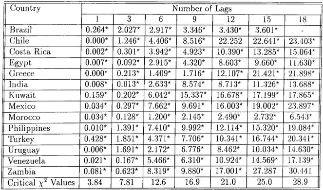
The Ljung-Box Q statistic tests for serial correlation are performed. The Q- statistic is used to test the null hypothesis that all of the autocorrelations are zero; In other words the series is white noise. The Q-statistics are calculated for different number of lags and for all countries under study. These are reported in the following tables:
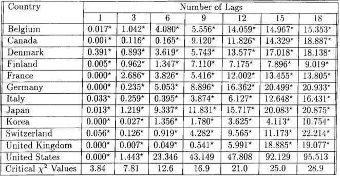
Table 4.7: The Q-statistics: F-values for the developed countries Country Number of Lags
1 3 6 9 12 15 18 Belgium 0.017* 1.042* 4.080* 5.556* 14.059* 14.967* 15.353* Canada 0.001* 0.116* 0.165* 9.120* 11.826* 14.329* 18.887* Denmark 0.391* 0.893* 3.619* 5.743* 13.577* 17.018* 18.138* Finland 0.005* 0.962* 1.347* 7.110* 7.175* 7.896* 9.019* France 0.000* 2.686* 3.826* 5.416* 12.002* 13.455* 13.805* Germany 0.000* 0.235* 5.053* 8.896* 16.362* 20.499* 20.933* Italy 0.033* 0.259* 0.395* 3.874* 6.127* 12.648* 16.431* Japan 0.013* 1.219* 9.337* 11.831* 15.717* 20.083* 20.875* Korea 0.000* 0.027* 1.356* 1.780* 3.625* 4.113* 10.754* Switzerland 0.056* 0.126* 0.919* 4.282* 9.565* 11.173* 22.214* United Kingdom 0.000* 0.007* 0.049* 0.541* 5.991* 18.885* 19.077* United States 0.000* 1.443* 23.346 43.149 47.808 92.129 95.513 Critical x'^ Values 3.84 7.81 12.6 16.9 21.0 25.0 28.9
Do not reject that all of the autocorrelations are zero at the 5% significance level
Examining Table 4.7 we notice that the null hypothesis that all of the autocorrelations are zero is rejected for all the developed country models that we have estimated, except that for the United States. Thus except for the case of the United States no autocorrelation problem is faced. The case of the United States will be handled in the forthcoming analysis.
CHAPTER 4. ESTIMATION AND RESULTS 28
is tested for the developing country models. The F-values for such a test are reported in Table 4.8.
Table 4.8; The Q-statistics: F-values for the developing countries Country Number of Lags
9 12 15 18 Brazil 0.264* 2.027* 2.917* 3.346* 3.430* 3.601* Chile 0.000* 1.246* 4.406* 8.516* 22.252 22.641* 23.403* Costa Rica 0.002* 0.301* 3.942* 4.923* 10.390* 13.285* 5.064* Egypt 0.007* 0.092* 2.915* 4.320* 8.603* 9.660* 11.630* Greece 0.000* 0.213* 1.409* 1.716* 12.107* 21.421* 21.898* India 0.008* 0.013* 2.633* 8.574* 8.713* 11.326* 13.688* Kuwait 0.159* 0.202* 6.042* 15.337* 16.678* 17.199* 17.865* Me.xico 0.034* 0.297* 7.662* 9.691* 16.003* 19.002* 23.897* Morocco 0.034* 0.128* 1.200* 2.145* 2.490* 2.732* 6.543* Philippines 0.010* 1.391* 7.410* 9.992* 12.114* 15.320* 19.084* Turkey 0.428* 1.851* 4.371* 7.706* 10.341* 16.744* 20.341* Uruguay 0.006* 1.691* 2.172* 6.776* 8.462* 10.034* 14.630* Venezuela 0.0 2 1* 0.167* 5.466* 6.310* 10.924* 14.569* 17.139* Zcimbia 0.081* 0.623* 8.319* 9.880* 17.001* 27.287 30.441 Critical Values 3.84 7.81 12.6 16.9 21.0 25.0 28.9 * Do not reject that all of the autocorrelations are zero at the 5% significance level.
Examining Table 4.8, no autocorrelation is encountered for all the estimated models of the developing countries.
In fact for all the country models that we have come up with, we did not encounter any autocorrelation problem, except for the case of the United States. For United States’ model the null hypothesis that all the autocorrelations are zero can not be rejected at the 5% significance level when at least six lags of the residuals are considered. Whereas, for one and three lags of the residuals, no autocorrelation is encountered.
CHAPTER 4. ESTIMATION AND RESULTS 29
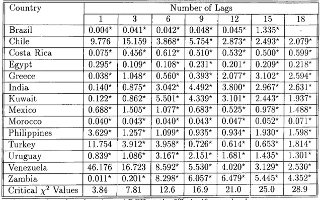
In addition to the test of residual autocorrelation, the ARCH-LM pi'ocedure is performed in order to test for autoregressive conditional heteroskedasticity (ARCH ). The test consists of regressing the m odel’s squared residuals on lagged squared residuals. The null hypothesis that the coefficient of the lagged squared residuals are all zero, is then tested against the alternative hypothesis that at least one of the coefficients of the lagged squared residual is different from zero. For this purpose, the F-statistics for different number of lagged squared residuals, and for all the countries under study are calculated, and compared to the corresponding critical value. If the F-statistic is less than the corresponding x'^ critical value, then there is no evidence of rejecting the null hypothesis of no ARCH. All the calculated F-values for the different country models under study and for different number of residual lags are reported in Table 4.9, and Table 4.10.
Table 4.9: The ARCH-LM test: F-values for the developed countries Country Number of Lags
1 3 6 9 12 15 18 Belgium 8.063 5.496* 3.068* 2.086* 1.648* 1.302* 1.084* Canada 3.819* 4.932* 2.843* 14.880* 12.615* 10.500* 9.104* Denmark 0.000* 0.129* 0.106* 0.267* 0.246* 0.375* 0.359* Finlcind 9.560 4.088* 2.455* 2.264* 1.833* 1.478* 1.410* France 0.002* 0.080* 0.089* 0.122* 2.727* 2.158* 1.775* Germany 0.130* 3.083* 2.400* 2.764* 2.384* 2.006* 1.713* Italy 8.904 3.627* 2.072* 1.401* 1.077* 1.170* 1.145* .Japan 87.936 65.615 50.008 34.458 26.031 20.586* 16.965* Korea 3.703* 3.063* 1.563* 1.027* 0.763* 0.606* 2.026* Switzerland 10.298 6.572* 5.885* 4.736* 5.227* 4.628* 3.969* United Kingdom 34.777 13.643 8.275* 5.652* 4.239* 3.407* 2.858* United States 118.858 49.505 33.056 22.708 18.832* 15.486* 13.795* Critical x^ Values 3.84 7.81 12.6 16.9 21.0 25.0 28.9
Do not reject that there is no ARCH at the 5% significance level.
CHAPTER 4. ESTIMATION AND RESULTS 30
heteroskedasticity is detected for the models of Canada, Denmark, France, Germany and Korea. Whereas, for the model of Belgium, Finland, Italy, and Switzerland, autoregressive conditional heteroskedasticity is detected for only one lag of the squared residuals. However, for the case of the United States and .Japan autoregressive conditional heteroskedasticity is detected for most of the lags of the squared residuals included.
Similarly the the null hypothesis that the coefficient of the lagged squared residuals are all zero, that is there is no ARCH for the developing country models is tested. The F-values for such a test are reported in Table 4.10.
Table 4.10: The ARCH-LM test: F-values for the developing countries Country Number of Lags
1 3 6 9 12 15 18 Brazil 0.004* 0.041* 0.042* 0.048* 0.045* 1.335* -Chile 9.776 15.159 3.868* 5.754* 2.873* 2.493* 2.079* Costa Rica 0.075* 0.456* 0.612* 0.510* 0.532* 0.500* 0.599* Egypt 0.295* 0.109* 0.108* 0.231* 0.201* 0.209* 0.218* Greece 0.038* 1.048* 0.560* 0.393* 2.077* 3.102* 2.594* India 0.140* 0.875* 3.042* 4.492* 3.800* 2.967* 2.631* Kuwait 0.122* 0.862* 5.501* 4.339* 3.101* 2.443* 1.937* Mexico 0.688* 1.505* 1.077* 0.683* 0.525* 0.978* 1.488* Morocco 0.040* 0.043* 0.040* 0.043* 0.047* 0.052* 0.071* Philippines 3.629* 1.257* 1.099* 0.935* 0.934* 1.930* 1.598* Turkey 11.754 3.912* 3.958* 0.726* 0.61-4* 0.653* 1.814* Uruguay 0.839* 1.086* 3.167* 2.151* 1.681* 1.435* 1.301* Venezuela 46.176 16.723 8.592* 5.530* 4.020* 3.129* 2.530* Zambia 0.011* 0.201* 8.298* 6.057* 6.479* 5.445* 4.352* Critical Values 3.84 7.81 12.6 16.9 21.0 25.0 28.9
Do not reject that there is no ARCH at the 5% significance level.
Examining Table 4.10, we notice that for the developing countries, most of the models do not reveal any autoregressive conditional heteroskedasticity, except for the case of Venezuela, and Turkey. For the case of Turkey, ARCH
CHAPTER 4. ESTIMATION AND RESULTS 31
process is detected just when one lag of the squared residuals is included. Whereas, for the case of Venezuela, ARCH process is detected when one and three lags of the squared residuals are included.
In fact for all the country model that we have estimated, we detected the ARCH process for Belgium, Finland, Italy, Jap<m, Switzerland, United Kingdom, llnited States, Turkey and Venezuela.
CHAPTER 4. ESTIMATION AND RESULTS 32
In addition to testing our models for any serial autocorrelation and for the ARCH process, we have tested them for structural changes. For this purpose, the Chow Breakpoint test is carried out in order to detect whether our estimated models reveal a any structural change or not. In order to perform this test the breakpoint is needed. For this purpose we have examined all the key economic policy events for each country.
For the Fhiropean countries: Belgium, France, Germany, Italy (formed the core of the European Economic Community (EEC) in 1957), Denmark, United Kingdom ( joined the EEC in 1973), and Finland (joined the European Union in 1995), we have examined the following dates, whenever included in the country’s sample period, as possible structural breakpoints:
• 1967:06 The general agreement on Tariffs and Trade is finally concluded and signed.
• 1974:03 The oil price crisis.
• 1979:03 The European Monetary System (EMS) is launched to protect the European Union Currencies from wild exchange rate fluctuations.
• 1987:07 The Single European Act comes into force.
• 1992:02 The Maastricht Treaty is signed by the European Union members.
• 1993:01 The single European market comes into force.
In addition to that for the case of Germany the unification date, 1990:10 was also examined. Whereas, for Switzerland which is not a member of the EU, random breakpoint dates were chosen.
CHAPTER 4. ESTIMATION AND RESULTS 33
For the North American countries: Canada, the oil price crisis (1974:03), the Free Trade Agreement (FTA) with the United States (1989:06), and the North American Free Trade Agreement (NAFTA) with the United States and Mexico (1994:06) were examined. For the United States, the oil price crisis (1974:03), and the main recession date lived by the economy (1978:01, 1981:01, 1983:01, 1990:01), and a recovery date (1994:01) were examined. For the East Asicin countries: .Japan, the oil price crisis (1974:03), the opening of the Japan’s domestic market to foreign imports (1990:01), the financial crisis (1997:06), and for Korea, the reduction in government controls (1990:01), the financial crisis (1997:06), were examined. Concerning the developing countries most of the breakpoints considered are those referring to the deregulation procedures, the openness of the economy, the trade liberalization, the economic reforms etc. The statistics of the Chow Breakpoint test are reported in the following tables.
la b le 4.11: The Chow Breakpoint Test: F-statistics, Probcibilities for the develoi^ed countries Country Sample Period Break Point F-statistic Probability Belgium 1957:04 1998:05 1967:06 0.000813 1.00 1974:03 0.000704 1.00 1979:03 0.001461 1.00 1987:07 0.000361 1.00 1992:02 0.000506 1.00 1993:01 0.000670 1.00 Canada 1957:08 1998:05 1974:03 0.000146 1.00 1989:06 0.000007 1.00 1994:06 0.000686 1.00 Denmark 1981:06 1988:12 1987:07 0.001758 1.00 Finland 1978:03 1998:04 1979:03 0.000132 1.00
CHAPTER 4. ESTIMATION AND RESULTS 34
Table 4.12: The Chow Breakpoint Test: F-statistics, Probabilities for the developed countries continued
Country Sample Period Break Point F-statistic Probability France 1966:03 1998:05 1974:03 0.005565 1.00 1979:03 0.003670 1.00 1987:07 0.000730 1.00 1992:02 0.000745 1.00 1993:01 0.001026 1.00 Germany 1975:10 1998:05 1979:03 0.001824 1.00 1987:07 0.001824 1.00 1987:07 0.000770 1.00 1990:10 0.001075 1.00 1992:02 0.001516 1.00 1993:01 0.002393 1.00 Italy 1977:07 1998:04 1979:03 0.001238 1.00 1987:07 0.000662 1.00 1992:02 0.000711 1.00 1993:01 0.005760 1.00 Japan 1957:05 1998:05 1974:03 0.000059 1.00 1990:01 0.000216 1.00 1997:06 0.000002 1.00 Korea 1981:01 1998:03 1990:01 0.005911 1.00 1997:06 0.029717 0.99 Switzerland 1980:05 1998:05 1985:01 0.004114 1.00 1990:01 0.002281 1.00 1995:01 0.003560 1.00 United Kingdom 1964:07 1998:05 1974:03 0.001015 1.00 1979:03 0.002162 1.00 1987:07 0.001059 1.00 1992:02 0.000572 1.00 1993:01 0.000380 1.00 United States 1964:04 1974:03 1.345198 0.20 1998:05 1978:01 1.675364 0.08 1981:01 3.447023 0.00 1983:01 2.807728 0.00 1990:01 1.662138 0.09 1994:01 0.676337 0.75 1981:01 1990:01 2.922382 0.00
CHAPTER 4. ESTIMATION AND RESULTS 35
Table 4.13: The Chow Breakpoint Test: F-statistics, Probabilities for the developing countries Country Sample Period Break Point F-statistic Probability Bl'cizil 1995:05 1998:03 1996:01 0.140464 0.98 Chile 1978:01 1998:05 1991:01 0.041013 0.99 Costa Rica 1982:05 1998:05 1991:01 0.000440 1.00 Egypt 1976:03 1998:04 1991:03 0.000252 1.00 1996:01 0.000905 1.00 Greece 1957:05 1998:05 1974:03 0.000077 1.00 1981:01 0.000119 1.00 India 1997:04 1998:01 1990:01 0.003581 1.00 1991:01 0.003955 1.00 Kuwait 1979:08 1996:07 1981:01 0.001140 1.00 1990:01 0.000750 1.00 Mexico 1978:04 1998:05 1988:01 0.010515 1.00 1994:04 0.027295 0.99 Morocco 1978:08 1991:12 1985:01 0.002207 0.99 Philippines 1982:01 1998:04 1989:06 0.002931 1.00 1991:06 0.007340 1.00 1994:05 0.008837 1.00 Turkey 1985:12 1995:08 1993:01 0.008768 1.00 Uruguay 1980:04 1998:05 1985:01 0.004610 1.00 Venezuela 1984:07 1998:04 1988:01 0.001058 1.00 1992:01 0.000123 1.00 Zambia 1985:02 1998:01 1990:01 0.003805 1.00
CHAPTER 4. ESTIMATION AND RESULTS 36
Examining Table 4.11 and Table 4.12, we notice that all the developed countries’ models did not exhibit any structural change at the 5% significance level, except for the case of the United States, which exhibited two breakpoint changes. In fact the structural breakpoints stand for the recessions that characterized the American Economy at the early eighties and the early nineties.
Examining Table 4.13, we notice none of the developing country models exhibit any structural change at the 5% significance level.
So for all the country’s models we did not detect any structural change except for the case of the United States.
CHAPTER 4. ESTIMATION AND RESULTS 37
The structural change in the US model is taken into account and the models are reestimated for the corresponding sample periods. The results are provided in Table 4.15. The latter models did not show any serial autocorrelation problem. However, the ARCH process is detected for the first two sample periods, but no ARCH process for the third one. The detailed results of the Q-statistic test and the ARCH-LM procedure are provided in Table 4.14.
The Fisher hypothesis is still holding for all the three different sample periods. Thus the US data behaves in line with the Fisher hypothesis.
Table 4.14: Robustness Analysis for the US adjusted models United States Period 1974:01 1981:01 1981:01 1990:01 1990:01 1998:05 Lags Critical Values Q-statistics F-values 1 3.84 0.034* 0.359* 0.084* 3 7.81 0.254* 1.054* 4.097* 6 12.6 4.929* 8.206* 6.633* 9 16.9 8.785* 12.458* 13.755* 12 21.0 10.761* 13.909* 13.970* 15 25.0 16.803* 19.438* 20.566* 18 28.9 18.221* 20.897* 22.405* Lags Critical Values APICH-LM test F-values 1 3.84 45.693 5.908 0.000° 3 7.81 18.704 12.451 1.341° 6 12.6 9.169° 23.312 2.1.3° 9 16.9 6.369° 14.882 1.388° 12 21.0 5.155° 7.392° 1.494° 15 25.0 3.947° 5.469° 1.165° 18 28.9 3.494° 5.787° 0.998° * Do not reject that
° Do not reject that
all of the autocorrelations are zero at the 5% significance level, there is no ARCH at the 5% significance level.
CHAPTER 4. ESTIMATION AND RESULTS 38
Table 4.15: The adjusted models for the US data
Period United States 1974:01 1981:01 1981:01 1990:01 1990:01 1998:05 Constant 0.222 (0.779) 0.429 (0.137) 0.402 (0.187) 0.777* (0.985) 0.5734* (0.361) -0.132* (0.771) Ait -34.477 (74.804) -11.924 (4.905) -46.964 (31.046) ^'h-1 20.754 (42.145) 1.203 (1.159) 20.303 (14.063) Ait-2 -16.775 (37.244) -2.108 (1.394) 5.986 (6.103) A i t - 3 “ 1.208 (1.154) “ A i t - 4 - -2.914 (1.476) - 3.348 (1.810) -Awt 1.145 (3.779) 0.305 (0.526) -0.009 (0.665) Awt-i 1.743 (4.732) 0.103 (0.411) 0.433 (0.749) ATTt-2 0.767 (2.574) -0.102 (0.330) 0.698 (0.795) A i T t - s 0.606 (2.061) -0.241 (0.275) 0.087 (0.441) A % t - 4 -2.719 (5.591) -0.801 (0.342) 0.089 (0.351) 0Ao 1.922 0.879 -0.141 0Ai 0.597 -0.203 0.442
0
A2
-0.975 -0.204 0.264 0 A3 -0.161 -0.139 -0.6110
A4
-3.326 -0.560 0.003 0A.5 2.719 0.802 -0.089 D.W. 1.95 1.88 2.04 0.94 0.96 0.99 significance level.Chapter 5
Conclusion
5.1
Conclusion
There is a long tradition of testing the Fisher hypothesis. In this study we tried to extend the available literature by examining the Fisher hypothesis for a sample of countries using the method suggested by Moazzami [30]. The latter models the Fisher hypothesis within a framework that cillows direct estimate of the long run coefficients, while taking into consideration the short run dynamics.
In this work we focused our attention on testing the strong version of the Fisher hypothesis under the case of before tax interest rates. That is does the nominal interest rate rise point-for-point to the expected inflation?
In testing the Fisher hypothesis for different countries we come out with the following results. First among the developed countries studied we have encountered that the long run Fisher effect tends to hold for 67% of all the
CHAPTER 5. CONCLUSION 40
studied cases. Whereas, for the developing ones, the long run Fisher effect tends to hold for 50% of all the studied cases. Thus, we can neither say that the Fisher hypothesis does always hold nor the Fisher hypothesis does not hold at all. In fact the major implication is that the Fisher hypothesis must be tested by the policymakers in order to decide on targeting the nominal or the real interest rate in hopes of influencing the real business cycle. If the Fisher hypothesis holds than it is more likely that real interest rates don’t move in response to expected inflation, and thus inflationary movements are totally absorbed in nominal interest rates.
Second, the Fisher hypothesis is more likely to hold for the developed countries than for the developing ones. In addition to that among the developing countries, the Fisher effect tends to hold for the countries which have higher degree of financial market deregulations. In fact, the degree of financial deregulation has one of the major effects on allowing the Fisher effect to hold or not. Removing the restrictions on the free movement of financicil asset prices, and allowing market deregulation of interest and exchange rate results in a steadier real rate, as nominal rates of return are free to adjust rapidly to expected inflation movements.
Bibliography
[1] Amsler C. E., (1986), The Fisher Effect: Sometimes Inverted, Sometimes Not?. Southern Economic Journal^ 832-835.
[2] Atkins F. J., (1989), Cointegration, Error Correction and the Fisher Effect.
Applied Economics^ 21, 1611-1620.
[3] Barth J., and Bradley M., (1988), On Interest Rates, Inflationary Expectations and Tax Rates. Journal of Banking and Finance^ 12, 215-
220
.[4] Bewley R. A., (1979), The Direct Estimation of the Equilibrium Response in a Linear Dynamic Model. Economic Letters, 3, 4, 357-361.
[5] Boudoukh J., and Richardson M., (1993), Stock Returns and Inflation: A Long-horizon Perspectives. American Economic Review, 83, 1346-1355.
[6] Carmichael J. and Stebbing P. W ., (1983), Fisher’s Paradox and the Theory of Interest. American Economic Review, 73, 4, 619-630.
[7] Engel R. F., and Granger C. W. J., (1987) Cointegration and Error Correction: Representation, Estimation, and Testing. Economet/rica, 55, 251-276.
[8] Fisher L, (1930), The Theory of Interest. Macmillan, New York.
BIBLIOGRAPHY 42
[9] Fried J. and Howitt P., (1983), The Effects of Inflation on Real Interest Rates. American Economic Review^ 73, 968-980.
[10] Gallagher M. ,(1986), The Inverted Fisher Hypothesis: Additional Evidence. American Economic Review, 76, 247-249.
[11] Garbade K., and Watchtel P., (1978), Time Variation in the Relationship between Inflation and Interest Rates. Journal of Monetary Economics, 4, 755-765.
[12] Garcia P., and Zapta H., (1991), Cointegration, Error Correction cind the Fisher Eiffect: A Clarification. Applied Economics, 23, 1367-1368.
[13] Gonzalo J., (1994) Five Alternative Methods of Estimating Long-run Equilibrium Relationships. Journal of Econometrics, 60, 203-233.
[14] Gordon R. J., (1971), Inflation in Recession and Recovery. Brookings papers Washington, 105-158.
[15] Gupta K. L., and Moazzami B., (1991), On Some Predictions of the Quantity Theory of Money. Southern Economic Journal, 1085-1091.
[16] Hamori S., (1997), A Simple Method to Test the Fisher Effect. Applied Economics Letters, 4, 477-479.
[17] Elansen L. P., (1982), Large Sample Properties of Generalized Method of Moments Estimators. Econometrica, 50, 1029-1054.
[18] Hawtrey K. M., (1997), The Fisher Effect and Australian Interest Rates.
Applied Financial Economics, 7, 337-346.
[19] Hsiao C., (1979), Causality tests in Econometrics. Journal of Economic Dynamics and Control, 1, 321-346.