- ) i ^ < I I i I ■ « I I i i; s I ’
V /
r
I f ' ' " I Í! i I ; ( f r 1 1 I *-r I f \ ! 1 1 . i r ( 1 t r * *ir
-1 Г ! i ■ .’ f > t i » i Z r * « Î и г »! ■ t 1 n 0 I f Í . i ! iC -j * · Î ^ __ " ■ / J \ il ; r ’ ' " t ' \ J i I I f rr^ :I·
;:
i ^ ' I' i i ' l * 1 t ‘ 1 ^ • 1 ^ ' I 1 ( « . 1 ( ‘ i Г . 1 * "Í ^ ( . > * i J i .■ ' Ш ^ . r · r. 1 Г ? ΐ τ 1 i Í Î У '" * » Í L ::. '.i . η i i.CALENDER ANOMALIES
AT
ISTANBUL STOCK EXCHANGE
A THESIS
SUBMITTED TO THE DEPARTMENT OF MANAGEMENT AND THE GRADUATE SCHOOL OF BUSINESS ADMINISTRATION
OF BILKENT UNIVERSITY
IN PARTIAL FULFILLMENT OF THE REQUIREMENTS FOR THE DEGREE OF
MASTER OF BUSINESS ADMINISTRATION
BY
__R T Ü R ^ Y Q ^
μ 6
■гяч о З я і д З З
I certify that I have read this thesis and in my opinion it is fully adequate, in scope- and in quality, as a thesis for the degree of Master of Business Administration.
Assist. Prof. GOlnur M. SENGÖL
I certify that I have read this thesis and in my opinion it is fully adequate, in scope and in quality, as a thesis for the degree of Master of Business Administration.
Assist. Prof. Can Simga MUGAN
I certify that I have read this thesis and in my opinion it is fully adequate, in scope and in quality, as a thesis for the degree of Master of Business Administration.
Assoc. Prof, ümit EROL
Approved for the Graduate School of Business Administration
' Î Û
ABSTRACT
Calendar Anomalies at Istanbul Stock Exchange
Turkay OKTAY MBA in Management
Supervisor : Assist,Prof. Gulnur SENGUL February 1993, 61 Pages
A securities market in which market prices fully reflect all relevant information is called efficient. The Weak Form Efficient Market Hypothesis claims that there should not be any consistent patterns in security returns.
In this study, the existence of return patterns which is a indicator of weak form inefficiency of the market, are analyzed in Istanbul Stock Exchange. The period covered is in between January 4, 1988 and December 31, 1992 and studies are done through dividing the sample period into two parts.
The results of the analysis indicate that Istanbul Stock Exchange Market tends to be inefficient as time goes. Significant Day of the Week and Weekend Effect are found in the 1990-1992 period. January Effect also exists in the market for the entire sample period. The reasons of effects do not fully explain the return patterns to exist which is also the same case in different security markets.
ÖZET
Istanbul Menkul Kıymetler Borsasinda Takvim Etkileri
Tûrkay OKTAY
Yüksek Lisans Tezi, isletme Enstitüsü Tez Yöneticisi : Assist.Prof. Gülnur SENGUL
Şubat 1993, 61 Sayfa
Hisse senedi fiyatlarinin bütün ilgili bilgiyi yansittigi hisse senedi piyasalari etkin olarak a d l andirilirlar. Zayif Pazar Etkinlik Hipotezi hisse senedi getirilerinde tutarli bir patern olamayacagini iddia eder.
Bu (palismada, piyasanin Zayif Pazar Etkinliğine sahip olmadiginin göstergesi olan getiri paternlerini İstanbul Menkul Kiymetler Borsasinda varolup olmadigi arastirilmistir. 4 Ocak 1988 ile 31 Aralik 1992 arasindaki dönem taranmis ve calismalar bu dönem ikiye bölünerek yapilmistir.
Analiz sonuçlari yillar geçtikçe İstanbul Menkul Kiymetler Borsasinin etkinsizlige doğru bir eğilime girdiğini göstermiştir. 1990-1992 periyodunda istatistiki olarak önemli Haftanin Günleri Etkisi ve Haftasonu Etkisi bulunmuştur. Bütün analiz periyodu süresincede Ocak Etkisi bulunmuştur. Etkilerin diğer dünya borsalarinda görülen oluşma nedenleri gene diğer borsalarda olduğu gibi İstanbul Menkul Kiymetler Borsasinda da getiri paternlerinin olusmasini tam olarak açiklayamamistir.
I would like to express my gratitude to Assistant Professor Gulnur SENGUL for her valuable supervision during the development of this thesis. I also wish to express my thanks to Assistant Professor Can Simga MUGAN and Associate Professor limit EROL for their helpful comments. I thank Ugur GULEN and Noyan NARIN for their enthusiastic encouragement.
ACKNOWLEDGEMENTS
Abstract Ozet Acknowledgement s Table of Contents List of Tables List of Figures I . Introduction
II. Review of Literature
A. Efficient Market Theory
B. Implications of an Efficient Market C. Forms of Efficient Market Hypothesis D. Tests About Market Efficiency
E. Usefullness of Historical Prices Weak-Form Tests
F. Return Patterns
G. Early Tests of Randomness
H. Recent Developments in Random Walk I. Emprical Tests of Market Efficiency
The Case for Turkey III. Data and Methodology
A. The Data B . Methodology IV. Findings
V. Discussions and Conclusions References Appendices TABLE OF CONTENTS iii iv V vi 1 4 4 6 8 8 10 11 12 14 18 22 22 23 28 32 36 XX 39 X V
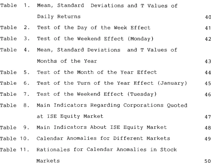
Table 1. Mean, Standard Deviations and T Values of
Daily Returns 40
Table 2. Test of the Day of the Week Effect 41 Table 3. Test of the Weekend Effect (Monday) 42 Table 4. Mean, Standard Deviations and T Values of
Months of the Year 43
Table 5. Test of the Month of the Year Effect 44 Table 6. Test of the Turn of the Year Effect (January) 45 Table 7. Test of the Weekend Effect (Tuesday) 46 Table 8. Main Indicators Regarding Corporations Quoted
at ISE Equity Market
47
Table 9. Main Indicators About ISE Equity Market 48 Table 10. Calendar Anomalies for Different Markets 49 Table 11. Rationales for Calendar Anomalies in Stock
Markets 50
LIST OF TABLES
LIST OF FIGURES Figure 1 . Figure 2. Figure 3. Figure 4. Figure 5. Figure 6. Figure 7 . Figure 8. Figure 9. Figure 10. Figure 1 1 . 4 . Jan,.1988--5. Oct.1 990 51 8 . Oct.,1990--31 . Dec . 1 992 52 4 . Jan.1 988--31 . Dec . 1 992 53 4 . Jan.1988--31 . Dec . 1 992 54 4 . Jan.1988--5 .Oct.1 990 55 8,. Oct.1990-■31 . Dec .1992 56 4,. Jan.1 988- 31 . Dec . 1 992 57 4. Jan.1 988- 31 . Dec . 1 992 58 Trading Vol ume 1986-88 59 Equiti es Traded 1986-88 60 Capitaliza tion 1986-88 61
I .INTRODUCTION
In modern economies, financial assets arise due to the need for financing excess of investment over saving, because savings are usually not equal to investment in real assets for all economic units in an economy over all periods of time.
The purpose of financial markets is to allocate savings efficiently to ultimate users. The more diverse the patterns of desired savings and investment among economic units, the greater the need for efficient financial markets to channel savings to ultimate users. The ultimate investor in real assets and the saver should be brought together at the least possible cost and inconvenience (Van Horne [22]).
The market for common stocks constitutes an important part of the financial markets. Besides being the basic source of long term equity financing for corporations, it can provide even very short term investment opportunities for individual investors.
If securities markets are efficient, prices will reflect all known information. As a result, prices will change only as new information arrives. But, by definition, new information will be random. If information flows followed an identifiable trend, this trend will become known and thus be reflected in current prices. Thus, new information must be random. And since new information enters randomly and prices react instantaneously to the information, changes in stock prices will be random
(Robert Radcliffe [20]).
economic signals which the market receives, then they can also be looked to provide useful signals to both suppliers and users of capital, the former for the purposes of constructing their investment portfolios, and the latter for establishing criteria for the efficient disposition of funds at their disposal. Lack of confidence in the pricing efficiency of the market tends to focus the attention of both investors and raisers of capital on potentially wasteful techniques of exploiting perceived inefficiencies, and away from a more positive recognition of the messages contained in the market's prices (Keane [17]).
In an efficient market, security prices follow what is referred as a random walk. A price rise on day 0 doesn't increase or decrease the odds of a price on day 1, day 2, etc. Price changes on any particular day are uncorrelated with historical price changes. If the random walk hypothesis is valid there should not be any consistent patterns in security returns.
The aim of this study is to analyze the existence of return patterns in Turkish Security Market and institutional factors underlying these patterns.
This study covers the five year period from January 1988 to December 1 992. In part II of this study the concept and implications of efficients market are summarized. Part II also contains early tests of randomness and relevant literature of recent studies about calendar anomalies on security returns. In part III, an explanation of the sample and methodology used in analyzing the return patterns is given. Daily returns are regressed against returns of the market to find systematic
anomalies including day of the week, weekend, months and turn of the year. Findings of analysis and major differences of results of two periods are given in Part IV. Part V includes conclusions, suggestions for further research and shortcomings of the study.
II. REVIEW OF LITERATURE
A. EFFICIENT MARKET THEORY
Efficient Market Theory (EMT) states that the security market is a fair game : the odds of having a future return greater than should be expected given a security's risk are the same as the odds of having a lower return than should be expected. There is no way to use the information available at a given point in time in order to earn an abnormal return. Positive returns will be expected, of course, because securities contain risk for which a risk premium will be earned. However, long-run abnormal returns will be zero (Radcliffe [20]).
Security prices are determined by expectations of future economic profits, risks, and interest rates. In developing such expectations, individuals assess any information which is available at that time. While list of relevant information is almost endless, the point is that such information is crucial to making a pricing decision. It is in this sense that theorists can say that security prices migth fully reflect all relevant information. A securities market in which market prices fully reflect all known information is called "efficient".
Paradoxically, security markets can be efficient only if a large number of people disagree with the EMT and attempt to find ways of earning speculative profits. To make a speculative profit, an individual must hold unique information about a security which other market participants are unaware of. As soon
as new information is obtained, speculators who have the information will immediately trade. If the speculators discover favorable information, they will immediately sell. As a result, profit maximizing speculators will attempt to obtain information before other market participants. This results in a race for new information and, at the extreme, all information will be reflected in security prices as soon as it becomes available.
The term price efficient is used to indicate that security markets are efficient in processing information. Prices will not adjust to new information with a lag but, instead,
1
instantaneously. Four conditions are necessary to have such an efficiently priced market :
1 . Information is costless and available to all market participants at the same point in time. (Participants have homogenous expectations.)
2. There are no transaction costs, taxes, or other barriers to trading, (the markets are frictionless.)
3. Prices are not affected by the trading of a single person or institution. (Participants are price takers.)
4. All individuals are rational maximizers of expected utility.
Clearly, all four conditions are not strictly true. Information is provided to some individuals before others, and some individuals might be more adept at creating new information
7 ; Radcliffe[20] conditions for an efficient market which also set by many other acedemicians
by interrelating a complex set of previously available information. But if this is true, amateur investors (who tend to receive information last and are least able to analyze it) would hire well-informed professionals to provide them with the information and to manage their portfolios. In this way amateur investors would be capable of indirectly trading on information as soon as it becomes known. The second condition is clearly untrue since transaction costs, taxes, and legal investment restrictions do exist.
Because these criteria aren't strictly true in the real world, a distinction is made between a "perfectly efficient" and an "economically efficient" market. A perfectly efficient market is the one in which prices always reflect all known information, prices adjust instantaneously to new information, and speculative profits are simply a matter of luck. In an economically efficient market, prices might not adjust instantaneously to information, but, over the long run, speculative profits can't be earned after transaction costs such as brokerage comissions and taxes are paid.
B. IMPLICATIONS OF AN EFFICIENT MARKET
From a philosophic standpoint, an efficient capital market is a crucial component of any capitalisitic society. With an efficient capital market, security prices provide accurate signals for capital allocation. Security prices of high-risk industries will be set so that high rates of returns will be both demanded and expected. Security prices of low-profit
industries will be low and discourage further investment. Conversely, industries which fulfill an important public need will have potentially high profits, resulting in high security prices and an influx of needed capital. Thus, an efficiently priced security market properly assesses the future of particular industries and allocates capital as needed. When firms sell securities, they expect to receive fair prices. When investors purchase securities, they expect to pay fair prices.
Second, in an efficient security market, speculative profits are, on average, nonexistent. Because security prices reflect all known information, mispriced securities are impossible to find. Speculators who believe they have identified such a mispriced security are actually missing a crucial bit of information. Over time speculative trading does nothing but reduce the speculator's wealth as transaction costs and taxes are incurred which are offset by speculative profits. Occasionally, some speculators will 'luck-out' and earn substantial profits. But this is not due to any permanent insigth or ability on their part. Instead, such profits are due solely to chance and would be available to passive investors as well. For every lucky speculator there is an equally unlucky speculator. Speculation is a zero-sum game. Since speculative profits are, on average, not available, investing yields a larger return for any risk level. An investment strategy consists of (1) selecting an acceptable portfolio risk level,
(2) broadly diversifying, and (3) never trading simply because one believes prevailing prices are too high or too low.
Investors trade only when they have a cash deficiency or excess and to take advantage of various tax laws.
An additional implication of an efficient market is that the demand curve for a security should be perfectly elastic. Since all investors hold the same information, they will all agree upon the same fair market price. Investors are said to have homogenous expectations.
C. FORMS OF EFFICIENT MARKET HYPOTHESIS
Market efficiency is generally discussed within the framework presented in Fame's 1970 survey article. A market in which prices always "fully reflect" available information is called efficient. Fama suggested that the efficient market hypothesis (EMH) can be divided into three categories : the weak form, the semi-strong form and the strong form. If the security markets are efficient in the weak form sense, then investors should not be able to consistently earn abnormal profits by simply observing the historical prices of securities. The semi strong form EMH asserts that security prices adjust rapidly and correctly (direction and speed) to the release of all publicly available information. Under the strong form EMH, security prices are expected to fully reflect all information, including both published and unpublished (monopolistic) information.
D. TESTS ABOUT MARKET EFFICIENCY
If prices fully reflect all known historical information, such price and volume data would'be reflected in existing
security prices. Technical strategies would be useless. To the extent that historical security price patterns might have aided security selection in the past, the information will be accounted for in today's prices and will then be of no marginal use. Empirical tests of technical analysis are referred to as
"weak-form" tests of the EMT.
A more stringent requirement of the EMT is that when a new piece of information becomes publicly available, it is instantaneously accounted for in prices. For example, if a firm announces larger operating cash flows than had been anticipated, the informational value of the announcement will be immediately reflected in stock prices. A lag in price adjustment (which would allow speculators to trade profitably) would not exist. Similarly, if the Federal Reserve were to increase the money supply growth rate by more than had been expected, stock prices would rise instantaneously. Emprical tests which examine how accurately security prices adjust to new information are referred as "semistrong-form" tests.
The "strong-form" version of EMT states that all individuals have exactly the same set of information. No one has a monopoly on relevant information. Because certain groups - security analysts, portfolio managers and corporate insiders - are often said to have the best knowledge about particular stocks, emprical tests of strong-form market efficiency have focused on their performance relative to the market performance.
E. USEFULNESS OF HISTORICAL PRICES : WEAK-FORM TESTS
If securities markets are efficient, prices will reflect all known information. As a result, prices will change only as new information arrives. But, by definition, new information will be random. If information flows followed an identifiable trend, this trend will become known and thus be reflected in current prices. Thus, "new" information must be random. And since new information enters randomly and prices react instantaneously to the information, changes in stock prices will be random.
In an efficient market, security prices follow what is referred to as a random walk. By this we mean that price changes over time are random. A price rise on day 0 doesn't increase or decrease the odds of a price rise on day 1, day 2, etc. Price changes on any particular day are uncorrelated with historical price changes. If security prices do, indeed, follow a random walk, technical trading rules are useless. For example :
1. Cycles won't exist.
2. Charting price patterns such as head-and-shoulder moves, inverted saucers, and rising pennants is of no value in predicting future prices.
3. Trading rules such as odd-lot behavior, moving averages, and relative strength are not roads to riches for anyone but stockbrokers.
Statistical tests which examine the usefulness of historical prices to predict future prices are of two basic types : (1) tests which examine the correlation between price
changes and (2) tests which examine the profitability of various technical trading rules.
F. RETURN PATTERNS
If the random v/alk hypothesis is valid, there should not be any consistent patterns in security returns. While early tests of random walk did not detect any strong evidence that returns patterns exist, more recent studies have found persuasive evidence of systematic patterns in stock returns. These patterns are referred as :
1. The January Effect^ 2. The Monthly Effect^ 3. The Weekly Effect^ 4. The Daily Effect^
The January Effecy refers to the fact that stock returns in January are greater than returns in other months. This is particularly true for stocks of relatively small firms.
A difference has also been found in the pattern of returns during any month which is referred as the Monthly Effect. Returns in the first half of any month could be much greater than the second half of the month.
The Weekly Effect refers to the unusual behavior of stock returns on Monday versus other days of the week. Much evidence shows that Monday stock returns are substantially lower, on average, than those on other days of the week.
Finally, a Daily Effect has also been found : stock prices
2 : [20] Radcliffe
tend to increase dramatically in the last 15 minutes of trading, regardless of the day of week.
G. EARLY TESTS OF RANDOMNESS
The first known test of the random walk hypothesis was performed by a French mathematician, Bachelier, about 1900. Although he succesfully showed that the stock prices could be characterized as a random walk, his work lay dormant for more than fifty years. In 1953 Kendall [9] examined the correlation of weekly changes in nineteen British security price indices as well as spot price changes for cotton and wheat. In his analysis of the data Kendall suggested :
"The series looks like a wandering one, almost as if once a week the Demon of chance drew a random number from a symmetrical population of fixed dispersion and added it to the current price to determine the next week's price."
Since Kendall, a large number of tests of the random walk hypothesis have been performed.
Fama [12] examined daily returns of each of the 30 Dow Jones industrials during a time period beginning at the end of 1957 and extending through September 1962. Using these data, he performed a variety of statistical tests. First correlation coefficients were calculated for daily returns on each of the 30 Dow Jones industrials. For each company ten different correlations were found. The first correlation related the return on day 0 with return on day 1, the second correlated day 0 with day 2, the third correlated day 0 with day 3, etc. That
is, returns on any particular day were correlated with each of the prior ten days' returns. On his analysis Fama found out some cases in which correlation coefficients are statistically different from zero. But such cases were rare and the level of correlation was small.
In addition to the daily returns correlations, Fama calculated correlations for returns using time intervals greater than a day. Returns were calculated over four, nine and sixteen day intervals and then correlated wuth prior four, nine and sixteen day returns. Again, few correlations were statistically different from zero and, in such cases, the correlation was small enough to be of no probable use to traders who rely upon clear trends.
Many other studies similar to Fama's were conducted during the 1960s and 1970s. On the whole,these studies indicated that :
1. Short-term security returns are generally unrelated to prior returns. This is true not only for the United States but also for many other countries.
2. In those cases where a significant correlation does exist between past and present returns, the size of the correlation is so slight that it is doubtful that profitable trading rules could be developed.
3. A minor tendency seems to exist toward positive correlation. But this can be explained by realizing that stocks contain risk and will, on average yield positive returns. The slight positive correlation in returns simply reflects long-run positive returns on stocks. When returns are adjusted for such a
risk impact, they show no correlation.
4. Tests on T-bill and futures prices suggest they, too, follow a random walk.
H. RECENT DEVELOPMENTS IN RANDOM WALK
Recent random walk studies can be grouped into two categories; studies of return correlations and studies of return patterns(The January, Monthly, Weekly and Daily Effects).
In a study of January Ef feet, conducted by KEIM [18], portfolios of small firms always had January returns greater than portfolios of large firms during the period 1963-1979. Clearly something unusual is happening to small stocks in January. What this migth be is still unknown. The major explanation offered to date is known as the tax selling hypothesis.
ARIEL [2], on his study about monthly effect, found that during the period 1963-1981, returns in the first half of any month(on an equally weighted market index) were much greater than during the second half of the month. During this 19-year period, the annualized return during the first half of any month was 51.1% versus a 0.0% return during the second half of the month. Even the January returns were removed, Ariel found statistically significant average returns in each half of the month. Why this occurs is unexplained.
In a study which transactions data for all NYSE stocks during period between December 1981 and January 1983 were used, it was found that stock prices rose in the last 15 minutes of
trading 90 % of the time.
KEIM and STAMBAUGH [18] analyzed the Standard and Poor's Composite Index from 1928 through 1982. They found consistently negative Monday returns. They also found a positive correlation between Friday and Monday returns for the 30 individual stocks of the Dow Jones Industrial Index. They examined additional stocks, such as those of small (low-capitalization) firms and those traded over the counter. In all cases data exhibit a weekend effect. Their study also focused on potential explanations for the effect, such as measurement error, but concludes that none of explanations were satisfactory.
JAFFE and WESTERFIELD [15] examined the daily stock market returns for four countries,U .K ., Japan, Australia and Canada. The specific data and time periods are : Japan-the Nikkei Dow Index from January 5, 1 97 0 to April 30, 1983; Australia-the States Actuaries Index from March 1, 1973 to November 30, 1982, U.K.-the Financial Times Ordinary Share Index from January 2, 1950 to November 30, 1983 and Canada-the Toronto Stock Exchange Index from January 2, 1976 to November 30, 1983. For each trading day they computed a return as the percentage change in the value of the index from the previous day using closing prices. Consistent with previous research on the U.S. stock markets, they found a negative average Monday return and high average Friday returns. This so called weekend effect is significant. A difference of the means statistical test was also performed by comparing Monday's average return with the average of the remaining days for each stock index. They found
statistically different average mean returns at reasonable levels of confidence.
JAFFE and WESTERFIELD also tried to explain the weekend effect in Canada, Australia, UK and Japan by a institutional factor of settlement procedures. They give following scenarios for a weekend effect to exist and analyze accordingly ; in Canada ( settlement after five business days) : buy stock at Friday close and sell stock at Monday close so pay money next Friday and receive money next Monday. Since cash payment occurs three days before cash receipt, Canadian stocks should have high expected returns on Monday. They applied same scenarios to Japan, UK and Australia. But expectation of scenarios to earn more and real data differs giving a conclusion that settlement procdures may not be a full explanation for weekend effects.
SOLNIK and BOUSQUET [20] presented the evidence on the day of the week effect on Paris Bourse. A strong and persistent negative return was found on Tuesdays. The tests were conducted using daily CAC index from January 1978 to December 1987. They found no satisfactory explanation for the negative Tuesday return on Paris Bourse.
BARONE [3] analyzed the MIB stock index between January 2, 1975 and August 22, 1989. They found a January return on average 0.33 percent which is significantly different from zero at a level of confidence less than 0.001. Positive changes that are significantly different from zero at a 5 percent confidence level were also found for the February, May and August months. A statistically negative return on Tuesdays at a 1 percent
confidence level was another conclusion of their study.
GIBBONS and HESS [11] studied to discover that the expected returns on cominon stocks and T-bills are not constant across days of the week. Their tests were conducted with the S & P 500 during the period July 2, 1962-Deceinber 28, 1978. The most obvious manifestation of the daily seasonal they found was the strong and persistent negative mean returns on Monday for stocks and below-average returns for bills on Mondays.
JACOBS and LEVY [14] indicated an overwhelming evidence that abnormal eguity returns are associated with the turn of the year, the week and the month, as well as with holidays and the time of the day. They pointed out that these returns were not unique to one historical period, nor can they be explained by considerations of risk or value. Their conceptual study showed some reasons about some these return abnormalities such as tax- loss selling at the year end, cash-flows at month end and negative news releases over the weekend.
CONNOLY [8] used daily return data drawn from the CRSP Daily. Its sample period run from the first trading day in 1963 through the last trading day in 1983. And from a finance theory perspective he found that the evidence of a weekend anomaly is clearly dependent on the estimation method and the sample period. He resulted that when transaction costs are taken into account, the probability that arbitrage profits are available from the weekend-oriented strategies seems very small which is obviously consistent with an efficient markets approach.
JAFFE and WESTERFIELD [16] found a negative mean return on
Tuesdays for a possible reason of settlement process and measurement errors in the Japanese market.
ARIEL [2] used the daily stock index returns drawn from the Center for Research in Security Prices (CRSP) value-weighted and equally-weighted daily index return files for the years 1963 through 1982. He also examined hourly values for the Dow Jones Industrial Average on days surrounding holidays. He found a statistically significant high mean return on the day prior to holidays. On average the pre-holiday return equals nine to fourteen times the return accruing on non-pre-holidays.
CONDONYANNI, 0'HANLON and WARD [7] analysed the weekend effect in the national markets of Canada, U.K., France, Australia, Japan and Singapore and the influence of U.S. markets on these markets. They found significantly negative Tuesday for Australia, Japan and Singapore and lesser tendency for a negative Monday in Singapore and Australia. A positive Monday return in Japan was found. They also found some evidence about influence of US market and suggested that negative mean weekend returns do appear to be the norm rather than being US-specific.
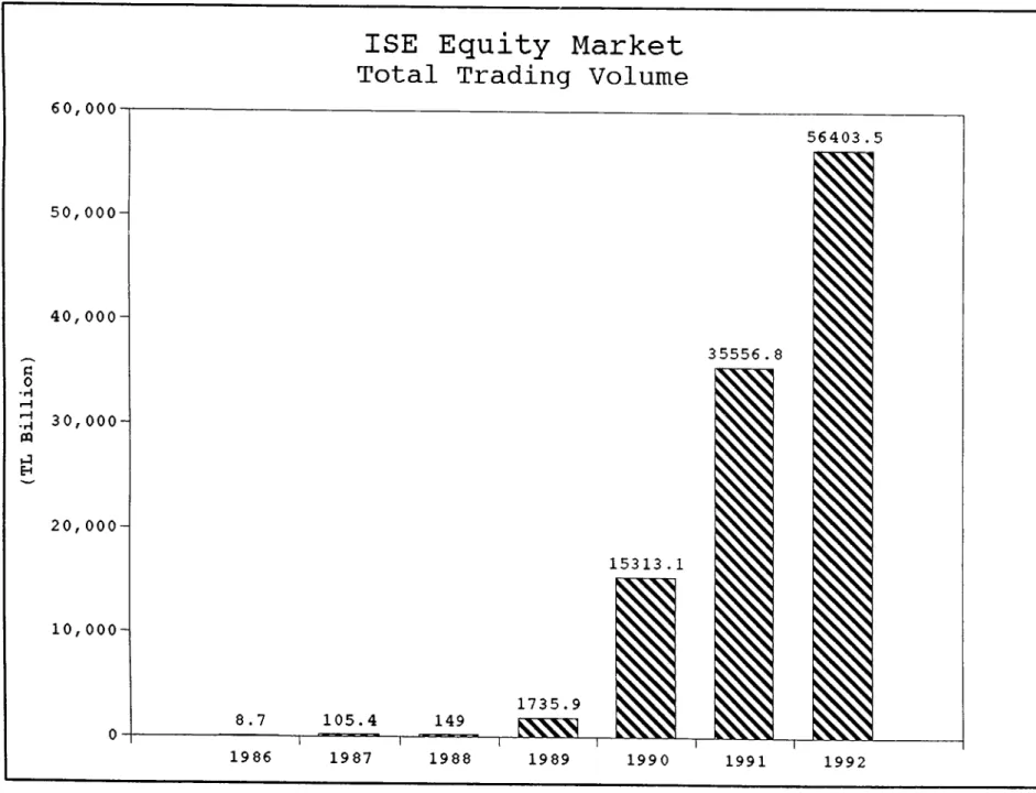
I.EMPIRICAL TESTS OF MARKET EFFICIENCY-THE CASE FOR TURKEY The Istanbul Securities Exchange (ISE) has started its operations on January 1986. For the first three years ISE could be considered as very thin(8.7 Billion TL trading volume on 1986), market showed an enormous expansion and reached to 56,403 Billion TL trading volume by the end of 1 992 (Table 9). Number of shares traded in 1986 was 3.3 million reached to 10,296
million on December,1992 (Table 9). The most important mission of stock exchange, market capitalization, increased from 709 Billion TL on 1986 to 84,809 Billion TL on 1992 (Table 8). It is obvious that the market is not thin as it has started. The development of trading volume can be seen on Table 9, but these figures does not make ISE a developed market. The trading volume should be high enough to enable any individual investor to buy or sell large amount of securities in a very short term without much affecting prices, which also is not the case in ISE in today's trading volume.
The Istanbul Stock Exchange (ISE) has been computing and publicizing a stock price index (ISE Index) as a comprehensive measure of the market's trend since January 1986 (Figure 1). The basic formula for calculating the Istanbul Stock Exchange Index is as follows : 75 It = ill 75 i = 1 >i,t * ( ) *
100
where. p . * I/O ( N ■'■ ^^1 , 0 * W ·1 , 0Pj _ = Base period price of i^^ stock 1 f CJ
Nj = Base period total no. of shares of i^^^ stock
± f U
Wj _ = The portion of i^I* stock open to public in base period
I/O
i/1 = Price of i^I* stock at period t
N± j i- = Total no. of shares of i j th stock at period t f L
W.: „ = The portion of i^^ stock open to public in period t± f U
3: [13] ISE Bulletin
So, is an indicator of the change in total market value of a common stock relative to the base period value. This index is a measure of value for an equally weighted portfolio of 75 stocks formed as the base period. The base period value of each stock is taken as a weighted average of January 1986 prices of that stock. Stock splits are also accounted for by this formula.
Some empirical studies on Forms of Efficiency were studied by Alparslan, Basel and Cadirci.
In the study carried out by Alparslan [1], the weak form efficiency tests were applied to the ISE adjusted price data. Statistical tests of independence (autocorrelation and run tests) and tests of trading rules (filter rules) have been used in these tests.
Although the runs and autocorrelation tests could not refute the weak form efficiency, the results of the filter tests revealed that an investor could have beaten the market for some stocks. Due to the large discrepancies between the buy and hold filter returns, Alparslan supports the views which are against the efficiency os Istanbul Stock Exchange.
Basel [4] investigated the distributional and time series behaviour of common stock returns in ISE for the period 1986- 1988. The study shows that published past price information can not be used to obtain better forecasts of future prices. Although, this observation is in line with the random walk behaviour the test of variance-time function indicate significant long term dependence for most of the stocks which is against weak form efficiency.
Cadirci [5] analyzed market adjustment to the release of stock dividend/right offering information (semi-strong form of efficiency) for the stocks listed in ISE for the period 1 986- 1989. Results of the study indicated that the adjustment process was slow and positive cumulative average abnormal returns are observed after the event date which leads to the rejection of market efficiency in the semi-strong sense and possibility of an above normal profit.
III. DATA AND METHODOLOGY
A. THE DATA
This study uses daily values of the Istanbul Stock Exchange Index from January 4, 1988 to December 31, 1992.
The ISE Index is used as a proxy for the realized rate of return on the market. This index is weighted by market value so price trends in the market is reflected through variations in the market value. The basic formula^ for calculating the index is as follows :
Sum of Market Values of the Portion of Constituent Companies' Market Open to the Public
--- -k Base Number Total Market Value of the Companies in the Base Period
Using each day's closing price, a return as the percentage change in the value of the index from the previous day was computed. The formula used for calculating daily percentage returns is as follows : Pl· - Pi Rt Rt = t-1 where t-1 ^t-1
percentage return for day t, index value for day t,
index value for day t-1 .
4 : Istanbul Stock Exchange Bulletin, June 1992
5 : Except Barone[3] all authors used percentage return method for calculating daily returns. Barone used a continuously compounded rate of change of the stock index which is calculated as R^=ln(P^/P^_-j).
During the entire sample period the trading days returns before and after a holiday were excluded from the data for preventing the distortion of holiday effect. So return values corresponding to 1223 trading days in the sample period were reduced to 1127 return values^.
The data were divided into two subsets : Period 1 covers from January 4,1988 to October 5,1990 and Period 2 covers from October 8,1990 to December 12,1992. This division was made because settlement day for the exchange was decreased from
2
days to1
.B. METHODOLOGY
1.TESTS OF THE DAY OF THE WEEK EFFECT
n
To test the day of the week effect the following model was used :
^t= ^
1^1
®2°2
^4^4 ^ ^ ^t where: the return of index,
u.(- : an error term assumed to be normally distributed with zero mean and finite variance,
D-^ : a dummy variable for Monday (i.e. D^ = l if observation falls on a Monday and 0 otherwise),
D
2
: a dummy variable for Tuesday (i.e. observation falls on a Tuesday and 0 otherwise).6
.· All analysis with the original data was also done.1 : Barone[3], Solnik and Bousquet[21], Connoly[8]. All authors used the same methodology to analyze day of the week effect.
The coefficients of the equation are mean returns from Monday through Friday. The regresión was run to find out whether daily returns could explain market return or not. The null hypothesis is :
Hq ■ ai =a9=a^=a/i =ac; =
0
which indicates that mean of return values for days of the week are zero,hence no day of the week effect. The null hypothesis is rejected if the F-statistic of the test is larger than corresponding f value of specific significance level and degree of freedom.
2. TESTS OF THE WEEKEND EFFECT O
The following regression® was run to test of the weekend effect;
R|-= a-j + a
2D
2+ ^3^3
^
41*4^5^5 ^ '^t
where
R
4
- : the return of index,an error term assumed to be normally distributed with zero mean and finite variance,
a dummy variable for Tuesday (i.e. D
2=1
if observation falls on a Tuesday and 0 otherwise),D
3
; a dummy variable for Wednesday (i.e.03=1
if observation falls on a Wednesday and 0 otherwise),a·^ : mean return of Monday.
8 : Barone[3] used this regression to analyze mean differences between Monday and other days of the week. Other authors used mean difference tests (t test) between Monday and each other days of the week.
^t ^t
Do
The coefficients of the equation are differences between mean returns of Monday and other days of the week. The regresión were run for the mean difference test. The null hypothesis is :
H0 a
2
-a3
-a4
-a5 - 0
which indicates that differences between mean of return values for days of the week and Monday mean value are zero,hence no weekend effect.
Since Monday average return values do not significntly differ from zero applying above methodology to find a result of existence of weekend effect do not bring a feasible solution. To verify a possible weekend effect which is mostly related to settlement procedure in the market, the above test was applied to Tuesday. That is a difference between mean return of Tuesday and mean return of other days was analyzed.
3.TESTS OF THE MONTHLY EFFECTS
To test for monthly effects the same approach as in day of the week effect is used and following regression model^ was run :
Rf= a-|D-| + a2D2 + a3D3 + a^D^ + a^D^ + agDg + a^Dy + agDg +
agDg + a-|QD-,Q + a-|-|D-|-, + a^2^l2 ^t where
: the return of index,
u^ : an error term assumed to be normally distributed with zero mean and finite variance,
9 ; Barone [4] used regression to find monthly effects in Italian stock market.
D
D-, : a dummy variable for January (i.e. D^=1 if observation falls on a January and 0 otherwise),
: a dummy variable for February (i.e. Ü
2=1
if observation falls on a February and 0 otherwise).The coefficients of the equation are mean returns from January through December. The regresión was run to find out whether daily returns of specific months could explain market return or not. The null hypothesis for this test is :
H0 ai -a
2
-a3
-a4
-a5
-ag-a7
-ag-a9
-a-| Q-a-, -a-| 2~0which indicates that mean of return values for months of the year are zero,hence no turn of the year effect.
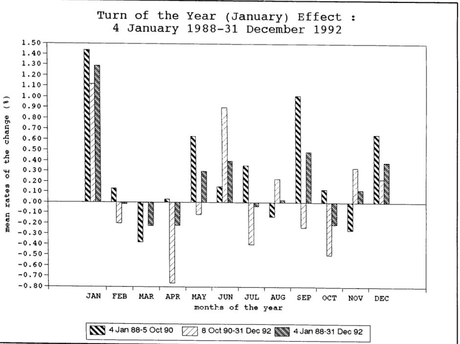
4. TESTS OF THE TURN OF THE YEAR (JANUARY) EFFECT
To make a turn of the year (January) Effect test the
1
0
following regression was run :
R^= a-| + a2D2 + ^3^ 3 ^ 4 ^ 4 "*■ ^ 5 ^ 5 a^D^ + aoDp +
igug
1
- d-| qD-| q + a-|^ l^-| -| where^
6^6
17
U7
^8^8
aoDa + a-| qD-| Q + a-|-]D-|-| + a-|2
D-]2
+Ri U4
D-the return of index,
an error term assumed to be normally distributed with zero mean and finite variance,
a dummy variable for February (i.e. D
2=1
if observation falls on a February and 0 otherwise),a dummy variable for March (i.e. 0^=1 if observation falls on a Wednesday and 0 otherwise).
10 : Barone[3] used this regression to analyze mean differences between January and other months of the year.
a-| : mean return of January.
The coefficients of the equation are differences between mean returns of January and other months of the year. The regresión was run for the mean difference test. The null hypothesis is :
H
q: a2=a3=a4=a5=a0=aY=ag=ag=a-| Q=a-| 1 =a·^ 2=0
which indicates that differences between mean of return values for months of the year and mean values of January are zero, hence no January effect.
Table 1 reports the sample return and standard deviation of days of the week. When two-tailed t—tests applied to day return values it is found that for the entire period the mean returns of Friday and Wednesday are significantly different from zero and positive.
All return values for period 1 (Table 1 ) are not different from zero which is a sign of efficiency of market. This finding is also supported by the results found in regression analysis. F-value of regression analysis for period 1 (1.55-Table 2) do not rejects the null hypothesis of equality of mean return values of days of the week.
For period 2, significant negative Tuesday return and positive Friday, Wednesday returns were found when two-tailed t- test was applied to the day returns. The F-value of regression for this period was
2 . 2 2
which rejects the null hypothesis of equality of regression coefficients. That is day of the week effect was found for Period 2.The differences of results between periods of t-tests of day returns and regression analysis about day of the week effect are as follows :
- Mean of Monday return values changes from positive in Period 1 to negative in Period 2 (both values are not significant),
-Mean of Tuesday return values changes from positive in Period 1 to negative in Period 2 (negative value is significant),
PART IV. FINDINGS
- For the Period 1 the null hypothesis of equality of regression coefficients was not rejected, where it is rejected for Period 2.
- Tuesday is the only significant contributor to the market return in regression analysis with (t value 2.25) for Period 2.
For the entire period day of the week effect was not found but F value has a significancy of 10%. The only significant contributor in the regression model for the entire period was Friday returns.
The weekend effect by definition is a return pattern occured due to positive Friday returns and negative Monday returns. But Turkish market shows a positive Monday return on Period 1 and negative Monday return Period 2 and both numbers are not significant. The results of weekend effect analysis were given on Table 3. The regression was run to find the existence of differences between Monday returns and returns of other days of the week. For the first period null hypothesis was not rejected meaning that Monday mean returns were not different than mean of other days. For the second period the null hypothesis was rejected. But this finding might not bring a result of existence of weekend effect due to the fact that Monday returns, themselves, are first not negative for Period 1 and secondly not statistically different from zero.
For the above reason and having a significant negative Tuesday return on Period 2, a further analysis of weekend effect was performed between Tuesday returns and other days for a longer weekend. Results of this analysis were given on Table 7.
For Period 2, F value rejects the null hypothesis with a significancy of 2.25%, meaning a weekend effect between Friday and Tuesday.
Therefore for the second period the inefficiency of market were being obvious due to the existence of return patterns of day of the week and weekend. Both effects are closely related to negative Tuesdays and positive Fridays. The market was efficient in the first period but findings originating from second period more likely explain the real structure of the market because in the first period the ISE was very thin, there are few participants {individual investors, corporates) in the market and market capitalization and trade volume was very low (Figure
10
-1 1
).The sample return and standard deviation for returns of months of the year are reported in Table 4. The mean return for January is positive and significant at the 1% level on first period and entire period. Mean returns on September for first period and on June for second period is positive at the 5% level.
Tests of the regression equation about month effect are reported in Table 5. For the first period the F-statistic(1.96) rejects the null hypothesis. For the second period the F- statistic do not reject the null hypothesis. January and September contributes significant information to the model for first period. The F-statistic for the entire sample period rejects the null hypothesis which means that there exists a return pattern proving market's inefficiency in monthwise.The
key month contributing significant information on market return is January. January returns are always significant in the model. In period 2 null hypothesis of equality of monthly returns other than January, was not rejected (Table
6
-F value 1.18). For the entire period null hypothesis is rejected, that is there was significant difference between returns of January and returns of other months.Major differences between periods of results of t-tests of month returns and regression analysis to find monthly effect-
January effect are as follows :
- Mean of January return values are significantly different from zero in the first and entire period but not in Period 2,
- 1.7% significant positive September return values in Period 1 changes to negative in Period 2 (negative value is insignificant),
- For the Period 1 the null hypothesis of equality of regression coefficients was rejected, where it is not rejected for Period 2.
The data were reduced by exclusion of pre and post holiday returns from the data. To check whether this exclusion affects the results of analysis, all analysis were also done with original data but no different findings listed above was observed with these analysis.
The weak form efficiency of a market requires that "changes in stock prices will be random therefore there should not be any consistent return patterns in security returns"[Radcliffe (20)]. In this study weak form efficiency of the Turkish Stock Market is tested by investigating the patterns observed in other stock market's of the world. Specifically, Day of the Week, Weekend, Month of the Year and Turn of the Year( January ) Effects were analyzed. Data set divided into two parts with the underlying property of settlement duration change. The results of 1990-1992 period focused more since it reflects market more with its higher trading volume and capitalization numbers than 1988-1990 period.
Results of the analysis about day of the week effect shows that Turkish Stock Market changes its property of being efficient as time goes. Although day of the week effect was not found for entire sample period, 1990-1992 period shows a significant day of the week effect. A significant positive Friday return was found similar to other stock markets in the world. Another similarity is the negative Tuesday return in the 1990-1992 period. Major differences between findings of two periods like changing of Monday average returns from positive to negative and Tuesday's changing from positive to negative supported the conclusion of market's trend of being inefficient.
The positive Friday return and negative Monday return creates so called weekend effect. Turkish market also shows
PART V. DISCUSSIONS AND CONCLUSIONS
weekend effect in the 1990-1992 period but this finding may be misleading. Friday returns are significantly positive for both periods but Monday returns are negative in the 1990-1992 period and it is not significant. This finding focused the analysis of weekend effect to test Tuesday returns for a longer weekend between Friday and Tuesday. Results shows a significant difference between Tuesday returns and returns of other days of the week.
A scenario about using settlement to earn abnormal returns like buying stocks on Friday and selling on Monday brings expectation of Tuesday's positive return. But data shows that Tuesday returns are significantly negative for the second period so settlement is not a complete explanation for weekend effect to occur.
Another reason for the weekend effect to occur is announcement of bad news about firms at weekends. Firms may delay such announcements until the weekend for the fear of panic selling, so allow more time for the information to be digested. This reason may be a explanation of weekend effect in the Turkish Market but will be a subject of another study. With the above findings it may be concluded that market with a positive return on Fridays (buyers in the market) shows negative returns on Monday-Tuesday and adjust itself on Wednesdays. Thursday shows a little positive yield and again a positive return on Friday.
The most significant result of this study is strong turn of the year effect. The most commonly cited reason for the January
Effect is tax-loss selling which is investor's wishing of reducing taxes by realizing capital losses at the end of the year and buying the stocks again on January. But the tax-loss hypothesis does not seem fully satisfactory. First, there is little evidence that selling pressure near year-end is strong and secondly it is not clear for the rational investors to wait the new year for reinvesting.
Another rationale for the January effect is year-end "window-dressing". In this view some portfolio and fund managers dump embrassing stocks at year-end to avoid their appearance on the annual report. This rationale is not suitable for the Turkish market because there are no professional portfolio managers in the market and most of the fund managers prefer to use T-bills of low-risk high return in their funds.
The broad cycle (Friday-Tuesday) defined above will be an sign for the speculators to earn abnormal returns but when transaction costs are taken into account, the probability that arbitrage profits are available from trading strategies oriented from above cycle seems very small. Using the result of a significant positive January return will also be an implication of this study for the investors to form a trading strategy.
Since this study is open to public, every individual investor and corporates may use the findings of this study. People try to sell on Fridays which will lower Friday returns thus market gains efficiency. That is since prices will tend to reflect all known information market become more efficient and this will be the most crucial implication of this study.
There are some shortcomings of this study which may light the findings of the study more if covered on further researchs. One shortcoming of the analysis was shortness of analysis period when compared with the periods of studies throughout the world. Results may be more satisfactory if same analysis performed for a longer period. Weekend effect under the reason of bad news releases on weekends and the effect of US and European Market Weekend Effects on Turkish Market Weekend anomaly may be studied to obtain a satisfactory explanation. Also Monday return can be accepted as a 3 calendar day return and weekend effect test can be studied accordingly.
The index announced by the Istanbul Stock Exchange is taken as a measure of market return. But Istanbul Stock Exchange changed the structure of the index at 1990. The value weighted composite index including 75 companies quoted in the market are being used through that date. Since market capitalization is still low, a drastic movement in a specific stock which has a high weight in the index formula may change the index through the side it performs although market has not moved in that way. So a better further study may be done by investigating the calendar anomalies on certain stocks (i.e. most frequently traded 30 stocks).
[1] Alparslan, S., M. (1989), "Tests of Weak Form Efficiency in Istanbul Stock Exchange", Thesis submitted to the Department of Management and the Graduate School of Business Administration of Bilkent University.
[2] Ariel, R. (1990) "High Stock Returns Before Holidays : Existence and Evidence on Possible Causes", The Journal of Finance, Vol XLV, p p . 1611-1526.
[3] Barone, E. (1990) "The Italian Stock Market-Efficiency and Calendar Anomalies", Journal of Banking and Finance, Vol 14,
pp. 483-509.
[4] Basel, E. (1989), "The Behaviour of Stock Rteurns in Turkey : 1986-1988", Thesis submitted to the Department of Management and the Graduate School of Business Administration of Bilkent University.
[5] Cadirci, B. (1990), "The Adjustment of Security Prices to the Release of Stock Dividend/Rights Offering Information", Thesis submitted to the Department of Management and the Graduate School of Business Administration of Bilkent University.
[5] Capital Market Board Monthly Bulletin, December 1992.
[7] Condonyanni, L.,
0
'Hanlon J. and Ward, C. W. R. "Day of the Week Effects on Stock Returns : International Evidence",Journal of Business Finance and Accounting, Vol 14, pp. 159— 175.REFERENCES
[
8
] Connoly, R. (1989) "An Examination of the Robustness of the Weekend Effect", Journal of Financial and Quantitative Analysis, Vol 4, pp. 132-168.[9] Fama, E. F. (1970) "Efficient Capital Markets : A Review of the Theory and Emprical Work",Journal of Finance, Vol 25,
pp. 383-417.
[10] French, R. K. (1980) "Stock Returns and The Weekend Effeet",Journal of Financial Economics, Vol
8
, p p . 55-69.[11] Gibbons, M. and HESS, P. (1981) "Day of Week Effects and Asset Returns", Journal of Business, Vol 54, pp. 483-509.
[12] Istanbul Stock Exchange Monthly Bulletins (1992).
[13] ISE Composite Index and Sub-Indices, ISE Publications No :2. [14] Jacobs, B. and Levy, K. (1988) "Calendar Anomalies : Abnormal Returns At Calendar Turning Points", Financial Analyst Journal, p p . 28-39.
[15] Jaffe, J. and Westerfield, R. (1985) "The Weekend Effect in Common Stock Returns", The Journal of Finance, Vol 11, No 2, pp. 433-455.
[16] Jaffe, J. and Westerfield, R. (1985) "Patterns in Japanese Common Stock Returns : Day of the Week and Turn of the Year Effects", Journal of Financial and Quantitative Analysis, Vol 20, pp. 261-272.
[17] Keane, M. S. (1985) Stock Market Efficiency Theory, Guidance, Implications, London : Philip Allan Publishers Ltd.
[18] Keim, B. and Stambaugh, R. (1984) "A Further Investigation of the Weekend Effect in Stock Markets", The Journal of Finance, Vol 39, No 3, pp. 819-840.
[19] Kendall, M. (1953) "The Analysis of Economic Time Series. Part 1 : Prices",Journal of Royal Statistical Society, Vol 95, pp. 11-25.
[20] Radcliffe, R. (1989) "Investment Concepts Analysis Strategy", 3rd Edition.
[21] Solnik, E. and Bousquet, L. (1990) "Day of the Week Effect on Paris Bourse", Journal of Banking and Finance, Vol 14,
pp. 461-458.
[22] Van Horne, J. C. (1986), Financial Management and Policy, New Jersey : Prentice-Hall.
APPENDICES
MEAN, STANDARD DEVIATIONS AND T VALUES OF DAILY RETURNS
TABLE 1
Period Statistic Monday Tuesday Wednesday Thursday Friday
04.01.88-05.10.90 Mean 0.461 0.452 0.346
0.021
0.257 Std.d e v . 3.500 3.251 3.196 2.676 2.512 N o .o b s . 1 1 71
20
11
91
20
1
22
t value * 1 . 43 1 . 52 1.18 0.09 1.13 08.10.90-31.12.92 Mean -0.057 -0.685 0.466 0.009 0.591 Std.dev. 3.983 2.958 2.352 3.326 2.808 N o .obs.1
061
06 106 1 07 1 04 t value * -0.15 -2.39 2.04 0.03 2.15 04.01.88-31.12.92 Mean 0.215 -0.081 0.402 0.016 0.411 Std.dev. 3.737 3.162 2.824 2.993 2.652 N o .obs. 223 226 225 227 226 t value *0 . 8 6
-0.39 2.14 0.08 2.33* The underlined figures are significantly different from zero at the 5% level.
T A B L E 2
TEST OF THE DAY OF THE WEEK EFFECT *
Statistic Model Monday Tuesday Wednesday Thursday____ Friday 04.01 .88-05.1 0.90 08.10.90-31.12.92 04.01.88-31.12.92 Coefficient t value ** deg. of fr. f value *** Coefficient t value ** deg. of fr. f value *** Coefficient t value ** deg. of fr. f value *** 593 1 . 55 524 2.22
1
1
22
1
.81 0.461 1 . 64 -0.057 -0.19 0.215 1 .04 0.452 1 . 63 -0.685 -2.25 -0.081 -0.40 0.346 1 .24 0.466 1 .53 0.402 1 .950.021
0.08 0.009 0.03 0.016 0.08 ** 'k'ki< 0.257 0.93 0.591 1.92 **** 0.411 2.00 Rt=b1 D1 -i-b2D2-t-b3D3-i-b4D4-i-b5D5-i-ut Null Hypothesis H O :b1=b2=b3=b4=b5=0The underlined figures are significantly different from zero at the
5
% level, meaning contributing significant information to the model in presence of other variablesfigures are significantly different from zero at the
5
% level, which indicates **** of null hypothesis. Market return can be explained by daily returns,significant %5.o4
T A B L E 3
TEST OF THE WEEKEND EFFECT (MONDAY) *
Period Statistic Model
Tuesday Wednesday Thursday Friday 04.01.88-05.10.90 Coefficient t value ** deg. of fr. f value *** 593 0.42 -0.009 -
0 . 0 2
-0.115 -0.29 -0.440 -1.11
-0.204 -0.52 08.10.90-31.12.92 Coefficient t value ** deg. of fr. f value *** 524 2.73 -0.629 -1 . 46 0.5221
.21
0.066 0.15 0.647 1 .50 04.01.88-31.12.92 Coefficient t value ** deg. of fr. f value ***1
1.171
22
-0.297-1
.02
0.187 0.64 -0.199 -0 . 6 8
0.195 0.67Test of difference between mean returns of Monday and other davs Rt=a1+b2D2+b3D3+b4D4+b5D5+ut
Null Hypothesis H O :b2=b3=b4=b5=0
The underlined figures are significantly different from zero at the
5
% level, mei *** significant information to the model in presence of other variablesr S j e c ? ? n 5 o r L f i ' h i p o t S ^ i s ! " " ^ ^ - ^ i - t e s
meaning
TABLE 4
MEAN, STANDARD DEVIATION AND T VALUES OF THE MONTHS OF THE YEAR *
Period Statistic Jan Feb Mar Apr May Jun
Jul Aug Sep Oct Nov Dec 04.01.88-05.10.90 08.10.90-31.12.92 04.01.88-31.12.92 Mean Std.dev. N o .o b s . t value *'■' Mean Std.dev. N o .o b s . t value ** Mean Std.dev. N o .o b s . t value ** 1.438 0.131 -0.38 0.032 0.629 0.150 0.353 3.382 3.654 2.776 2.267 2.533 2.174
2.577
48 49 61 55 51 64 2.95 0.25 -1.06 0.10 1.77 0.55 43 0.90 -0.14 1.015 0.125 -0.26 0.647 3.776 3.102 4.279 2.850 2.335 57 45 1.121 -0.20 -0.01 -0.77 -0.12 0.903 -0.40 4.236 3.484 2.394 2.227 3.011 2.5172.355
42 40 43 25 41 1.71 -0.37 -0.02 -1.72 -0.25 32 46 2.03 -1.16 51 -0.27 0.225 3.262 41 0.44 35 39 2.47 0.20 -0.55 1.73 -0.24 -0.50 0.333 0.224 2.126 2.046 3.824 4.090 42 -0.74 52 -1 . 76 63 0.69 62 0.43 1.290 -0.02 -0.22 -0.22 0.297 0.401 -0.04 3.786 3.562 2.619 2.271 2.766 2.308 2.480 90 89 104 80 92 3.23 -0.05 -0.87 -0.86 1.03 96 89 1.70 -0.14 0.022 0.482 -0.21 0.120 0.387 3.542 2.789 3.273 3.504 3.509 92 99 97 98 101 0.06 1.72 -0.63 0.341.11
* The percentage rates of change corresponding to pre and post holidayshave been excluded.
** The underlined figures are significantly different from zero at the 5% level.
T A B L E 5
TEST OF THE MONTH OF THE YEAR EFFECT *
Period Statistic Model Jan Feb Mar
Apr May Jun Jul Aug Sep Oct Dec
04.01.88-05.10.90 Coefficient t value ** deg. of fr. f value *** 586 1 .96 1.438 0.131 3.29 0.30 -0.38 0.032 -0.98 0.08 0.629 1 . 49 0.150 0.353 0.40 0.77 -0.14 -0.33 1.015 2.54 0.125 0.28 -0.26 -0.52 0.647 1 .34 08.10.90-31.12.92 Coefficient t value ** deg. of fr. f value *** 517 1 .09
1.121
-0 . 2 0
2.31 -0.40 -0.01 -0.77 -0.01
-1 . 2 2
-0 . 1 2
-0.24 0.903 -0.40 1.62 -0.87 0.225 0.46 -0.24 -1.14 -0.50 0.84 0.333 0.56 0.224 0.43 04.01.88-31.12.92 Coefficient t value ** deg. of fr. f value *** 1115 1 .98 1 .290 -0 . 0 2
3.97 -0.06 -0 . 2 2
-0 . 2 2
-0.74 -0.63 0.297 0.92 0.401 -0.04 1.28 -0.11
0 . 0 2 2
0.07 0.482 1 .56 -0.21
-0.670 . 1 2 0
0.39 0.3871
.26 * Rt-bl D1+b2D2+b3D3+b4D4+b5D5+b6D6+b7D7+b8D8+b9D9+b10D10+b1lDl1+b12Dl2+ut Null Hypothesis H O :b1=b2=b3=b4=b5=b6=b7=b8=b9=b10=b11=b1 2 = 0** The underlined figures are significantly different from zero at the
5
% level, meaning *** significant information to the model in presence of other variables.figures are significantly different from zero at the