Experimental results and bifurcation analysis on scaled feedback control for subsonic cavity flows

Experimental

Results and

Bifurcation

Analysis

on

Scaled

Feedback

Control for Subsonic

Cavity

Flows

X. Yuan, E.

Caraballo,

M.

Debiasi,

J.

Little,

A.

Serrani*,

H.

Ozbay

and

M.

Samimy

Abstract-In this paper, we present the latest results of fromDepartmentsof Mechanical

Engineering

and Electrical ourongoing research activities in thedevelopmentof reduced- and Computer Engineering at OSU, Air Force Research order models based feedback control of subsoniccavityflows.

Laboratory,

and NASA

Glenn,

possesses synergistic capa-The model wasdevelopedusingtheProperOrthogonalDecom- ... . ' . '

position of Particle ImageVelocimetry images in conjunction

bilities

in all ofthe

required

multdisciplinary

areas

of flow with the Galerkin projection of the Navier-Stokes equations simulation, reduced order modeling, controller design, and onto theresulting spatial eigenfunctions. Stochastic Estimation

experimental

integration

and

implementation

of the compo-method was used to obtainthe state estimation of the Galerkin nents along with actuators and sensors, . The ultimate goal system from real time surface pressure measurements. A istoenable theuseof

closed-loop aerodynamic

flow control

linear-quadratic optimal controller was designed to reduce to

enabl

the

ueof

osed-loopuaeronam

iclw cnt

cavity flow resonance and tested in the experiments. Real- to control theflow o n e vehicles and

timeimplementationshows asignificantreduction of the sound ultimately to control the motion of the vehicles themselves. pressure level withinthecavity,with a remarkable attenuation The initial

application

chosenas a benchmark

problem

for of the resonant tone and a redistribution of the energy into study is closed-loop control of the acousticresonance of a various modes with lower energy levels. A mathematical flow over a shallow cavity

[14], [15],

[18].

The objective of analysis of the performance of the LQ control, in agreement the

current

work isto

provide

a

comprehensive

overview of

with theexperimental results, is presented and discussed. the ctivit of

to

grou ndea feedbacko ntrol

the activity of the group on modeling and feedback control

I. INTRODUCTION design, including apresentationof thespecific experimental

setup andamathematical discussion of the results obtained

The generation of tones by flow past an open cavity ineprm tadsmuto.

is a well known phenomenon which affects landing gear The paper is organized as follows: the experimental and weapons bays on aircraft. This flow is characterized

apparau

is

described

in S

onlIIs

Se

expediscusse

bya complex feedback process that leads to self-sustained

reduced-oderimodein

techn

of

caity

flo

dics.

oscillations referred to as Rossiter [13] mechanism: small

rollerdes

rel teimpementation

danalis

disturbances are amplified by the

cavity

shear

layer,

and

onthe

rear

te

inpSection

I

olloedib

nd

produce acoustic waves when

they

impinge

on the down-

concluding

remarks

in Section

V.

stream corner of the cavity; these acoustic waves then

propagate upstream and excite further instabilities in the II. EXPERIMENTAL APPARATUS

shear layer, leading to

self-forcing.

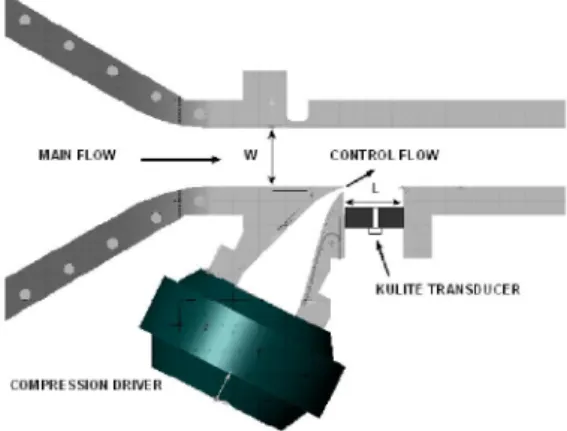
The sound pressure In this section we outline the

experimental

setup de-levels of thetones canbeashighas 160dB,whichcan cause scribed in more detail in Debiasi and Samimy [6]. The core structural damage in air vehicles. While

passive

and open- ofthe

experimental

setupconsists ofan

optically accessible,

loop active controlmethodologieswere

extensively applied

blow-down type wind tunnel with a test section of width for the suppression of cavity flow tones in past

studies,

W= height H = 50.8 mm. A cavity that spans the entire feedback control has only

recently

been

employed

to this width of the test section is recessed in the floor with a

problem (see Cattafesta et al. [2] for a recent

review)

and depth D = 12.7 mm and length L = 50.8 mm for an the effects of the closed-loop

dynamic

control on the flow aspect ratio

L/D

4. For control the

cavity shear-layer

dynamics are not well understood yet. receptivity region is forced by a 2-D synthetic-jet type The flow controlteam atthe Ohio State

University

(OSU)

actuator issuing at 30 degrees relative to the main flow Collaborative Center of Control Science

(CCCS)

is

working

from a 1 mm slot embedded in the cavity leading edge and

to develop tools and methodologies for closed-loop aero- spanning the width of the cavity, see Fig. 1. A Selenium dynamic flow control. The team, composed of researchers D3300Ti compression driver provides the mechanical

os-This work issupported in part by AFOSR and AFRL/VA through the ciltin neesr'ocet h zr e as ozr

Collaborative Center of Control Science (Contract F33615-01-2-3 154). net momentum flow for actuation. The actuator signals

X. Yuan and A. Serrani are with the Department of Electrical & are produced by either a BK Precision

3011lA

function ComputerEngineering, the Ohio State University, Columbus, OH, 43210 geraofropnlpfrcgorbadSAE10DP

E. Caraballo, M. Debiasi, J. Little and M. Samimy are with Gas Dy- geeao fo opnlo ocn rb SAE10S

namics and Turbulence Laboratory, Mechanical Engineering Department, control board In closed-loop studies and are amplified by the Ohio State University, Columbus, OH 45235-7531. a Crown D-150A amplifier. The pressure fluctuations are H. Ozbay is with the Department of Electrical & Electronics Engineer- measured by Kulite dynamic pressure transducers placed

ing, Bilkent University, Ankara, TR-06533, Turkey; on leave from The indfentlciosnthtsteto.AdPCE10

OhioState University. 1 1frn oa1n ntets ehn SAE10

computer is used to simultaneously acquire the pressure explicit expression of the control effect inthe equations to signals at 50 kHz through 16-bit channels and manipulates facilitate the design of the feedback control law. Meanwhile them to produce the desired control signal from a 14- stochastic estimation is usedto estimate the states based on bit output channel. Each recording is band-pass filtered real time surface pressure measurements.

between 800 and 10,000 Hz to remove spurious frequency

components. The "snapshots" of the flow field, required for A. POD Method

The POD method was introduced to the fluid dynamics

community by Lumley [12] as a way to extract large-scale structures in a turbulent flow. The general idea is to

decompose

the flow field into a set of

orthogonal spatial

basis that contains the most dominant characteristics of

:AINFLOW

1ONTROL

W FLOW the flow. More details of the fundamentals of this method can be found in Holmes et al.

[10].

The POD

approach

under

investigation

is the

snapshot

method

[16],

which is

K

_ITE

TRANSDUCER more suitable for

highly spatially

resolved data sets that

| 11 iw , ~~~~~~KULITETRANSDUiCER

can be obtained

using

numerical simulations or advanced laser-based flow

diagnostics. Applying

the POD method COMPRESSION DRIVE t _ _ results in a

temporal-spatial decomposition

of a flow

variable (e.g. the streamwise velocity u(x, t)) as:

N

Fig. 1. Cutoutof the wind tunnelshowingtheconverging nozzle,thetest

u(x,

t)

E

ai(t)

oi(x),

(1)

section, the cavity, the actuatorcoupling, and the placement of a Kulite transducer in thecavityfloor.

where i

(x)

are spatial modes that capture the coherent the

development

of the low dimensional

model,

are

acquired

structures and time coefficients ai

(t)

are function of time and

processed using

a LaVision Inc. PIV

system.

Details

only

and

represent

the time evolution of the

corresponding

> . . . .

~~~~~~~~~~~coherent

structures. ofthe PIV system, procedure, andresults are presented in

[ 1]. The main flow is seeded with Di-Ethyl-Hexyl-Sebacat B Galerkin

Projection

(DEHS) particles by using a 4-jet atomizer upstream of the

stagnation chamber. A dual-head Spectra Physics PIV-400 The Galerkin projection method was used to acquire a Nd:YAG laser operating at the 2nd harmonic (532 nm) is low dimensional model of the cavity flow in the form of used inconjunctionwith sphericaland cylindrical lenses to a set of ODE's for the time coefficients a(t). The method form a thin(

1mm),

vertical sheetspanning the streamwise relies on the projection of the governing equations of the direction of the cavity at the middle of test section width.

flow,

the

compressible

Navier-Stokes in this case, onto the

Two CCD cameras (2K by 2K) with maximum acquisition POD

spatial

basis derived by POD decomposition. Refer

frequency of 15 Hz capture the images when the laser is to

[3], [15]

for a detailed

description

of the derivation of fired. Dedicated software is used to process the images and this model. It's worth to notice that a standard Galerkin obtain the velocity flow field information. This setup gave

projection

results in an ODE model with external control

avelocity vectorgridof 128by 128 overthe measurement effect

implicitly expressed

in the

model,

which is not useful domain of 50.8mmwhich translates to eachvelocity vector for controller

design.

In orderto derive amodel where the

being separated by approximately 0.4 mm. In the initial control

input

appears

explicitly

in the equations, a control

phase of the experiments only 2 velocity components are

separation

methodwas

incorporated

into the Galerkin

pro-obtained. jection

procedure.

The main idea of the control separation

is to separate the sub-domain of space where the external

III. REDUCED-ORDER MODELING control input is introduced into the flow field from the rest

Reduced-order models of the flow werederived from PIV of the field, as detailed in Efe and Ozbay [8], [9], which snapshots and surface pressure measurements of the cavity yields a system in the following form:

flow as described in detail by the authors in previous works

[3], [4], [15]. The approach is based on the combination of

(aTH1a8

three independent tools. First, the POD method is used to a=F+ Ga + | B+| |), (2)

acquire a spatial basis of the velocity field. Then, Galerkin VaTHNa

V-projection method is applied to obtain the flow model in

the form of a set ofordinary differential equations for the where the matrices ofconstant coefficients F, G, Hi, B and POD temporal coefficients (states of the system model). In

if,

i =1, ,N, are obtained from the Galerkin projection, the process of projection, the domain of control input was and

17(t)

is the control input applied at the forcing location, separated from the rest ofthe flow field which results in a detailed in Yuan et al. [19].

C. Stochastic Estimation where

The Stochastic Estimation (SE) method has been used

(aT

(H1

+

H1T)1T

here to estimate the time coefficient of the Galerkin system G=G +

,B=

B +

aO.

(2) for feedback flow control. SE was originally proposed T H4

H4T)

4T

and used by Adrian [1] as a method to extract coherent 0

(

+H \

structures from a turbulent flow field. The technique es- Clearly, the modified model has an equilibrium point atthe timates flow variables at any location by using statistical origin, which is more convenient for controller design and information about the flow at a limited number oflocations. stability analysis.

Inanyrealistic setting,the real-timeexperimentaldata could

only be obtained via surface measurements (e.g. surface B Linear Quadratic State Feedback Control

pressure or surface shear stress measurements). In the A linear

approximation

of

(4)

at the

origin

is

readily

currentwork, quadratic stochastic estimationwasemployed obtained as

to estimate the time coefficients of the flow model (2) a =

Ga

+

BF.

(5)

directly from real-time measurements of surface pressures The

eigenvalues

of the

system

matrix G have been com-p

(t)

at asmall number of locations L = 6. The estimates of puted for the three cases

respectively

and show the same the time coefficients can be written in the following form:

_qualitative

X _{features (2 unstable complex conjugate}

eigen-6,i(t) CikPk(t) +DiklPk(t)1(t), k~ 1~... 6 (3 values plus 2 stable real eigenvalues) and quantitative

&a

(t) CikPk(t) + Diklpk(t)pi(t), k,1 1,

,..~

6 (3)

similarities

as well. The presence of two

unstable

complex where C D are the matrices of the estimation coefficients

conjugate eigenvalues implies,

as

expected,

that the mean

obtainedby minimizing the averagemeansquareerror flow

(corresponding

to the

equilibrium)

is an unstable

obtained by minimizing the average mean square error souinfrteGeknsyem()

between the values ofai obtained from the

snapshots

and souto fo th Gaeri sytm(

betweenthe

vstim

aludones

ofi

aobtaine

the s

napshotsmand

Controllabilityof thepairs

(G,

B) for all casesand

avail-the esimte oe atesaeim.ability of real-time state estimates of the Galerkin model

renderedbystochastic estimation (3)allow theuseof linear

IV. FEEDBACK CONTROLANDANALYSIS state-feedback controller in this study. A standard

linear-quadratic (LQ) optimal controller based on the linearized Inthis section, wepresentthedesign of the model-based

model

(5) was designed in the

form

controller, discuss the real-time implementation

results,

and interpret the results from a mathematical

perspective.

F

=-Ka

(6)

The design procedure includes equilibrium computation, and whereafter

applied

to the nonlinear Galerkin model. coordinatestransformation,linearapproximationand linear- Simulation results have shown that the LQ controller

de-quadratic state feedback control design, which is described

signed

for the linear

approximation (5)

succeeds in stabi-in[4], [19] inmoredetail. Three reduced-order flow models lizing the equilibrium of the four modes nonlinear Galerkin obtained by reduced-order modeling techniques discussed system (2), as indicated in Fig. 2.

in Section III have been investigated in this work: (i) the

baseline Mach0.3flow; (ii)the baseline

flowforced

at3920 C. Real-Time Control

Implementation

Hzusingopen-loopsinusoidal excitation;

(iii) aflow

model In this part, we summarize the results obtained in the obtainedfrom POD modes derived by concatenating PIV realtime experimental implementation of the LQ feedback datasets

from

the two cases i and ii in time. The reduced- controller. It is important to point out that, to prevent order flow model for all the cases for control

design

is the damaging the actuator, the control input signal is limited

samenonlinearstate spacemodelgiven

by (2),

with N= 4, to the range

±10V.

Since the LQ control by design is to whereas the numerical values of the model parameters completely eliminate the pressurefluctuations which results

obviously varies for each flow condition. in quite large control gains, a constant saturation of the

actuator was observed during

closed-loop

experiments.

In

A. Equilibrium Analysis and Model

Simplification

order to keep the actuator below the saturation limits, a constant scaling factor

ag

> 0 was introduced into the Defining a -

a-a

as the new set of coordinates, where feedback loop. The largest feasible scaling factor has been

a0

is the equilibrium point computed for the model (2), found for all three flow models respectively as: and shifting the origin of the coordinates to the equilibrium

point corresponding to the mean flow gives a simplified

aE1

=0.265,

ag2

=0.35,

ag3

=0.5,

(7)

state space model in the new set of coordinates as and the actual control law was scaled by

ag

as: a =

Ga+. + Br + . r (4) The scaled LQ controls (8) have also been simulated on

-02X______________________--_a 0.02 tpjp 0.4 a2~~~~~~~~~ 0.01 0.6 a ~~~~~~~~~~~~~~~~~~~~~~~~~~~0.01 0.4 -0.03 0 it P. 0.002) 0.004 0.006 0.008 0.01 _{-0.4 ~~~~~~~~~~-}( _a20.140 _05"=0.002 0004 0 006 0 008 0 01 0 012 a4 0.12~~~~~~~~~~~a0.6

whr

(tepant

is. tae 0to0 0be:0(a)baselin flwmdl()cmie dfeetsalnatr(a) baselin flo 0odel0(b)combine baselin and001 04 ~~~~~~~~~~~~~~~~~~~~~~~~~~~~~~0.16 - - - ~~~~~~~~~~~~a20.082 0.6 a~~~~~~~~~~~~~~~~200 0t~~~~~~~~~~~~~~, ~~ ~ ~ ~ ~ a30.04 0.4 ~~~~~~~~~~~~~~~~~~~~~~~~~~~~0.02 -0.02 -0.04 _0. 002 0.00 .0 .0 .102 0.0-.0 .0 008 00 .1

baseline and open-loop forced flow model (forcing frequency 3920Hz). open-loop forced flow model (forcing frequency 3920Hz).

It is evident that, though the scaled LQ control for the Recall that G in (4) has 2 unstable complex conjugate given values of

ag

is not able to asymptotically stabilize the eigenvalues and 2 stable real

eigenvalues._Let

T C

2~4x4

origin of the nonlinear model (2), it nevertheless provides be a nonsingular transformation that puts G in modal form a significant reduction of the amplitude of the stable limit

cycle in all three cases. This result is in agreement with TGT-1 (1L 0 %

a mathematical analysis carried on the nonlinear finite- L2

dimensional Galerkin model (4) given in Section IV-D. L1=(5 W), L2 = (-Ai

The performance of the scaled control law (8) has been

\W

'JU/

-2

tested experimentally, for different flow conditions. Here- where

uJ

> 0,

w<

> 0, A1 > 0, and A2 > 0. Partitioning after, we present the results obtained for Mach 0.3 cavity the state vector according to the above decomposition, the flow. Specifically, we present the closed-loop sound pressure Galerkin system is written in the new coordinates as level (SPL [dB]) recorded by the sensor located at central

cavity floor with each scaled LQ controller designed on 1 = Lir1 + M1]7 +&bi(ry, ()+ 71(r1,

()F

the basis of the three flow models discussed above. The = L24+

M2F

+

b2(ij,

() +

'72(17,

()F

results for closed-loop scaled LQ control, shown in Fig.

4,

hr

show a considerable attenuation of the resonance peak, and wee T -t8 T 1/1

a redistribution of the energy into various modes, especially a<y,t2

lower frequency modes, with much lower energy level. The

scaled LQ state feedback control has also been shown to

zi(rj,

() =O(lr

2,

ll

2),

successfully reduce the dominant Rossiter peak and provide t(1 )=°|71, ll, i=1,2

good robustness when applied to off-design flowconditions 7J7 O( , 1,2

around Mach 0.3. Note that the control law F =-aKa can be expressed in

the new coordinates as

D. Mathematical Analysis of the Performance of LQ Con-F K1 K Q

trol

r=a1r-vX

In what follows, we present a simple analysis, carried out for some matrices K1 and K2. Since it has been verified that on the basis of the nonlinear Galerkin model, toexplain the the control input does not affect the location of the stable closed-loop results obtained with the LQ feedback control. eigenvalues of the open-loop matrix G, as it is typically

140 Baseline since >>»

(7,

and a e [0,1]. Letting ,= 1- 2a, one 13s 1336dB (aseline) obtains (modulo a unitary transformation)

130

125

L,-

oV1Kl

(ao

-w)

'

120-\W 11-1

116.7dB

115 and thus the spectrum of the closed-loop matrix

0- 110

105 (

L,

+

(Ii/2

-

1/2)M1Kl

0\

100o

Lqt) ( (/,2-

1/2)M2K2

L2)

90

splits into a pair ofpurely imaginary

eigenvalues

and a

85 pair ofnegative realeigenvalues when ,u=

0.

This implies

(a)

103 104 the existence ofa center manifold for the trajectories of

140 - Bsi the Galerkin system.

Specifically,

denote for the sake of

135 133.6dB - LQ(3920) simplicity

130-125

-L

(h)

=LJ1

120 L21(,u) L21'

116.3dB

m 115

i(r7,qt)

= (T71, )-

ay(T ()Krl

7

i=1,2

1110

105 and write the

closed-loop

Galerkin system as

100 95-90 rj

Lii(fi)T

+

i1(T,(,11 )

() 853 4 L21(11)T+L2( -+ 2(T1,(:P)

(b)

io3 where 140

135 - ned) |bi(r, i) O( for all ,u, 1,i2

130 and we have added a trivial dynamics for the bifurcation

125 parameter

,u.

The Center

Manifold

Theorem [5]

establishes

120 114dB the existence of an exponentially attracting submanifold

110 of the state space, which is described

by

the

graph

of

105

a smooth

mapping

= 7

(rj, u) satisfying 7(0, )

= 0,

100r

(0

w/ )(,

q =)

0,

and

95 -07

853

4L=1((,)Tj

+

q257(Tw,

wP)

+

2(TI)]

(TI, P), P)

(c) 103 frequency (Hz) 10+

for all

(rj,

,u)

in a neighborhood of

(0,

0).

This allows to

Fig. 4. Soundpressure level inclosed-loopexperimentswithLQ design reduce the analysis of the dynamics of the Galerkin system

basedonbaseline flow model (a), forced flow model (b), and combined toits restrictionontothe centermanifold, which in thegiven

flow model(c).

setof coordinates reads as

012

_ A O

-A01

+T/

K12

(,

7

(q, P),

P)A

the case for

LQ-based

design,

necessarily K2

=

[O

0]. - (i )

-(s)

+

¢2ij,7F(1,/l),L))

Therefore,theclosed-loop systemcanbe written in the form A

near-identity

transformation into

Poincare

normal form [17] yields

=(Li aMiKitj + bi(r, - a'y1(r)K1rj q5ii(r1,w(r1,,u),,u) (-a(,u)rji-b(,u)rj2)p2 °O 5)

-aM2Kij +2&~ <'2(7, ~)- a'2(rj,~)K1r.

4b2(ij,

w(ri7,

,'),

8)

=(b(,u)rj

-

a(1)172)p2

+

O(l iil

5),

An easy computation shows that the eigenvalues of

the2

matrix L1

-aM1IK1

are given by _{nates one obtains}where

po

= /+_{the system}and

a(Li)

>

0.

Using

polar

coordi-A(L1 -

aMiKi) =(1

-

2a)o-

+j

w/>2

+

4o-J2

(1 -

a),

p uo-p-

aQi)

p3 + 0(p5)

and thus

where 0

=tan-1

(r12

/r11)).

Thestructure ofthe reduced

exponentially stable equilibrium at the origin for ,u < 0, and Chris Camphouse, John Casey andKihwanKim and Cosku undergoes a Hopf-Poincare-Andropov bifurcation at ,u = 0, Kasnakoglu for fruitful and insightful discussions.

with a stable limit cycle for ,u > 0. The amplitude and

frequency of the limit cycle are given respectively by REFERENCES

[1] R. J. Adrian, "On the Role of Conditional Averages in Turbulent w_ /125*- +

b(t)AP/

Theory,"Turbulence inLiquids,SciencePress, Princeton, 1979.

a(

) - a(,u) [2] L. N. Cattafesta, D. R. Williams, C.W. Rowley and F. S. Alvi,

"Review of Active Control ofFlow-Induced Cavity Resonance",

from which, since a(,u) 0(1), it is readily seen that AIAAPaper 2003-3567, June2003.

the amplitude of the oscillation decreases as , 0+. [3] E. Caraballo, J._{SubsonicCavity Flows - Low Dimensional Modeling," AIAA Paper}Malone, M. Samimy, and J. DeBonis, "A Study of Recalling that ,u = (1 - 2a), the results of the analysis 2004-2124, June 2004.

can be summarized as follows: [4] E. Caraballo, X. Yuan, J. Little, M. Debiasi, P. Yan, A. Serrani,

J.MyattandM. Samimy,"Feedback Control ofCavityFlowUsing

1) If it iS required to seta < 0.5 to avoid saturating the ExperimentalBased Reduced Order Model," AIAA Paper 2005-5269,

actuator, theorigin of the Galerkin system can not be June2005.

stabilizedat all. [5] J. Carr,_1981. Applications of Centre

Manifold

Theory, Springer-Verlag,

2) If this is the case, the application of linear feedback [6] M. Debiasi and M. Samimy, "Logic-Based Active Control of

Sub-can still lower the amplitude of the limit cycle, but sonic Cavity-Flow Resonance",AIAAJournal, Vol. 42, No. 9, pp.

only up to the critical value imposed by the actuator _{[7] J.}1901-1909, September 2004._{Delville,L.Cordierand J. P. Bonnet, "Large-Scale-Structure}

Iden-limits. tification and Control in Turbulent Shear Flows," In Flow Control:

The experimental results seem to support the results of the_{analysis,aslinear} Fundamentals and Practice, (M. Gad-el-Hak, A. Pollard and J.

feedback is capableto attenuatethereso-

[8Bonnet),

pp. 199-273, Springer-Verlag, 1998.

analysis, as l1near feeback 1S cpable to ttenuate he reso- 8] M. 0. Efe and H. Ozbay, "Proper Orthogonal Decomposition for

nance inthe cavity to a certain extent, while complete sup- Reduced Order Modeling: 2D Heat Flow," Proc. of IEEEInt.Conf. pression seems to beunattainable with the given actuation. onControlApplications (CCA'2003), June 23-25, Istanbul, Turkey,

However, t maystil be posible to rduce the mplitude 2003a.

However, it may still be possible to reduce the amplitude [9] M.0.EfeandH.Ozbay, "Integral Action Based DirichletBoundary

of the cavity tone beyond the limit achievable using linear Control of Burgers' Equation," Proc. of IEEE Int. Conf. onControl

feedback, resorting to different control strategies (nonlinear Applications(CCA'2003),June 23-25, Istanbul, Turkey, 2003b. feedback ortime-varying feedback). In particular, a viable [10] P. Holmes, J. L. Lumley and G. Berkooz, Turbulence, Coherent

Structures, Dynamical System, and Symmetry, Cambridge University

strategy tobe pursed is to increasea(,u), shaping the center Press,Cambridge, 1996.

manifold = 7(rj, ,u) bymeans of nonlinear feedback. [11] J. Little, M. Debiasi and M. Samimy,"Flow Structure inControlled and Baseline Subsonic Cavity Flows", AIAA Paper 2006-0480, V. CONCLUSIONS AND FUTUREWORKS _[12] January 2006._{J. Lumley, "The Structure of Inhomogeneous Turbulent Flows",} The work presented anddiscussed ispartofour ongoing AtmosphericTurbulence andWavePropagation, Nauka,Moscow,pp.

research activities in the development of reduced-order _{[13] J. E.}166-176, 1967._{Rossiter, "Wind Tunnel Experiments on the Flow Over} Rect-models based feedback control of subsonic cavity flows. angular Cavities at Subsonic and Transonic Speeds", RAE Tech.

PIV data and the POD technique are used to extract the Rep. 64037, 1964and Aeronautical Research Council Reports and most energetic flow features. The Galerkin projection of _[14] Memoranda No. 3438, October 1964._{M.Samimy,M.Debiasi,E.Caraballo,H.Ozbay,M.0.Efe, X. Yuan,} the Navier-Stokes equations onto the POD modes was J. DeBonis, and J. H. Myatt,"Development of Closed-Loop Control used to derive a set of ordinary differential equations, forCavity Flows", AIAAPaper 2003-4258,June2003b.

which govern the time evolution of the modes, and to [15] M. Samimy, M. Debiasi, E. Caraballo, J. Malone, J. Little, H. Ozbay,_{M. 0. Efe, P. Yan, X. Yuan, J. DeBonis, J. H. Myatt and R. C.} use for the controllerdesign. Stochastic estimation is used Camphouse, "Exploring Strategies for Closed-Loop Cavity Flow to estimate the state of the Galerkin system from real- Control",AIAAPaper 2004-0576, January2004.

time pressure measurements. A linear-quadratic optimal [16] L. Sirovich,_Quarterlyof"Turbulence_{Applied Math,}and the_Vol.XLV,Dynamics of Coherent_{N.3,pp. 561-590,}Structures",_1987.

controller was designed and implemented to reduce cavity [17]

S.

Wiggins, Introduction to Applied Nonlinear Dynamical Systems flow resonance. A mathematical analysis was performed andChaos, Springer,2003.

to explain the closed-loop results obtained with the LQ [18] P. Yan, M._{J. M.Myatt,}Debiasi, X. Yuan, E._{andM. Samimy, "Modeling and Feedback}Caraballo, A. Serrani,_{Control for}H. Ozbay, feedback control. Notwithstanding the encouraging results Subsonic Cavity Flows: A Collaborative Approach", Proc. 44thIEEE

reported and discussed in this work, further investigation is CDC-ECC, Seville, Spain, 2005.

needed to understand how to incorporate more effectively [19] x. Yuan, E._{J. H. Myattand M.}Caraballo,_Samimy,P. Yan, H. Ozbay, A. Serrani,J. DeBonis,_{"Reduced-order Model-based Feedback} the presence of actuation inreduced-order POD models, and Controller Design for Subsonic Cavity Flows", AIAA Paper 2005-to pursue different control strategies (nonlinear feedback 0293, January, 2005.

Or time-varying feedback) to overcome the limit posed by linear feedback control.

VI. ACKNOWLEDGMENTS

The support of AFRL/VA and AFOSR under Contract

F33615-O1-2-3

154 is gratefully acknowledged. The authors would like to thank Drs. James Myatt, James DeBonis,