Design and implementation of a PC based medical image workstation

ш г к ш iiPÍíi£iií¿íiis If I re

ш ш

- v.re'reo' ijyJi^OpT/^

" é l T

DESIGN AND LMPLEMENTATION OF A PC BASED

MEDICAL IMAGE WORKSTATION

A THESIS

SUBM ITTED TO THE DEPARTMENT OF ELECTRICAL AND

ELECTRONICS ENGINEERING

AND THE INSTITUTE OF ENGINEERING AND SCIENCES

OF BILKENT UNIVERSITY

IN PARTIAL FULFILLMENT OF THE REQUIREMENTS

FOR THE DEGREE OF MASTER OF SCIENCE

By

Omer Nezih Gerek

July 1993

\ Ñ ' ¿

S U f

I certify that I have read this thesis and that in my opinion it is fully adequate, in scope and in quality, as a thesis for the degree of Master of Science.

'^1

Assoc. Prof. Dr. A. Enis Çetin(Principal'Âdvisor)

I certify that I have read this thesis and that in my opinion it is fully adequate, in scope and in quality, as a thesis for the degree of Master of Science.

Prm. Dr. Hayrettin n

I certify that I have read this thesis and that in my opinion it is fully adequate, in scope and in quality, as a thesis for the degree of Master of Science.

Assist. Prof. Dr. Haldun M. Ozaktas

Approved for the Institute of Engineering and Sciences:

Prof. Dr. Mehmet Bi

ABSTRACT

DESIGN AND IMPLEMENTATION OF A PC BASED

MEDICAL IMAGE WORKSTATION

Omer Nezih Gerek

M.S. in Electrical and Electronics Engineering

Supervisor: Assoc. Prof. Dr. A. Enis Çetin

July 1993

In this thesis, the implementation of a compact medical image workstation for radiological image processing is described. The workstation is desired to contain sufficient amount of utilities for medical image displaying purposes. Furthermore, it should be affordable for a practicing radiologist. Because of this, the well standardized and cheap PC (Personal computer) m ediáis selected for the workstation machine. In order to handle large amount of digital image data, image compression techniques are studied and an implementation of the .Joint Photographic Experts Group (JPEG) standard is used. Furthermore, a class of transform techniques, namely the Block Wavelet Transform (BWT) is experimented for substituting the role of the Discrete Cosine Transform (DCT). The peripheral devices such as a gray tone scanner and high capacity optical discs are then integrated to the computer by the developed software.

Keywords : Medical imaging, PC, transform techniques, JPEG , BWT, pe­ ripheral devices.

ÖZET

Ömer Nezih Gerek

Elektrik ve Elektronik Mühendisliği Bölümü Yüksek Lisans

Tez Yöneticisi: Doç. Dr. Dr. A. Enis Çetin

Temmuz 1993

Bu tezde, radyoloji görüntülerinin işleneceği bir tıbbi görüntü işleme ista­ syonunun gerçeklenmesi açıklanmaktadır. Bu iş istasyonunun tıbbi görüntü işlenmesinde yeterli m iktarda unsuru kapsaması istenmektedir. Bunun da ötesinde, ortaya çıkan istasyonun çalışmakta olan bir radyolog tarafından alınabilir ucuzlukta olması gerekmektedir. Bu sebeple, standart olmuş ucuz kişisel bilgisayar ortamı cihaz için uygun görülmüştür. Büyük m iktarda sayısal görüntü bilgisini saklamak amacıyla görüntü sıkıştırma yöntemleri incelenmiş ve JPEG standartının gerçeklenmesi olan bir yazılım kullanılmıştır. Bununla beraber, yeni bir sınıf dönüşüm yöntemi olan Sayısal Dalgacık Dönüşümü (SDD), Sayısal Kosinüs Dönüşümünün (SKD) yerinde kullanılabilecek şekilde denenmiştir. Gri ton tarayıcı ve yüksek kapasiteli optik disk türü çevresel cihazlar geliştirilen yazılımla daha sonra bu kişisel bilgisayara eklenmiştir.

Anahtar Kelimeler : Tıbbi görüntüleme, kişisel bilgisyar, JPEG , Sayısal Dalgacık Dönüşümü, çevresel cihazlar.

ACKNOWLEDGEMENT

I would like to thank to Dr. A. Enis Çetin for his supervision, guidance, suggestions and encouragement through the development of this thesis.

I would also like to thank to Dr. Hayrettin Köymen and Dr. Haldun Ozaktaş for reading and commenting on the thesis.

I want to express my special thanks to Ogan Ocali for his help in developing the software.

It is a pleasure to express my thanks to all my friends for their valuable discussions and helps, and to my family for their encouragement.

T A B L E OF C O N T E N T S

1 INTRODUCTION 1

1.1 System l im ita tio n s ... 2

1.2 System l a y o u t... 5

2 THE IMAGE DISPLAY AND PROCESSING SOFTWARE 10 2.1 Root program - display program interface... 10

2.2 Directory m a n a g e m e n t... 11

2.3 Color map in s ta lla tio n ... 13

2.4 Basic point o p e r a tio n s ... 18

2.5 Drawing the i m a g e ... 19

2.6 Filtering and other o p e ra tio n s ... 27

2.7 Different screen utilities ... 32

2.8 The main control f u n c tio n ... 35

3 THE DATA BASE SOFTWARE 42 3.1 Record s tr u c tu r e s ... 42

3.2 File stru c tu re s... 46

3.3 The flow of the p r o g r a m ... 50 vi

4 EXPERIMENTAL RESULTS 55

4.1 Experimental r e s u l t s ... 55

4.1.1 Fast image d ra w in g ... 56

4.2 Obtaining the filter coefficients ... 58

4.3 Installing the sc a n n e r... 59

4.4 Installing the WORM optical d i s k ... 61

4.5 JPEG compression and d e co m p ressio n ... 64

4.6 Data base manipulation s p e e d ... 65

4.7 Compiling the source c o d e ... 66

4.8 Using the p r o g r a m ... 67

5 CONCLUSIONS 72 A Image Compression 77 A.l JPEG 77 A. 1.1 File format 77 A. 1.2 General description of JPEG encoding and decoding pro­ cess 79 A. 1.3 DCT-based c o d i n g ... 80

A. 1.4 Modes of o p e ra tio n ... 82

A. 1.5 Multiple component c o n t r o l ... 84

A. 1.6 Discrete Cosine T ra n sfo rm ... 85

A. 1.7 Quantization of the DCT c o efficien ts... 85

A.2 Transform matrices other than DCT ... 86

A.2.2 BWT Examples 91 A.2.3 BWT simulation e x am p le s... 92

B Summary of the Tag Image File Format (TIFF) Revision 5.0 95

B.l Structure 95

L IST O F F IG U R E S

1.1 Color map in s ta lla tio n ... 3

1.2 System co n fig u ratio n ... 6

1.3 Software c o n fig u ra tio n ... 8

2.1 flow diagram of the file handling fu n c tio n ... 12

2.2 Color map r u l e s ... 15

2.3 Changing the color m a p ... 16

2.4 Screen p a rtitio n in g ... 20

2.5 drawing the image in normal m o d e ... 22

2.6 two cases for file and screen sizes 23 2.7 the end and start points of screen p o r tio n s ... 24

2.8 drawing the image in zoom m o d e ... 25

2.9 first order in terp o latio n ... 26

2.10 Filter m a s k s ... 28

2.11 Finding the median of 9 n u m b e r s ... 30

2.12 Finding the area 33 2.13 Program control flow c h a r t ... 35

2.14 Mouse control function, continue... 36 ix

2.15 ... co n tin u ed ... 37

2.16 Main function, continue... 39

2.17 ... co n tin u ed ... 40

3.1 Structure of an empty record... 43

3.2 An illustration of the HASH index c a lc u la tio n ... 45

3.3 Deleting a r e c o r d ... 46

3.4 The insertion function : P u t J t e m ... 47

3.5 The access function : G e t J t e m ... 48

3.6 Operation of P u tJte m , G etJtem and D e le te ... 49

3.7 Main flow d i a g r a m ... 50

3.8 Second menu and viewer program interconnections ... 52

4.1 General system for in terp o latio n ... 57

4.2 The menu of the D eskScan... 60

5.1 A sample image on our “medical image workstation” screen. . . 73

5.2 The total view of the medical image w orkstation... 74

5.3 A sample image display with four operations performed on four windows. From top-left with clockwise order, a)High-pass filter (weak), b)High-pass filter (strong), c)Local histogram equaliza­ tion, d)Gaussian-shape low-pass f i l t e r ... 74

5.4 A sample salt and papper noise added image display with four operations performed on four windows. From top left with clockwise order, a)3x3 median filtering, b)Horizontal -|- verti­ cal median filtering, c)Low-pass filter with neighbour averaging, d)Low-pass filter with 3x3 averaging... 75

A.3 General d e co d e r... 80

A.4 DCT-based encoder d ia g ra m ... 80

A.5 DCT-based encoder d ia g ra m ... 81

A.6 DCT-based decoder d ia g ra m ... 81

A.7 Hierarchical multi-resolution encoding... 82

A.8 Lossless encoder p r o c e s s ... 83

A.9 Component-interleave and table-switching c o n tr o l ... 84

A. 10 Interleaved versus non-interleaved encoding o r d e r ... 84

A .ll 1 stage subband f ilte rin g ... 89

A. 12 3 stage subband filte rin g ... 90

A. 13 Basis restriction error figure (J(m) = ^k! Y^k=o ^1) · · · · 93

B . l The global structure of TIFF 96 A.2 General encoder... 79

Chapter 1

INTRODUCTION

Computer aided storage and display has become an essential tool for medical imaging. This is basically because of the huge growth in the number of medical images with the progress of medical knowledge and technology. Many acqui­ sition, storage, display and manipulation devices became available with their supporting softwares for the last ten years, however the needs and requirements are not very well defined in this area. Because of this, lots of non-standard and independent softwares have been developed for different platforms.

The purpose of this thesis is to build up a Medical Image Workstation together with the necessary software and peripheral devices. The utilities of the Medical Image Workstation should be sufficient for a practicing radiologist.

In this chapter,the description of the system and a brief layout is presented. Furthermore, basic restrictions of the system in terms of software developments are studied. There is also a comparison of our system with the present pub­ lished medical imaging systems in this chapter. The rest of the thesis will be about the detailed parts of the developed software and its interface with the peripherals. This thesis is composed of three main parts and so is the developed software. The parts of the software are Image display and manip­ ulation^ [1], Data-base management and storage [1] - [4], and experimental observations about the system [1]. Basically, the first two are the necessary items for a medical image workstation. The display and data manipulation software will be investigated in Chapter 2, and Chapter 3 will concern about data and record storage. In chapter 3, experimental results and installation of the peripherals and necessary programs will be investigated. In the last chapter, a total overview of the system and some proposals of future work on

this subject will be presented. An overview of image file formats and image compression techniques will be given in appendixes.

1.1

S y ste m lim ita tio n s

Technically, a Medical Picture Archiving and Communication System (PACS) [3] consists of a number of components which are image acquisition, communi­ cations, archiving, display, image processing, and human-machine interface. A reasonable PACS have a file server computer which has a large storage capacity and large memory to cope with the requests of the connected computers [5]. The network must also have high capacity to enable large amount of data flow. This kind of centralized storage has lots of advantages such as the flexibility of increasing the workstation number without any effort on considering the image manipulation and storage for individual computers. Furthermore, many other image filing systems can be connected to the PACS centralized storage [3] system. This approach is suitable for large and relatively expensive medical imaging systems. However, we have no way to experiment this situation. This system requires some number of connected computers which should be of dif­ ferent operating systems to test the protocol flexibility. The implementation of this configuration can be done at a good organized radiology department, but this kind of a work is beyond the purposes of this thesis. Another point about a medical PACS is the difficulty in assembling all required components. A large PACS requires the joint knowledge of many different people from dif­ ferent backgrounds to cover all aspects of the system. Economically, both the implementation and the maintenance of PACS is expensive. The implemen­ tation requires research and time. In terms of maintenance, one should have to consider the adaptiveness of everything. As an example, if the image file formats are changed, the part of the software which recognizes the image data should be ecisily modified. A software engineer can handle these situations by organizing the program properly and make it as modular as possible.

Our aim in this work is different than the described system. The scope of this thesis is to realize a compact and an affordable workstation.

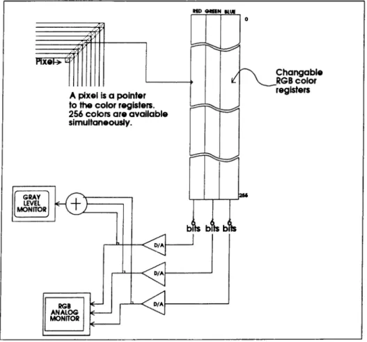
For our specific case, an important system limitation is about the display hardware. The Personal Computer (PC) [4] displays with the regular graphic adapters have a maximum of 1024x760 resolution with the pixel depth of 8 bits. This is a low definition display, and furthermore, the programming language libraries are insufficient even for handling these levels. The Video Graphics

Arrays (VGAs) have a limited number of register bits (specifically 6) assigned for color components. As given on page 7 in [1], there are 64 different choices of levels from the three color components; Red, Green and Blue. This results with obtaining 64x64x64 different colors, however the same card allows the display of at most 256 unique colors of these thousands of colors.

When a monochrome monitor is considered, the situation is even worse. We know (and practically tested) that a monochrome monitor takes the three color components, calculates their exact average and prints that pixel to the screen. In this way, one can easily show that the number of gray tones that can be obtained is 64 + 64 + 64 = 192. Unfortunately none of the standard standard graphic libraries of any programming language and of any compiler producing company supports the utilization of 192 gray tone display on a PC.

№> <MBN HlC

Figure 1.1: Color map installation

The basic problem here is about the standards. The highest resolution the VGA standard supports with 256 colors is only 320x200. Furthermore, 256 colors correspond to 64 tones of gray in the monochrome case. This restriction is because of the small graphic display memory that was available when VGA had became a standard. After the emergence of cheap memory and its applica­ tion to display technology, every company made its own Super Video Graphics

Array (SVGA). Each such SVGA card has a standard part of the VGA and a memory place which can handle higher resolutions. The high memory address is the nonstandard place. A compiler should obviously fail to cope with all the memory addresses that different companies propose. As an example, the SVGA that we use is the one produced by OAK Technologies Inc. For the resolution of 800x600 with 256 colors it has a video frame buffer address starting from AOOO and mode number 54h. We wrote the frame buffer addressing, color map installation and put and get point operations in the low level, i.e. assembly language. In order to obtain the interrupt addresses of 800x600x256 modes corresponding to other SVGA cards, we developed a program depending on the public domain software by Kendall Bennett. That software could figure out the name of the SVGA card installed on the computer, the corresponding interrupt addresses of all present modes and the available memory on the frame buffer. Our program communicates with the modified version of that public domain program and gets the interrupt address of the installed VGA. In this way, we are able to handle the video cards corresponding to most of the known SVGA producers.

Another important limitation directly comes from the operating system of the PC namely “Disk Operating System” (DOS) [7]. Because of the early standardization of DOS, there are very strict memory limitations. It is well known that the main memory area is restricted to 640 K bytes which is normally partitioned to 64 K segments for efficient use of memory. When the program and data size exceeds 64 K, a C user has to change the memory model used in the compiler. Specifically, we used the “large” memory model [8], [9] in the Borland^ C + + compiler. The execution and data access speeds decrease when the memory model increases, but the operating system is still not capable of paging, disk swapping or even extended memory allocation (flat memory). One has to know the exact place of free extended memory in order to use it under DOS. If there are some peripherals using addresses from the extended memory (like the one we have), it is dangerous to make data transfer from extended memory. W ithout knowing the exact allocated memory locations, there is always a possibility of corrupting the functions of peripherals and other extended memory using programs. In terms of conventional memory, the C under DOS has very safe “alloc” and “free” operations [8], [9]. When the memory is not available at the amount of request, the “alloc” function returns an error without causing any more problems. If DOS is used directly without some other environments such as “W INDOW S^^” , it is difficult to be safe under the extended memory. This problem is very disturbing in terms of writing a display software because we cannot read all the large image data as a

2-D array once. This limitation results with the use of disk access all the time during a display operation. For example if the image is scrolled or zoomed, those new parts have to be read from the disk. The use of the display buffer is again not suitable as there are 8 pages of the same memory location on the screen, each of which are 64 K long.

The instruction execution of the PC can also be considered a limitation when compared to mini computers or desktop workstations, however the time required for executing basic instructions like additions, branchings and compar­ isons is not noticeable in the total time required for displaying an image. This shows that instruction speeds of the PC could be ignored in terms of system limitations. The basic speed limit comes from large memory transfers, m ath­ ematical calculations like division or trigonometric operations and operations that require disk access or peripheral device access.

1.2

S y ste m layou t

Hardware:

A brief description of the system is given in the first part of this chapter. Now, the system components will be introduced separately.

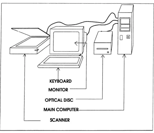
The basic element of the system is the computer, i.e. the PC. The PC that we used has a 80486 microprocessor with a 33MHz clock speed and a total of 4MB ram (1MB conventional 3MB extended) [10]. This 80486 microprocessor has the math co-processor unit in itself, so the multiplications and floating point operations are considerably fast. On the other hand, a PC with a 80386 microprocessor performs as well as the PC that we have because the instruction speed has little effect on the total performance of the system. It is previously explained that the bottlenecks are the memory transfer speed, peripheral access speed, and disk access speed. There is not a noticeable difference between 80386 and 80486 in terms of large memory transfer ( a block of 64KB to some other memory location ) speed. However, because of the better instruction handling, the operations that require loops are faster on a 80486. As a result of this, only the cases for rapid mouse movements and window drawings make the difference between a 80386 and a 80486 in our system.

Beyond the processor, two important units within the computer in terms of speed are the hard disk and the SVGA card. Since disk access is used each

time the image is redrawn on the screen, a fast disk is essential. The speed of the disk is considered in terms of disk access, file position seek and sequen­ tial reading. These operations must all be fast for a good disk performance. Reading 800x600 bytes (480KB) from the file and displaying it on the screen requires about 2.5 seconds with our configuration. The time required for VGA card access and frame buffer allocation on the screen is also included in the given time level.

Figure 1.2: System configuration

The importance of the access speed of the SVGA card emerges immediately when the point put and get operations are considered instead of direct video frame buffer access. Most of the VGA cards have similar operation speeds except for very utilized, special purpose video cards (such as the Targa Board). The one we have is one of those regular SVGAs, so its performance could only be increased by making use of the cache memory. When some amount of the frame memory is assigned to the cache memory, the put point and get point operations become considerably (2 - 2.5 times) faster. The use of cache memory will also be important when peripheral device access speeds are considered. The interface of the optical disk is SCSI and it also makes use of cache buffering if enabled. It is noticeable that application programs like SMARTDRIVE improves the disk access speed performance by the same cache buffering method.

The gray-tone image scanner is connected to the system by a special pur­ pose extension card inserted in the PC. Converse to the cases of image dis­ playing or data-base management softwares, little effort is spent on the image acquisition software. Essentially, the application software that was supplied with the scanner was easy to use and functional. In this program, the image is previewed first, then the appropriate place of the image is marked. After adjusting the resolution of the scan, the user clicks a mouse button to scan the selected part to disk with a chosen file name. An important fact is that, this program supports many image formats including TIFF, so the image formats are compatible between the display and the acquisition software.

Software:

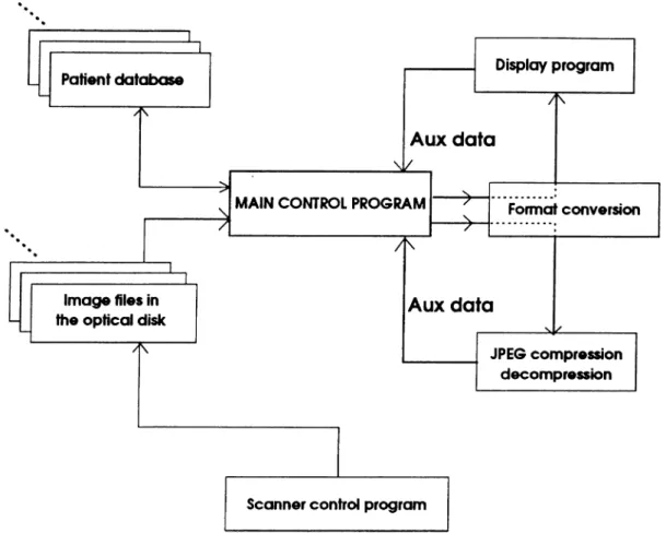
Sharing the same operating environment is a very important issue in terms of user interface. If the user scans the image from a scanner connected to a workstation with the unix operating system and then does the rest of the processing on a PC, the completeness and ease of use of the system would be disturbed. Even on a PC, we have many versions of DOS and other application environments. In order to avoid system mismatches, we specifically converted the environment of all the programs to the MICROSOFT WINDOW S^^. Since the scanner utility program works under WINDOWS, the other programs adopted to it. This environment is suitable in terms of user interface too. The user easily runs the programs, switches from one application to another and exits from the programs by clicking on a mouse button. This is almost ideal for a non-professional computer user such as a radiologist, whom we suppose is the proposed user of our software.

In order to handle the data-base of the radiology images and the owners corresponding to them, a patient record program is developed. Actually, this is the root of the software in terms of hierarchical interface. When the user ex­ ecutes the “Medical Image Workstation” program by pressing a mouse button, he or she first meets a menu asking for an operation on the patient records. These operations are “insertion of a new record”, “seeing the contents of a present record”, “directly going to the image viewing menu”, “changing the record file name”, “creating a record file” , and “exit” respectively. The data­ base program examines a configuration file to learn the name of the record file. This configuration file should be constructed before running. If the “Med­ ical Image Workstation” program (MIW.EXE) cannot find the configuration file, it assumes a default record file name. This record file is made up of 2000 records each of which has six field items, namely, “name” , “age”, “ID number”, “address”, “notes” and “the pointer file for images” . There is no way for the

program to work properly without a record file, so if that file does not exist, the user must create one before doing anything else.

Figure 1.3: Software configuration

When a patient record is written to the file, its place is calculated by a “hash” function applied to the name field. The collision cases are handled in this software and the details will be presented in Chapter 3.

The image viewing and processing part of the software is actually a single program which could be called separately. The integration between the main program and this viewing software is done by executing the viewer from the main program. The data base program has the ability to call the viewer pro­ gram to avoid exiting each time an image viewing is required. It is noticeable that the integration of the two programs is weak. One should ensure that both of the programs together with the compression program are ready at their proper directories before start.

To compress the images, the an implementation of the .Joint Photographic Experts Group (JPEG) standard is executed. This program applies a DCT (discrete cosine transform) based lossy compression on the image. A good feature of this implementation is that the quality - compression ratio trade-off

can be adjusted according to the wills of the user.

The communication between these called programs are done via generating files that are known to all the programs. The necessary data is written in those dummy files. The called program checks those files for information and before termination, it deletes them from the disk. As a result, the user is unaware of these communication files.

Chapter 2

THE IMAGE DISPLAY AND

PROCESSING SOFTWARE

The viewing of the radiological images is one of the two basic elements of this thesis. In the first section of this chapter, the communication between the root “data base” program and the image display program is described shortly. Secondly, we describe the directory management of the display software. Fi­ nally, the displaying functions and supported image operations are described in detail.

2.1

R o o t program - d isp lay p rogram in terface

As mentioned before, the communication between the programs is done by auxiliary files whose names are known to both sides.

One of the record fields is the name of the file which supports the names of the image files corresponding to a patient. This is a text file in which the image file names are written. When the image viewing program “VIEW.EXE” is executed from the root program, it first checks the existence of this “name file” . If this file exists, the program takes the file list from the contents of that file, otherwise it behaves as if it is executed from the prompt and displays a menu which asks the commands to be executed regarding the image files on the disk.

screen. After that, the user travels between those file names either by using the mouse or by using the arrow keys. If the “enter” key or left-mouse-button is pressed on a file name, that file is selected and the program displays the image immediately (if there is no error in the image format). There is a possibility that the selected file is in JPEG compressed form. In this case, the display program generates an auxiliary file indicating the the name of the file to be decompressed and terminates. If the FI key or mid-mouse-button is pressed on a file name and if that file is not a JPEG compressed image, the program generates another auxiliary file to indicate that the file name written is to be compressed, and terminates. Since it is the root program that executes the display program, it goes on running and checks for the image decompression indicator.

If the root program executes the display program after the compression or decompression of an image as indicated above, it generates a different commu­ nication file indicating the name of the compressed / decompressed file. The display program goes to the viewing function in the case of decompression or to the list printing function in the case of compression.

There are two other operations done on the image file list, namely “delete from the list” in the patient image file list mode and “add to the list” which is done when all the directory is searched instead of the patient image file list. However, these operations do not require going back and forth between the two programs. They are done totally in the display program.

2.2

D ir e c to r y m a n a g em en t

The issue of changing directories, listing the image files in a directory and selecting the image files is an almost straight-forward but time consuming and difficult job [4], [7], [10]. It requires system operations which usually causes trouble for the DOS systems. A good directory management might be “a good software engineer’s job”, but we spent little time for smart or understandable programming.

The following is the description of the function “enterJile” called in the display program after checking the auxiliary communication files. Two pa­ rameters come in, namely “image_name” and “flag”, and three go out, namely “xsize”, “ysize” and “header length” . If there is a decompressed image file coming in, then “flag” is set accordingly so that there does not occur any file

start return A ...yes yes — ^ no 1 MENU

quit search change search enter directory

---directory optical disk filename

return

A

Select one

Find the width and length o f the image and obtain the size o f the header in the file

prepare an auxiliary file with the name o f the JPEG file

in it

list printing to the screen, but that decompressed file is selected immediately. In figure 2.1, this situation is indicated by the “single file” branching option. If the flag hcis another value, then it indicates that there is an image file list at the incoming file or there is nothing coming in, so the viewer should display a menu to operate.

The width and height, namely “xsize” and “ysize” are obtained from the headers of the files.

The detailed functional description is not given in the figure because there are lots of situations to handle. The mouse interrupts and return values are obtained from the documentation “GMOUSE.DOC” given with the mouse driver and other low level interrupt codes are found from the appendixes of [8], [9].

Upon the call of “enterJile”, the above function checks the auxiliary infor­ mation and selects an image file as described in the figure 2.1. Briefly, we can define the flow of this function in 5 steps :

1) If no specific list 1.1) Select a directory

1.2) Display the contents of the selected directory 2) Else display the contents of the list

3) Wander around the file names by using the mouse 3) Choose a file from the displayed file names

4) Obtain the header information of the chosen file 5) Return

2.3

C olor m ap in sta lla tio n

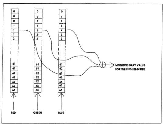
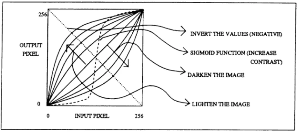
The issue of displaying relatively high number of gray levels with a high hori­ zontal and vertical resolution is perhaps the most important and contributive part of this thesis. In the described method, a total of 192 gray tones can be obtained and this corresponds to 7.3 bits/pel.

There is a need of modification in the color map for displaying the gray scale images on a B/W screen with a SVGA card [1]. The commercially available gray level display programs assign the same value to the color registers to obtain a gray tone [1], [6], but we used the following method for numbering

the color registers

Maximum number of colors = 256 : fixed.

R G B 0 0 0 0 0 1 1 1 1 2 1 1 2 2

In our implementation, we supported a modifiable color map installation in order to be able to make the image brighter, darker, negative, or sharper. During the display mode, the user modifies the color map by pressing “pg-up”, “pg-dn” , “home” , “end” and “insert” keys. Every time these keys are pressed, the following line is executed :

setpalet(setmempalette(map));

with the “map” value determined by the pressed key. The installation of a given color map can also be done in the same way.

The “setmempaletteO” function returns a pointer to the calculated look­ up table which stands for the color map, and the “setpalet()” function installs that table in the video memory by using the DOS interrupt lOh. The necessary register values before the interrupt is defined as follows :

AX=1012h BX=0 CX=256

ES=SEGMENT(table) DX=OFFSET(table)

We assigned six concave up (dark for the normal display) modes indicated by the value of “m ap” from 1 to 6 with 1 having the highest curvature and 6 having an almost linear curve. The concavity is made by taking the powers of the mapping function with values 4, 3, 2.5, 2, 1.7 and 1.3 and normalizing the values for the maximum to be 255. The value 7 is the linear color map curve and it is the default. From 7 to 13, the curve becomes concave down (the image becomes lighter in the normal display) by taking the powers in the opposite way (0.77, 0.6, 0.5, 0.4, 0.33, 0.25). In order to increase contrast, the

map value is assigned to 14. By pressing the “home” key, the value of “map” is reset to the default value, 7.

The negative display is supported independent of the color map adjustment upon pressing the “end” key. Both in the negative and in the normal display mode, the color map is adjustable in the same way.

Figure 2.2: Color map rules

The color map editing is not done manually by changing the curve shape arbitrarily. This would require a separate window to manipulate the color map and since DOS itself is not a multi-window environment, there is not much place to display figures. Furthermore, the restoration of the background after closing a window is not done automatically, so we would either consume a lot of memory to keep the background image or we would redraw the image from the disk. Implementing such a feature would not be worth dealing with these two difficulties. Increasing and decreasing brightness, and increasing the contrast are enough for our viewing purposes.

The function “begingraph()” is called to enter the graphics mode. This function assigns the mode value to the AX register and then calls the interrupt lOh. After that, it installs the color map and assigns a pointer ( “gptO”) to the frame buffer. The desired graphics mode for resolution and pixel depth is determined by the mode number which is an input variable to “begingraph()”. Every SVGA producing company assigns different numbers to different reso­ lution modes. In this program, this function must be called with the specific

Figure 2.3: Changing the color map

variable so that the SVGA enters to 800x600 mode with 256 colors. This re­ quires a memory limit of at least 512K bytes for the display frame. Since this is the beginning of drawing, the function assigns the default color map (7) for color map installation.

To return to text mode, another function “endgraph()” is used. This func­ tion assigns the value “7” to the AX register and calls the DOS interrupt lOh. The value "7" corresponds to the 40x25 text mode with a character cell of 9x16. This is the default monochrome mode at power up.

A normal graphic display does not use our kind of color map installation [1]. The natural way to assign gray tones to 256 colors is to assign equal weighting for all color registers and use the gamma correction. This kind of color map installation results with a total of 64 gray tones and the quantization steps between the gray tones are disturbingly visible for some cases. The following table illustrates the assignments of the color register values with the ordinary method.

Color Register Red Green Blue 0 00 00 00 1 00 00 00 2 00 00 00 3 00 00 00 4 00 00 00 5 01 01 01 6 01 01 01 7 02 02 02 8 03 03 03 9 03 03 03 10 04 04 04 11 05 05 05 58 56 56 56 59 58 58 58 60 59 59 59 61 60 60 60 62 61 61 61 63 63 63 63

Calling the begingraph() function with an appropriate parameter is enough for entering the graphics mode. This parameter determines the resolution and number of colors. W hat is more, it is also possible to change the color map without leaving and re-entering the graphics mode. While the image is being displayed, a function call like “setpalet(setmempalette(7))” results with the loading of the linear color map (the default). In the keystroke control func­ tion, we assigned the pg-up and pg-dn keys for incrementing or decrementing the setmempalette() parameter. In the normal mode, pg-up makes the image brighter and the dark tones are separated better, and pg-dn makes the image darker with the opposite effect. By pressing the “home” key, the default ’7’ parameter is passed and the image becomes normal mapped. To make the image “negative”, “end” key must be pressed and to apply a sigmoid mapping for increasing the contrast, “ins” key must be pressed.

2.4

B a sic p oin t o p era tio n s

Two important functions about a graphics software are the “PutPoint” and “GetPoint” functions [1], [6]. The PutPoint function should put a dot with a given given color to the given screen coordinates. Conversely, the GetPoint function should return the color value of the given coordinates on the screen. The implementation of these functions is considerably simple with the known interrupts. Unfortunately, calling interrupt lOh is not a fast operation, so if one wants to display an image on the screen, he or she should use the frame buffer pointer (gptO) as long as possible. However, during applying some spatial filters, we had to use these functions, so those operations are slow.

For the “PutPoint” function, the the following registers must be set ant the DOS interrupt lOh must be called :

AX = OOFFh & color + OCOOh BX = 0

CX = Xcoordinate DX = Ycoordinate

For the “GetPoint” operation, the following registers are set, AX = OdOOh

CX = Xcoordinate DX = Ycoordinate,

and the DOS interrupt lOh is called. The pixel value is returned in the AX register

Rectangle drawing and mouse cursor drawing are two important utilities that should be considered separately. When the user moves the mouse, the cursor must move on the screen and when a mouse button is pressed, it must behave accordingly. The left button is assigned to put a point, so that when the mouse is moved with keeping that button pressed, one should be able to put a series of points. On the other hand, the mid button is used for drawing a rectangle to indicate the boundaries of operations like filtering, saving etc. In order to draw a rectangle, one must hold the mid button pressed and move the mouse along the diagonal points of this rectangle. Each time the last corner of the rectangle is changed by moving the mouse, the pixels with positions corre­ sponding to the previous rectangle must be reset to their previous values and

a new rectangle must be drawn at the new place. The necessary functions to perform these operations are “getrect()”, “putnewrect()” and “putprevrect()”.

All these functions put and get pixels along the lines corresponding to the borders of the window. The functions obtain the borders from the corners of the rectangle which are passed to the functions as a parameter.

The order of call of these functions is as follows :

putprevrect(oldxl, oldyl, oldx2, oldy2); getrect(newxl,newyl,newx2,newy2); putnewrect(newxl ,newy 1 ,newx2,newy2); oldxl=new xl; oldx2=newx2;

oldyl=new yl; oldy2=newy2;

After that, the new corner coordinates (newx2, newy2) are obtained ac­ cording to the mouse motion.

The motion of the arrow-shaped mouse cursor is handled in a similar man­ ner. When the mouse moves, the old pixel values are restored ( a total of twenty pixels ) and the new arrow is drawn at the new place.

2.5

D ra w in g th e im age

Having defined the frame buffer pointer and the point operations, we can now introduce the image drawing functions. The first of these functions draws the image at its defined size without scaling. If the image size is larger than the screen (800x600), only the fitting part is drawn.

At the beginning of the program, the default setting is such that the up-left corner of the image is at the up-left corner of the screen. When the user presses an arrow key, the image scrolls at the opposite direction at the amount of 40 pixels, but this scrolling is not handled within the drawing functions. When a scroll operation is requested, the main control function simply re-draws the image by passing the horizontal and vertical offsets to the drawing functions as a parameter.

In the first chapter, we had introduced some limitations about the system. Actually, one other limitation is the size of the frame buffer pointer. As a result of being a DOS compatible system, the VGA cards support frame pointers of size 64K bytes. However the size of the screen is obviously more than that, 800 X 600 with one bytes per pixel is 480K bytes. Even if all the screen were available as a single pointer, we would not be able to allocate all of it at once because that would exceed the conventional DOS memory with the program code and other data in the program. Because of these, redisplaying or scrolling the image requires disk accesses every time.

0.0 REGION 1 REGION 2 REGION 3 REGION 4 REGION 5 REGION 6 REGION 7 REGION 8 800,600

Figure 2.4: Screen partitioning

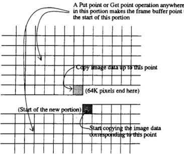
In order to handle the 64K pointers individually, the programmer must be careful about the points where 64K exactly finishes on the screen. At the beginning, the pointer is at the top of the screen starting from the corner position (0,0), and when the pointer index is incremented, it proceeds like (0,1), (0,2), (0,3),... ,etc. Here the convention is (vertical,horizontal). At the 801st index of the pointer, it switches to the position (1,0). In this way, the first 64K finishes at the point (81,735). The frame buffer pointer must switch to the next memory page which corresponds to the place below the first 64K. The switching between the screen portions can be done by a PutPoint or GetPoint operation inside the desired portion. After one of these operations, the pointer starts to point to the first place of the corresponding portion. Actually, the

DOS addresses of all these pages are the same, but the corresponding Put or GetPoint operations cause to change the memory locations inside the VGA card.

Unfortunately most frame pages start from an almost arbitrary points like (81,735), so special care must be taken about the value of the pointer index where it reaches to the end of the buffer.

All of the eight screen portions are handled similarly. The start positions of these portions are as follows :

(0,0), (81,7.35), (163,671), (245,607), (.327,543), (409,479), (492,415), (574,351) There are also some other disturbing points to care about. For example the bottom of every image must be cleared after drawing. This is basically because there could be a scroll up operation, so there could remain some drawn pixels at the bottom.

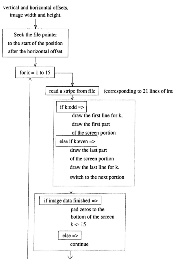
The function described in figure 2.5 draws one pixel per one character in the image file. Although there are 8 portions of 41 lines on the screen, we read half of the data of one portion which corresponds to 21 lines. This is basically because of the memory constraints. If the width of the image is more than 800, we cannot read 41 lines into one array because it exceeds 64K bytes. It is known that the “huge” memory model in the C compilers of the DOS systems support pointers with size larger than 64K bytes, but the memory operations become slow in that case. Because of that, a more practical solution is to stay in a smaller memory model and try to handle pointers with smaller size.

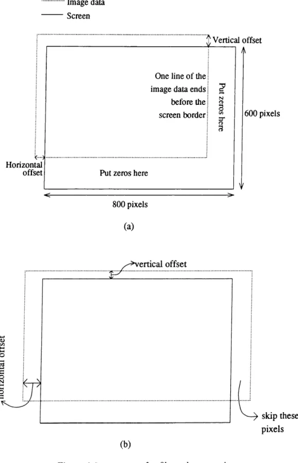
The image borders and the screen borders must be carefully controlled in order to draw the image properly. There are basically two cases to consider for border adjustment (fig. 2.6). In (a), the horizontal data of the image end before the screen border and in (b), there are pixels beyond the screen border. In these situations, the read data must be copied to the frame buffer pointer “gptO” by taking care of the index increments.

Furthermore, we considered the first and last lines of the screen portions individually in order to handle every kind of unexpected situation (fig. 2.7).

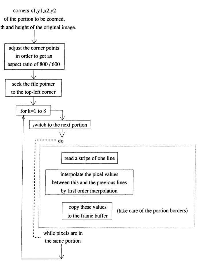
There is also another kind of drawing function which draws the marked region to the screen with magnification. While doing this zoom operation,

vertical and horizontal offsets, im age width and height.

____________

1

Seek the file pointer to the start o f the position after the horizontal offset

fo r k = 1 to 15

'TT

read a stripe from file

ZZ3EZZZZ

(corresponding to 21 lines o f im age)

if k:odd =>

draw the first line for k, draw the first part o f the screen portion else if k:even =>

draw the last part o f the screen portion draw the last line for k. switch to the next portion

if im age data finished => pad zeros to the bottom o f the screen k < - 15

else => continue

\ /

Image data Screen f. Vertical offset <-3t Horizontal offset

One line of the image data ends before the screen border N n> 3 C/3 O 3

Put zeros here

600 pixels 800 pixels

(a)

A Put point or Get point operation anywhere in this portion makes the frame buffer point to the start of this portion

\

'Lc )y 1maj [eU ilal ipl( rOus

(64K pixels end here)

( S t y of the new portion)

Startcof yin

om spo irfii igrti rthis point th ^ image data

Figure 2.7: the end and start points of screen portions

the aspect ratio of the marking rectangle should be considered, so the func­ tion aligns the corner points such that the horizontal size versus vertical size becomes 800 / 600.

A real zooming function should insert necessary amount of zeros between original pixels and then apply a corresponding low pass filter [11], [14]. This is the correct way to do it, but it requires too many computations, so it is extremely slow. In this kind of an application, the user wants to see the result of the operation as soon as possible. Because of this, we preferred to use the simple and fast first-order interpolation. The result is usually satisfactory if one does not apply a zoom with ratio more than three. Figure 2.8 shows the flow diagram of the zoom draw function.

The zoom drawing function is similar to the normal drawing function, but there are more controls. First of all, the corner points of the selected region are modified in order to keep the aspect ratio correct. Other than that, the function reads one line of the image data and makes interpolation calculations on that line and the previous line. The handling of the screen portion switching is done in the same way as in the normal drawing mode, but there are a lot more control statements to consider every kind of situation. The interpolation method is illustrated in figure 2.9. One should note that the fractional pixel positions are rounded to the nearest physical pixel locations and the pixel values are quantized to an integer.

com ers x l,y l,x 2 ,y 2 o f the portion to be zoom ed, width and height o f the original image.

___________ _____________

adjust the com er points in order to get an aspect ratio o f 800 / 600

___________ ____________

seek the file pointer to the top-left com er

A

¿-for k = l to 8

switch to the next portion

do

read a stripe o f one line

interpolate the pixel values between this and the previous lines

by first order interpolation

copy these values to the frame buffer

(take care o f the portion borders)

w hile pixels are in the same portion

_______ \/

linen of the image data a e2= a*yratl + c*yrat2‘ ysize & ePxratl + e2*xratl xsize line-n+1

of the image data

< ... xratl A =pixel value -£3 xrat2 yratl ^|]b*yratl +d*yrat2 ysize

yrat2 = ysize - yratjl

>> II (S o o VO V 800 / (x2 - xl) = xsize

Figure 2.9: first order interpolation >

Because of having long source codes and complex control statements, it is better to give the rough idea of how these functions are implemented instead of explaining the details.

There are actually some graphics routines supported with the compilers, but they are not suitable for our purposes. The best a DOS programmer can do with the standard libraries is the 320x200 mode with 256 colors. If a user is satisfied with this resolution, he or she can draw and manipulate images easily. For example the “Putim age” or “Getimage” functions are ready with most of the compilers.

There are also some specific graphics card producers which distribute a powerful library with the necessary hardware. Usually, these kinds of graphics boards are considerably more expansive than the regular SVGAs. An example for this is the TARGA ^^ board where hundreds of special purpose functions, including displaying, scaling, translation, pixel operations and many more are supported in the distributed software. If this were the case, there would not be a need for developing the preliminary functions for basic operations. Nev­ ertheless, development of these functions is a good exercise about getting into the graphics utilities of computers. The work of this thesis is a chance to see the critical points in low level graphics programming.

2.6

F ilterin g and oth er op eration s

In this section, some basic image processing tools are introduced. These tools include three kinds of low pass filtering, two kinds of high pass filtering, two kinds of median filtering and histogram equalization. All of these filters are applied inside the drawn window and they are 3x3 filters except for histogram equalization. The filter coefficients are calculated according to the rules given in [11] [12] so that the all filters are symmetric and do not cause diffraction-like patterns.

The linear filters essentially apply the following convolution

u(m,n) = ^ ^ a{k,l)y{m — k,n — 1)

{k,l)€W

(2.1)

where y(m,n) and v(m,n) are the input and output images respectively, W is the 3x3 window, and a(k,l) are the filter weights as given in figure 2.10.

All the low pass and high pass filters are done in a single function named “smoothO”. The corner points of the rectangularly marked region and an indicator variable are passed to this function to perform the convolutional filters. The indicator variable can take five different values corresponding to five different filters. These filter coefficients are defined globally as:

/* 3x3 filter coefficients */

float mask[5][3]={ 0.25,0.125,0.0625, /♦ Low pass ♦/ 4.0, -0.5, -0.25, /* High-pass */

0.111111,0.111111,0.111111, /* Averaging */

0.0, 0.2, 0.05, /* Neighbour averaging */

7.0, -1.0, -0.5 }; /* Strong high-pass */

/* . - .

matrix center val__I I I left/right/up/down val___I I matrix corner values__________|

*/

and according to the indicator, the suitable filter is selected. In every row of the two dimensional array “mask[.][.j”, the first value corresponds to the center

of the 3x3 mask, the second value correspond to the neighbors of the center and the last value corresponds to the corners. As a result,

mask[x][0] + 4xmask[x][l] + 4xmask[x][2] = 1

for all filters which is an essential equality for keeping the tone of the image constant.

During applying the 3x3 convolutions, only the necessary amount (3 lines) of the image is taken to the RAM and the operations are performed there. After finishing a line in the selected region, a new line is read from the bottom of the previously read lines. After that the order of the lines are shifted up and the top-most line is thrown away.

3.0623 0.125 3.0623 0.125 3.0623 0.25 0.125 0.125 3.0623 1. Low-pass filter 1 / 9 1 / 9 1 / 9 1 / 9 1 / 9 1 / 9 1 / 9 1 / 9 1 / 9 0.05 0.2 0.05 0.2 0 0.2 0.05 0.2 0.05 3. Neighbour averaging -0.25 -0.5 -0.25 -0.5 4 -0.5 -0.25 -0.5 -0.25 -0.5 -1 -0.5 -1 7 -1 -0.5 -1 -0.5 5. Stronger high pass filter

Figure 2.10: Filter masks

Linear filtering operations are necessary in an imaging program because they are the basic tools for image processing [11], [12], [13], [14]. There are a couple of things to do in order to obtain the coefficients of the low-pass and high-pass filters (page 195 in [11]). The first thing is to determine the specifications. For our purposes, the filter size must be 3x3 and it must be zero phase, so that

= (2.2)

This is equivalent to

for real /i(n i,«2)·

/?,(ni,n2) = A (-n i, -ri2) (2.3)

We used the filter design by windowing method in this work. This method first finds the exact desired impulse response, then multiplies that possibly

infinite impulse response sequence with an appropriate window.

A(ni,n2) = Zld(ni,n2)u;(ni,n2) (2.4)

If h i { n i ,n2) and w{ni^n2) are both symmetric around origin, the resultant

filter will also be symmetric.

The matlab FIR2 command uses the hamming window to calculate the finite impulse response coefficients of the specified filter, and we used that command to obtain the filter coefficients given in the program. Here, the hamming window is give by

w{t) = 0.54 + 0.46cos(7ri/r), if\t\ < T

0, otherwise

(2.5)

for the continuous case. The discrete time case is the time quantized version of this.

Two different kinds of median filtering are implemented in this software [11], [12], [13]. One of them is the regular two dimensional 3x3 median filter­ ing. The other one is applied in a directional manner where the horizontal lines are median filtered in a window of size 3 pixels first, then similar operations are done along the vertical lines in the drawn rectangle window. The regular median filtering causes distortion at the corners of objects in the image, but the directional median conserves those corners. Unfortunately this time the thin lines may possibly vanish. The regular median filter is defined by

u(m, n) = median {y{m — k ,n — /)} , (^·, 1) £ W

(

.

)

We implemented the median selection of the 9 components in the 3x3 case as follows :

- Open an array of size 256 and reset their values to zero - For the pixels in the 3x3 window

- Read the value of a pixel and assign to “a”

- Increment the value of the “a”th indexed element in the array - Get the index of the fifth nonzero element in the array

fifth nonzero index is “1+1” because the summation of the elements up to and including the 1+lst element is five.

0 1 2 3 4 5 6 k-1 k k+1 1-1 1 1+1 252 253 254 255

1 1 1 1 ... 1 2 1 1

Figure 2.11: Finding the median of 9 numbers

On the other hand, the directional median needs only 3 elements, so we obtained the second large value directly by comparing the numbers.

Another process is the histogram equalization [11], [12], [13]. The equal­ ization of the histogram in a marked window is very important especially in radiological images. Usually the dynamic range of the gray tone is poor in these kinds of images, so the digital viewing of them may cause problems. His­ togram equalization is very powerful in this aspect because the details can be separated better if the image tone is almost constant in a region.

In the continuous case, one can exactly make any random variable uniformly distributed over (0,1) as

u = F Ju ) = f pu{u)du

Jo (2.7)

where, Pu(u) is any probability density function. In order to implement this transformation digital images, we calculate the probability of each discrete gray value and call these values Pu{xi) for the gray level xi. If h{xi) is the number of pixels with gray value .r,, then

(2.8)

E.=o*(^.·)

where, L is the number of gray levels. Now we can obtain another set v with the same number of quantization level, L.

S Vu{xi) x,=0

^' = _ 1) + 0.5) _(2.10) 1 ^min

This i>' in general will not be exactly uniform because of being a discrete variable, however its effect on images with poor gray tone range is considerably good in terms of increasing the range of gray tone. Our way of implementing the histogram equalization requires methods similar to the the implementation of the 3x3 median filtering. The past values are first accumulated in an array of 256 and the new values are extracted from that array.

Halftoning may be useful in systems having two level image display monitors [1]. Another place to use halftoning can be two level printing of the images. In the future (when a printer is added to the system), the user might want to print a marked part of the image. In this situation, halftoning (possibly without displaying on the screen) is an essential tool.

The implemented “halftone()” function works in a similar way to the “smoothO” function. We supported two types of halftoning. One applies a comparison with the Bayer Ordered Dither Matrix [1], given as a 2-D array, and the other simply adds a uniform distributed random number to the image pixel values and quantizes to zero or one. Both of the methods are implemented in a single function and the method is choosed by an indicator variable.

The Bayer ordered dither matrix is :

Bayer,,^4 =

15 143 47 175 207 79 239 111 63 191 31 159 254 127 223 95

With this matrix, a constant tone 4x4 region increases its contrast in the following order :

0 0 0 0 1 0 0 0 1 0 0 0 1 0 1 0 0 0 0 0 0 0 0 0 0 0 0 0 0 0 0 0 0 0 0 0 0 0 0 0 0 0 1 0 0 0 1 0 0 0 0 0 0 0 0 0 0 0 0 0 0 0 0 0

1 0 1 0 0 0 0 0 1 0 1 0 0 0 0 0 1 0 1 0 0 1 0 0 1 0 1 0 0 0 0 0 1 0 1 0 0 1 0 0 1 0 1 0 0 0 0 1 1 0 1 0 0 1 0 1 1 0 1 0 0 0 0 1 1 0 1 0 0 1 0 1 1 0 1 0 0 1 0 1 1 1 1 0 0 1 0 1 1 0 1 0 0 1 0 1 1 1 1 0 0 1 0 1 1 0 1 1 0 1 0 1 1 1 1 1 0 1 0 1 1 0 1 1 0 1 0 1 1 1 1 1 0 1 0 1 1 1 1 1 0 1 0 1 1 1 1 1 1 1 0 1 1 1 1 1 0 1 0 1 1 1 1 1 1 1 0 1 1 1 1 1 0 1 1 1 1 1 1 1 1 1 1 1 1 1 1 1 0 1 1 1 1 1 1 1 1 1 1 1 1 1 1 1 1 1 1 1

According to the application, the Bayer matrix or random noise addition can be used.

2.7

D ifferent screen u tilitie s

There are a few screen utilities which are essential for a viewing program. The first one is the utility to save an indicated portion of a possibly modified image from the screen to the disk.

The save operation is done by writing the pixel values to the disk with the “putc(value,outfile)” command of the C compiler in the PPM format. The selected region is first saved to an auxiliary file. The name of the file to save as is asked to the user and then that file is renamed to have the indicated name.

The next utility is the calculation of the area inside a closed contour de­ fined by putting points with the mouse ( figure 2.12 shows how this is done graphically) [15]. This is possibly a useful utility for the radiological users. The application may arise when the same tissue of the same person can be examined at different times. The doctor may want to see if there is a change in the size of a region. After marking the surroundings of a specified part, the following function calculates the inner area by approximating the green’s

integral for the discrete case. In between the sequential points, we assume a line connecting them, and the last point is assumed to be connected to the first point in the index with a line. The unit of area is the number of pixels in the original scale. If the Image is magnified, the function that calls the find_area routine takes care of the scaling, so there is no confusion in terms of the area. Unfortunately, the user must consider the scaling during the scanning opera­ tion. If the two images are scanned in two different scales, there is no reason to compare the two areas in those images.

have this link. S ii^ ra o / this length w hile go in g n gh t

Add this length w hile goin g left

Figure 2.12: Finding the area

Another utility about the user interface point of view is being able to write text on the graphics screen. If the user wants to put some labels on some places, he or she can press the “T” key at any mouse position and write anything by using the keyboard. When an “enter” is pressed, the text mode finishes and any pressed key becomes the operation, like “Z = zoom”, “S = L.P.F.” in the normal mode. After drawing an arc shaped arrow by putting points, the label can be typed to indicate the contents of the place the arrow is positioning. After that, these changes can be saved by using the “save_screen()” function which is called after drawing a rectangle to indicate the borders and pressing “D”. This enables us to store the modified images. These modifications include any kind of filtering, histogram equalization, halftoning, point drawing and text inserting. Color map modification is not a direct modification on the image data, so that information cannot be saved.

Now we will briefly describe the WriteText() function which outputs a text on the graphics display. It uses the ROM BIOS data to find out the shapes of the ASCII characters and then puts points on the filled positions for each