High Tc superconductivity

A T H E S I S S U B M I T T E D T O T H E D E P A R T M E N T O F P H Y S I C S A N D T H E I N S T I T U T E O F E N G I N E E R I N G A N D S C I E N C E O F B I L K E N T U N I V E R S I T Y I N P A R T I A L F U L F I L L M E N T O F T H E R E Q U I R E M E N T S F O R T H E D E G R E E O F M A S T E R O F S C I E N C E

By

taraflıdan ba^ışiannuştır.

¿ X м г . s ?

н п / с . <

I certify that I have read this thesis and that in my opinion it is fully adequate, in scope and in quality, as a thesis for the degree of Master of Science.

Prof. Dr. Salim Çıracı(Principal Advisor)

I certify that I have read this thesis and that in my opinion it is fully adequate, in scope and in quality, as a thesis for the degree of Master of Science.

Prof. Dr. Cemal Yalabık

I certify that I have read this thesis and that in my opinion it is fully adequate, in scope and in quality, as a thesis for the degree o f Master of Science.

Prof. Dr. Şinasi Ellialtioglu

Approved for the Institute of Engineering and Science:

Prof. Dr. Mehmet JBeray,

ABSTRACT

H IG H

T c

M . Zafer Gedik M . S. in Physics

Supervisor: Prof. Dr. Salim Çıracı December, 1989

A critical summary of the recent developments in high temperature super­ conductivity is given. Physical properties of the new materials are summarized.

The new theories proposed to explain high Tc are reviewed. In the case of a

special type anisotropic gap, the currents and conductivity for single particle

tunneling in high Tc superconductor junctions are calculated. Tunneling is as­

sumed to be specular. The position of the peak in the conductivity curve, is found to be determined by the shape of the Fermi surface. Two geometries

are considered: tunneling paxallel and perpendicular to CuO^ planes. The

order of the peaks for these two configurations turns out to be opposite to experimental results. It is concluded that, conventional one band theory of superconductivity is not enough to explain observed tunneling spectra of high

Tc superconductors.

Keywords: Superconductivity, anisotropic gap, high temperature supercon­ ductivity, tunneling.

Y Ü K S E K

T c

M . Zafer Gedik Fizik Yüksek Lisans

Tez Yöneticisi: Prof. Dr. Salim Çıracı Aralık, 1989

Yüksek sıcaklık üstüniletkenliğindeki son gelişmelerin bir tekrarı yapıldı. Yeni malzemelerin fiziksel özellikleri özetlendi. Yüksek Tc’yi açıklamak amacıyla ileri sürülen yeni teoriler anlatıldı. Özel bir yönser axalık durumunda, yüksek

Tc üstüniletkenlerinden yapılan eklemlerde, tek parçacık tünellemesi için akım

ve iletkenlik hesaplandı. Tünellemenin düzgün olduğu varsayıldı. İletkenlik eğrisindeki tepenin konumunun, Fermi yüzeyinin şekliyle belirlendiği bulundu.

İki geometri göz önüne alındı; CuÖ2 düzlemlerine koşut ve dik tünelleme.

Bu iki konum için bulunan tepe konumlarının sırasının, deneysel sonuçlara ters düştüğü görüldü. Tek kuşak üstüniletkenlik teorisinin, gözlenen tünelleme izgelerini açıklamaya yeterli olmadığı sonucuna varıldı.

Anahtar kelimeler : Üstüniletkenlik, yönser aralık, yüksek sıcaklık üstüni­ letkenlik, tünelleme.

ACKNOWLEDGEMENT

It is my pleasure to express deep gratitude to my supervisor, Prof. Salim Çıracı, for his guidance and suggestions throughout the development of this study. I would like to thank to Prof. Toni Schneider and Martin Frick for stimulating discussions. I greatly appreciate Oğuz Gülseren for his valuble comments and helps in typing this thesis. Lastly, I would like to thank to Erkan Tekman for his remarks and moral support.

A b s t r a c t ... iii

Ö zetçe I V A c k n o w le d g e m e n t ... v

C o n t e n t s ... vi

List o f Figures ...viii

List o f Tables Xll

1 INTRODUCTION

2 CONVENTIONAL SUPERCONDUCTIVITY

2.3.2 Strong Coupling Theory 30

3 HIGH TEMPERATURE SUPERCONDUCTORS

32

CONTENTS 3.3 Y / B a / C u / 0 ... 47 3.4 B i/S r/C a /C u /0 and T l / B a / C a / C u / 0 ... 58 3.5 K / B a / B i / 0 ... 65 3.6 N d / C e / C u / 0 ... 66 3.7 P b / S r / Y / C u / 0 ... 67

4 THEORIES

70

4.1.1 Phonons, B ip ola ron s... 71

4.1.2 Plasmons, Excitons, Polarization Waves . 76 4.1.3 Magnons and Spin Waves ... 85

4.2 t-J M o d e l ... 89

5 SINGLE PARTICLE TUNNELING

5.2 Uniaxial Anisotropy 106

5.3 E x p erim en t...I l l

6 Conclusions

115

1.1 Highest Tc versus time

2.1 Resistivity versus temperature for mercury

2.2 Thermal conductivity versus temperature for two cases 2.3 Critical field versus temperature

2.4 Type I (A) and type II (B,C,D) superconductors 2.5 Temperature dependence of energy gap A

2.6 Tunneling current from a normal metal into a superconductor 10

2.7 Two possible paths to calculate the wave function ... 11

2.8 Surface resistance of a su p ercon d u ctor... 12

2.9 Electronic specific heat versus te m p e ra tu re ... 12

2.10 Isotope e f f e c t ... 13

2.11 A two dimensional picture o f k-space... 17

2.12 Coupling of electrons via phonon exchange... 18

2.13 Excitation spectrum for BCS ground s ta te ... 25

2.14 Density of states in the superconducting phase 30 3.1 Perovskite s tr u c t u r e ... 34

LIST OF FIGURES IX

3.2 Phase diagram of B a P b i-xB ixO z... 34

3.3 Band structure of BaPby-xBixOz 36

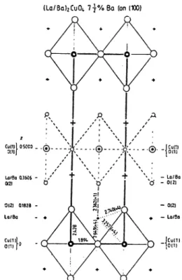
3.4 Crystal structure of Lai.zbBao,izCuOA... 37

3.5 Interatomic distances of 2 -1 -4 38

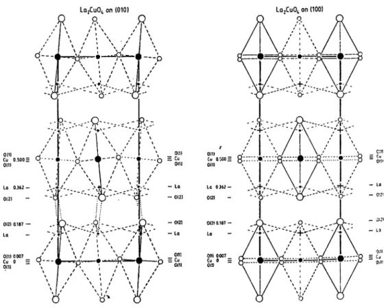
3.6 Orthorhombic distortion 39

3.7 Phase diagram for Laz-xSrxCuO^-y 40

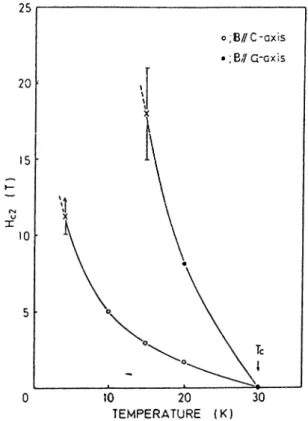
3.8 Neutron scattering results for 2 - 1 - 4 ... 41 3.9 The magnetic structure of 2 - 1 - 4 ... 41 3.10 Upper critical fields of 2 -1 -4 ... 42

3.11 Band structure of 2-1 -4 43

3.12 Schematic picture of formation of C u -0 b a n d s ... 44

3.13 Calculated density of states for 2 -1-4 ... 44

3.14 Valence band photoemission spectra for 2 - 1 - 4 ... 45

3.15 Resonant photoemission spectra for 2 -1 -4 46

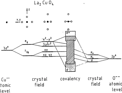
3.16 Schematic energy level d ia g ra m ... 46

3.17 Crystal structure of 1-2-3 compound 48

3.18 Phase diagram of 1-2-3 compound 49

3.19 Magnetic structure for 1 - 2 - 3 ... 51 3.20 Resistivity o f 1-2-3 versus te m p e ra tu re ... 52

3.21 Calculated LDA bands for Y B a ^ C u z O j...- 52

3.22 Total and partial density of states of 1-2-3 54

3.24 X -ray absorption near edge structure of 1-2-3 55

3.25 Flux quantization for 1-2-3 56

3.26 Upper critical field of 1 - 2 - 3 ... 57

3.27 Specific heat of YBa-iCuzOr versus temperature 58

3.28 Crystal structures of Tl compounds 60

3.29 Crystal structure of ^ ¿ 2 2 1 2 ... 61

3.30 Transition temperature versus filling f a c t o r ... 62

3.31 LAPW energy bands for Bi 2212 63

3.32 Band structure of T/2201 ... 64

3.33 Total and projected density of states for Bα/71íΓ/Bг‘/ 0 . . . . 65

3.34 Crystal structures of electron superconductors 66

3.35 O — Is absorption edge o f Nd2~xCexCu0 4... 67

3.36 Crystal structure of _Ph2Sr2MCuzOs 68

3.37 Energy bands for Pb2Sr2YCus08 69

4.1 Calculated values of u and Tg o f La2-xMxCu0 4 ... 72

4.2 Formation of the bipolaxon from small p ola ron s... 74

4.3 Energy dispersion relation for bipolaxons... 76

4.4 Pairing of electrons via excitons in a dielectric medium . . . . 82

4.5 Energy level diagram for Cu d and O p states 83

4.6 Interaction potential for the Harrison model

86

4.7 Electron-magnon coupling d ia g ra m s ... 87

LIST OF FIGURES XI

4.9 Hole p rop a g a tion ... 91

4.10 Aharony m o d e l ... 92

4.11 Phase diagram for t-J model 95 4.12 Short range RVB con figu ra tion ... 97

4.13 Phase diagram for fermionic representation 99 4.14 Tunneling conductance 100 4.15 Holon p a ir in g ... 101

5.1 Fermi s u r fa c e ... 107

5.2 Calculated NISPAR con d u ctiv ity ... 108

5.3 Density of states for an anisotropic superconductor... 110

5.4 Calculated SIS current versus voltage... 110

5.5 Tunneling spectroscopy for 1 - 2 - 3 ... 112

3.1 Oxide superconductors 33 3.2 Tl/Ba/Cu/0 co m p o u n d s... 59

4.1 Paxameters of the Emery Hamiltonian 89

5.1 NISPAR and NISPER peaks ... 114

Chapter 1

IN T R O D U C T IO N

A breakthrough in the field of superconductivity has taken place in the past three years. The critical temperature below which the material becomes

superconductor has risen from 23 K to 125 K. It had been already known

that many metals, alloys and some semiconductors when cooled to extremely

low temperatures as low as 20 K transport electrical current with virtually

no loss, but only in 1987 it became possible to obtain superconductivity with the use o f inexpensive and easily available nitrogen rather than expensive and complex helium cooling systems. Interestingly, the materials causing this excitement were not metals but some oxides.

The liquefaction o f helium by Heike Kamerlingh Onnes was the first step towards superconductivity. Upon cooling the resistance of a normal metal falls rather rapidly first and then levels off to a constant residual value which depends on the amount of the impurity present. In a series of experiments on electrical resistivity Onnes[l] observed that mercury deviates from this behavior and its resistance abruptly vanishes within a fraction of a degree

change o f temperature at 4.15 K . In 1913, Onnes received Nobel Prize in

Physics for his investigations of the properties of matter at low tempera­ tures. Since the discovery of this phenomenon in 1911, there has been great efforts both in the discovery of new superconductors and in the explana,tion of superconductivity.

A satisfactory microscopic theory of superconductivity was put forward in 1957, 46 years after the discovery o f superconductors, by John Bardeen, Leon

Cooper and Robert Schrieifer[2] and they received the Nobel Prize in Physics in 1972. This theory was a result of a lot of work and effort preceding it. Gorter and Casimir[3] developed the thermodynamics of the superconduct­ ing state. London brothers[4] and Pippard[5] studied the electromagnetic properties. Ginzburg and Landau[6] put forward a phenomenological the­ ory which can be derived from the microscopic theory of Bardeen, Cooper and Schrieffer as shown by Gor’kov[7]. An important step was the discov­ ery of superfluidity of helium, its frictionless flow through narrow slits and

capillaries, in 1938. Physical properties of liquid phases of He^ and

were completely different. Then the relation between Bose-Einstein conden­ sation and superfluidity became clear. Electrons in a metal could produce a Bose system, for example by binding in pairs with zero spin. Implications of this idea had been studied by many researchers earlier, but a complete theory with an explanation of the pairing mechanism had not been found until 1957. Results of the Bardeen-Cooper-Schrieffer theory have been red­ erived by Bogoliubov[8] using a different method. Eliashberg[9] extended this theory based on the phonon pairing mechanism which was applicable to weak coupling superconductors in its original form , to strong coupling superconductivity by introducing retardation effects. With the discovery of high temperature superconductors initiated by Johannes Georg Bednorz and Karl Alex Miiller[10] a new field was opened in superconductivity. Apart from their technological importance, high temperature superconductors have raised some questions on the validity of the classical theories. Main reason

for these suspicions was simply the fact that Tc was too high. Bednorz and

Miiller shared 1987 Nobel Prize in Physics while thousands of physicists were studying in their laboratories to And new materials possibly with even higher critical temperatures and almost the same number of theoreticians were spec­ ulating on the mechanism of superconductivity observed in these materials.

High Tc materials justified the fact once more that: superconductivity is still

one o f the outstanding puzzles of physics.

Absence of resistance to flow of electricity is the most important property of superconductors for practical purposes. However there axe three main obstacles: smallness o f the critical temperature and the critical current, and destruction o f superconductivity under a strong magnetic fleld. The rise

of the highest critical temperature Tc in years is presented in the following

CHAPTER 1. INTRODUCTION 130 120 110 100 00 80 g 70 60 50 . 40 30 20 10 0 , n « 1-3 A = Bl orTI M = Sr or Ba O YBa^Cu^Oy • (La,Sr)2Cu04 NbQGe Nb3$n o NbN qO O · Ba(Pb,BI)03 Pb Nbo r? '' <5rTin · Bronx·· Ohq SrTIÜ3.jf ' J____flU . 1910 1930 1950 1970 1900

Figure 1.1: Highest Tc versus time

Materials having greater than 77.4 K can be cooled with nitrogen[ll].

Oxide superconductors have been known since 1964. After the pioneering

discovery of (L a,B a)2Cu04 with Tc=Z5 K by Bednorz and Muller the first

nitrogen superconductor Y B a2Cu3 0 j was found in 1987(12]. The importance

of the discovery of yHaaCusOr is that it becomes superconducting above the

boiling point o f the nitrogen, T=77.4 K , under the normal pressure, and that

is why we called it nitrogen superconductor.

In small scale applications of superconductors, tunneling is a very im­ portant phenomenon. This technique was pioneered by Giaver[13j. Subse­ quently, a very interesting manifestation of quantum mechanics was predicted by Josephson[14] for two superconductors which axe separated by a thin oxide layer. In 1973, Ivax Giaver and Brian D. Josephson received the Nobel Prize in Physics.

medical magnetic resonance imaging (MRI), high energy physics, high field magnets for scientific applications and magnetic separation. Although the first superconductive MRI was constructed in 1980, it has already become the dominant market for superconductors. The strong magnetic fields needed in accelerators or in nuclear magnetic resonance (NMR) experiments are created by superconducting coils. Nowadays, it is possible to separate minerals by magnetic field gradients for purification purposes.

There are also yet uncommercialized applications of superconducting mag­ nets: fusion by magnetic confinement, motors and generators, energy stor­ age systems, levitated trains-MAGLEV, magnetohydrodynamics, magnetic launchers, magnetic refrigeration, crystal growth and ships moving with the force between a magnet and electric current passing through the sea wa­ ter. Superconducting transmission lines have the ability to carry significantly more current without power loss due to the resistance. Superconductors can also be used in construction of smaller and faster computers. Superconduct­ ing Quantum Interference Device (SQUID) is the most sensitive detector of electromagnetic signals known. An antenna made of high temperature superconductor can be as small as 5% of the size required for conventional antenna. Superconducting optical switches have been produced. Radio waves with wavelength of the order of millimeter have been detected by Josephson

junctions made oiY B aC uO thin films. It is expected to double the available

frequency range for communications. Probably a number of other application areas that we have not mention here will appear in the future.

This thesis is a brief review o f the current status of superconductivity along with an application of conventional tunneling theory to high temper­ ature superconductors. The second chapter contains the fundamental prop­ erties o f conventional superconductors and theories proposed to explain su­ perconductivity. We review the high temperature superconductors with their common properties in the third chapter. The proposed mechanisms for high

Tc are reviewed in the fourth chapter. In the fifth chapter we calculate the

tunneling conductivities for a model of new materials. Finally in the sixth chapter we present our conclusions.

Chapter 2

C O N V E N T IO N A L

S U P E R C O N D U C T IV IT Y

2.1

Experimental Observations

Superconductors, as their name implies, conduct DC currents without

any dissipation below a certain temperature Tc (Fig. 2.1). Resistive effects

reappear in the microwave region. At T = 0 JiT no absorption is observed until

the critical frequency Wc, where fiojc = 3.5fcTc. This frequency corresponds to

wavelengths of the order of 1 mm. Te is generally of the order of a few degree

K , but it can be as large as 20 to 30 K . It should be noted that due the

thermal fluctuations resistance may not be zero though it is extremely small

below To, and there may also be a superconducting phase above the critical

temperature. These fluctuations are reflected also in magnetic properties. On the other hand superconductors are not perfect thermal conductors.

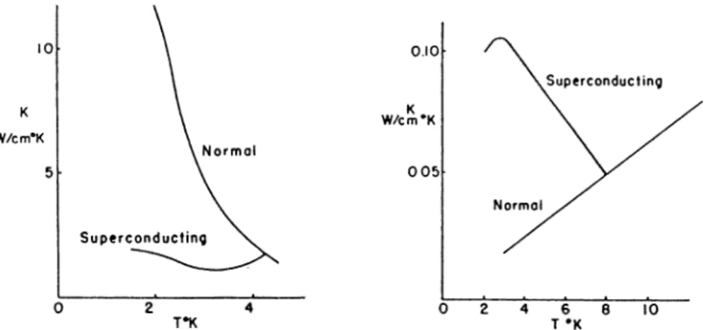
Thermal conductivity in the superconducting S phase may be even smaller

than that in the normal N phase as shown in Fig. 2.2.

Another very important characteristics is perfect diamagnetism which is responsible for the fact that magnetic fields cannot penetrate into supercon­ ducting material up to a temperature dependent characteristic distance A, the so called penetration depth. This is of the order of hundreds of angstroms. Repulsion of magnetic flux is known as Meissner effect. Using microwave

r 0 h ---•n't : j 1 r---' i.· \ r ___ )J. ____\'Tc

Figure 2.1: Resistivity versus temperature for mercury

This figure is taken from the original work of Onnes[l].

Figure 2.2: Thermal conductivity versus temperature for two cases

(a) Mercury[15] (b)Lead-10% bismuth alloy[16]

techniques, changes in A = A(T) can be measured accurately. It is difficult to devise a method which can determine the absolute value of A(T) precisely. In experiment one usually fits A(T) to a reference value which is obtained from theory. It is also possible to use superconducting quantum interference devices (SQUID’s) to measure penetration depth with a precision equal to

CHAPTER 2. CONVENTIONAL SUPERCONDUCTIVITY

that of microwave techniques.

If the magnetic field is very strong superconductivity may be destroyed

(Fig. 2.3). As a result of this there is a critical current Jc for every material

which creates the critical field He. Critical current is of the order of 10® to

10® kfem^ at 0 K .

Figure 2.3: Critical field versus temperature

Ho, the value at which the curves intersect the perpendicular axis, changes from 10

to 10®(j. The region in which the material is superconductor lies below the curve[17].

According to their behavior in a magnetic field one distinguishes two types of superconductors: Type I and Type II. The previous graph showing the temperature dependence of the critical magnetic field is characteristic of a type I superconductor. For the so called type II superconductors there are two critical values for magnetic field. Between these two, magnetic flux can partially penetrate through the substance (Fig. 2.4). This state contains both superconducting and normal regions, vortices, and the sample is said to be in the mixed state or the vortex state. Since there are circulating currents around these normal regions and the direction of circulation is the same for all, two vortices repel each other. Below the so called lower critical

field Hci, whose typical value is 500 G, the flux is excluded completely. If

the applied field is increased from Hd, the number of vórtices increases and

therefore they start to interact with each other. It turns out that lowest energy configuration for these vortices is a two dimensional triangular lattice.

is destroyed. Upper critical field is generally a large value (~ at 0

K ) and that is why type II superconductors have wide areas of application.

There is also another, critical field called Hcs- When the field exceeds _Hc2 bulk

superconductivity disappears but if the field is parallel to the surface of the material there is still a superconducting layer on the surface. This behavior

continues up to Hcs- All critical fields decrease from their maximum value

at 0 K to zero H at Tc. In measurements, materials are of the shape of long

cylinders and the magnetic field is parallel to the axis of the cylinder.

600 400 200 «

/

Applied magnetic field Ba in gauss

2800 3200 36001

Figure 2.4: Type I (A) and type II (B,C,D) superconductors

Below the critical field (the lower critical field for type II) the magnetization is equal in magnitude to the applied field but it is in the opposite direction therefore

the net field inside the superconductor is zero (After Livingston) [17].

Almost all superconductors have an energy gap Eg = 2A which is to be

overcome to destroy the superconducting (S) phzise. Eg is normally in the

range of But some materials which contain magnetic impurities

show superconductivity without an energy gap. When the concentration of magnetic impurities is increased the gap value is decreased till zero. This is the criticed impurity concentration after which superconductivity is not observed. Temperature dependence of energy gap is shown in Fig. 2.5. Below

Tc we need a nonzero energy to destroy the superconducting state. As the

temperature is increased from zero the superconducting gap decreases and finally vanishes at the critical temperature.

Existence of an energy gap in the excitation spectrum o f a superconduc­ tor was first proposed by Bardeen, Cooper and Schrieffer in their theory.

CHAPTER 2. CONVENTIONAL SUPERCONDUCTIVITY

Figure 2.5: Temperature dependence of energy gap A

Weak coupling supercondcutors follow almost the same temperature dependence predicted by BCS theory (After Townsend and Sutton)[17].

Later this speculation was verified experimentally. A direct way of measur­ ing the energy gap is electron tunneling method. In tunneling experiment not only the width of the gap, but also density of states in the superconducting phase can be measured. Consider a metal-insulator-metal junction. When the both metals are normal, the junction exhibits an ohmic behavior at low temperatures[18,19]. If one of the metals becomes superconductor, current- voltage characteristic changes (Fig. 2.6)[13]. In a superconductor, electrons axe paired, therefore, charge of the current carriers is 2e rather than e. Since there is a gap at the Fermi level in the superconducting phase, at absolute zero, i.e., in the absence of normal electrons, no current can flow through the

junction unless the applied potential V exceeds Vc = Eg/2e = A /e .

When both metals are superconducting we obtain a Josephson junction which not only shows fascinating results of quantum mechanics but also has wide range of applications. Superconductors therefore axe very interesting because the quantum mechanical effects axe observed at macroscopic scale. Flux quantization is one of these phenomena. Inside a superconductor the

Figure 2.6: Tunneling current from a normal metal into a superconductor

With increasing temperature the curve approaches to normal state current-voltage relation, i.e., Ohm’s law[20].

magnetic field is zero, therefore, the vector potential is of the form A = V / where / is a well- behaved arbitrary scalar field. By a gauge invariance argu­ ment, namely by assuming that physically observable quantity, the absolute square of the wave function is independent of the choice of / , it is easy to

show that the wave function is of the form

(

)

where

f ( r , t ) = I df^’ A{f^,t) (2)

Assume that we want to find the wave function inside a superconductor by

a knowledge of its value at the origin. X f )

We can calculate the value of ^ at r using either path! or path2)\l^\i we

require that the electron wave function is single valued then g-S^(/l+/2) = 1 =: e2irm

or

/ i + /2 = jd f * · A(r, t)

(3)

CHAPTER 2. CONVENTIONAL SUPERCONDUCTIVITY 11

Figure 2.7: Two possible paths to calculate the wave function

The value of the wave function at f can be calculated if its value at fo is known. However different paths will give different values[21].

=

X

Here S is any surface bounded by pat hi and path2 . Thus flux is quan­

tized. In fact this expectation has been verified by experiment with a slight modification, e is replaced with 2e. In other words current carriers are not electrons but electron pairs. As we may guess flux passing through the nor­ mal regions o f type II superconductors in the mixed state is also quantized. This explains why the number of vortices increases with the increasing mag­ netic field. Because there is only one flux quantum in the normeil core of each vortex.

Since there is a gap in the electronic density of states, photons of energy less than the gap energy are not observed. For such photons the resistivity o f the superconductor vanishes at absolute zero. At high frequencies resis­ tivity approaches that of a normal metal because high energy photons cau^e

transitions from S to N state (Fig. 2.8).

Since two different phases can be associated with the normal and super­ conducting state, there occurs a second order phase transition. This can be

Figure 2.8: Surface resistance of a superconductor

This graph shows the difference of normal and superconductor surface resistances versus frequency of far infrared photons. There is a threshold at the gap edge

(After Richards and Tinkham)[17].

seen from the variation o f the electronic specific heat Ces with respect to the

temperature (Fig. 2.9). Ce«, specific heat due to electrons in the supercon­ ducting state, changes exponentially at low temperatures. Flatness of the curve as temperature goes to zero is a result of energy gap.

c,,.lyTr.

T i r

Figure 2.9: Electronic specific heat versus temperature

At the critical temperature Tc a discontinuity is observed. 7 is the constant in the

normal specific heat relation Cen = 7i ’[22].

The most important experimental clue for the role of phonons in super­ conductivity is the isotope effect. It is observed that critical temperature

CHAPTER 2. CONVENTIONAL SUPERCONDUCTIVITY 13

varies with isotopic mass as

M°‘Tc = constant

(

)

This becomes clear in Fig. 2.10 which presents log-log plot of transition temperature versus average meiss number for separated isotopes of mercury.

Critical temperature of mercury is inversely proportional to square root of the mass of the isotope[23].

Mechanical properties of material also change when it becomes supercon­ ductor, but these changes axe very small in comparison to drastic changes in the electrical and thermal properties. Under pressure criticad temperature increases.

2.2

Ginzburg—Landau Theory

Basic electrodynamic properties of superconductors were well explained by F. London and H. London[4] starting with two basic equations. In the London theory, the density o f superconducting electrons is assumed to be constant throughout the space and the basic equations are local, namely that they relate the electric and magnetic fields at a point to the value of current density at the same point. In 1953 Pippard[5] introduced the concept of coherence length while proposing a nonlocal generalization of the London theory. Pippard’s electrodynamics current density at a particular point is

given in terms of an integral of the vector potential. The main contribution to this integral comes from those points whose distances to this particular

point are less than the coherence length In fact ^ is a measure of the

dimension of electron pair or the so called Cooper pair.

Ginzburg-Landau theory[6] is a generalization of the London theory to inhomogeneous situations. It is very difficult to handle spatially varying problems by microscopic theory which will be described in the next sec­ tion. Ginzburg-Landau theory was given limited attention until 1959 when Gor’kov[7] showed that it was derivable from the microscopic theory as a special case. Initially it was applicable to problems near the transition tem­ perature under the low magnetic fields, but later it has been extended to arbitrary temperatures and high fields. Ginzburg-Landau theory has also been improved to handle time-dependent phenomena.

Let the density of superconducting electrons at a point f be given by

where the order parameter is properly normalized. Near the

critical temperature is expected to be small, therefore, we can expand

the free energy density Fs in the S state as

Fs{<e,T) = Fk + + i;8 (r)| i| ‘

(

₇

)

Minimizing Fs with respect to ji'P we obtain the equilibrium order parameter

to be

l* .P =

ßiT)·

(

)

Free energy difference between normal phase N and superconducting phase

S should be equal to the energy of the magnetic field

„ 1 a(T) HHT)

(9)

(

)

depth is inversely proportional to the density of S electrons, oc ^ then

A^(0) _ |^e(T)p _ g ( r )

A2(T) |i-E(0)|2 ß{T)

Therefore, by solving a{T) and ß{T) in terms of experimentally measurable

quantities one obtains

H^{T) X^T) 4ir A2(0) H^(T) X\T) 47t A4(0) c,(T) = ß(T) = (11) (12)

CHAPTER 2. CONVENTIONAL SUPERCONDUCTIVITY 15

When i'(f3 is not uniform we add a gauge invariant term to the free energy. Thus

= i^5 + - - A W (13)

where A is the external vector potential, e* is the charge of the particles

forming the S phase. Minimizing the free energy with respect to i'* and A

with appropriate boundary conditions we obtain four equations forming the basis of the Ginzburg-Landau theory

2m ^ c ^ 0Φ* = 0 2 7 fie * h ...^ - τΛτ * \ 47re*^, _ r* „ i t -(Φ*νΦ - ΦνΦ*) + — 3 ~|Φ| A = ^ A me mc^ V ’ A = 0 n - ( - i n V--- Α)Φ = 0 c (14) (15) (16) (17)

In this equation n is the unit vector normal to boundary separating S and

N pheises. Defining the following parameters

2e*2 «2 = -Λο — ____772\4 me* 4πβ*Φ? (18) (19)

we see that there are three quantities k, A, Ho to be determined. However,

since we know that e* = 2e, only two of them are independent.

2.3

Microscopic Theory

Although superconductivity was discovered in 1911, a successful theory has been proposed 46 year later by J.Bardeen, L.N.Cooper and J.R.Schrieffer[2]. Until that time many phenomenological theories some of which we mentioned above had been proposed[24]. Theory of Bardeen, Cooper and Schrieffer is very successful in describing physical properties o f weak superconductors in which strength o f the electron-phonon interaction is small. For example, one can very well explain the superconductivity of aluminum within this formal­ ism. In 1960 Eliashberg[9] improved this theory by extending to cover strong

electron-phonon coupling (as in the case of Pb) and to handle retardation

2.3.1

Weak Coupling Theory

The basic hypothesis of Bardeen-Cooper-Schrieffer (BCS) theory is that

in the superconducting state electrons occupying k and —k states are paired

through lattice vibrations and when an electron is scattered from k to k',

its partner —k is simultaneously scattered to —P. Therefore, either both k

and —k are occupied or they axe simultaneously empty. This is the second

important property of the superconducting state in addition to the presence of an attractive interaction between the electrons. In a normal metal scattering of different electrons via phonons, impurities, etc., are independent of each other and that is why there is a finite resistance to the electric current. In the supercoriducting state since partners are scattered in an opposite way we

end up with a new pair and thus Ek is conserved. BCS groimd state is the

superposition of all such pair states. In that case electrons are said to move coherently. Scattering interactions do not destroy the center of mass motion of the pairs.

In what follows we axe going to examine a general attractive interaction (Cooper problem) first. Then we are going to construct the BCS wave func­ tion which is lower in energy than normal Fermi liquid and satisfies coherent the motion hypothesis. Finally, using this wave function we axe going to explain some experimental observations such as the isotope effect [25].

Let us consider a noninteracting electron gas or nearly free electrons in

Bloch form. In the ground state, electrons fill a sphere of radius kp in k -

space. If we add two more electrons to the system we obtain a larger sphere. In the presence of an attractive interaction between these two electrons it can be shown that filled Fermi sea is unstable.

For an isotropic system we expect that for all pairs included, the total

momentum is zero. In fact as can be seen from Fig. 2.11, the {k, —k) coupling

rather than a pair with nonzero center o f mass momentum maximizes the

density o f states N( E) to which pairs can scatter into, and at the end of

our calculations we are going to show that energy is lowered with increasing

CHAPTER 2. CONVENTIONAL SUPERCONDUCTIVITY 17

Figure 2.11: A two dimensional picture of k-space.

It has been found that the electrons paired by phonons are essentially those in a thin shell at the Fermi surface. Consider a pair of electrons initially occupying the

states ki and ¿2· The only region in which they can scatter into by conserving the

total momentum is the shaded area. This area is a function of the momentum K

and it is sharply peaked at the zero momentum[26].

If the total spin is also zero as expected for isotropic interaction we con­ sider the following trial wave function for the ground state

| i,> =

a(i)c|,ctj,|0 >

kyk>kp

(

₂₀

where |0 > is the Fermi sea of particles, i.e., the wave function for the

Fermions already existing there before the creation of pairs, kp is the Fermi

momentum. a(k) is found from energy minimization. Electrons can be scat­

tered through an interaction, phonons in our case. This process can be shown by a diagram as in Fig. 2.12.

The Hamiltonian is given by

H = Y , E (k )clc_ ¡, + E V„,c| .t

21

kycr

k,k'

emd the energy is

£ = < * , | i r | 4 ', > = 2 _ E K i ) l " + _ E (22)

Figure 2.12: Coupling of electrons via phonon exchange

Time flows in the upward direction. In the superconducting state ki = —¿2

therefore after the interaction they have still opposite momenta[26].

Normalization of |^i >

< > = ^ |a(fc)p = 1

kfk>kp

is a constraint. Hence energy minimum is obtained when

P,k^>kp

(23)

(24)

Determination of a(fc)’s is still very complicated. In some special cases an

approximate solution can be found, however. Let us assume that V^p is a

constaiit=—V{withV > 0), when both k and P are within the shell bounded

by Ep and Ep + Hu}d, and zero otherwise. In fact for weak coupling it can be

shown that this is a good approximation. Here Iuod is only a cutoff energy

for phonon mechanism and ujd is nothing but the Debye frequency as we are

going to see below. Then

(2£ j - i ; M i ) = v 5: a(k-)

k',k*>kp

and

a(jfc) = k',k'>kp

a(k')

- E + 2E{k')

Substituting this into the previous equation we find that

l = v T

---(25)

(26)

CHAPTER 2. CONVENTIONAL SUPERCONDUCTIVITY 19

by going from summation to the integral over energy ^ we enter N(^)

N {() r

= V

Jo 2( - E (28)

where N(^) is the density of Bloch states of one spin with ^ measured relative

to Ep- For Tuvd <C E, assuming that the density of states is constant and

equal to the value at the Fermi level we obtain

~ N{Q)V f Jo or E 2( - E 2 Tiu)d di 1 _ e2/VAT(0)

Weak interaction, VN{G) <C 1, implies that

(29)

(30)

(31) It means that there is a bound state which is lower in energy than the Fermi sea. In other words the Fermi sea is unstable and any perturbation from this state will bring the system to the bound state of lower energy. We note that increasing iV(0) lowers the energy of the system. That is why we chose the center of mass momentum of pair to be zero. This analysis was first done by Cooper. Next question to be answered is what the origin of the attractive

interaction is. We know that the bare Coulomb interaction V{f^ = fAireor

gives positive matrix elements, i.e., repulsive interaction

V ( k - P) = V {^ = i / V(r)e'^·^^'

= 4 Î Ï ?

where we have chosen the normalization volume Î2 to be unity. If we introduce the screening effects of electrons via dielectric function e(^,w) the interaction is still repulsive though the divergence at ç = 0 is removed. In the Thom as-

Fermi approximation e = eo(l + where the screening length l/ka is of

the order of 1 Â

V(q) = 47re^ (33)

q^ + k r

Attractive interaction comes into the picture only if we take the motion of ion cores, which are positively charged, into account. Depending upon the material parameters and temperature it may happen that electrons are over­ screened by cores, i.e., electron attracts ions toward itself so that net charge

of the electron plus surrounding ions system becomes positive. In that case a second electron sees a positive charge on the first one and two electrons attract each other. Using a simple jellium model in which electrons and ions are approximated by negative and positive fluids respectively, it is possible to show that [27]

n ? . " ) = _{4ireo(q‘^ + k^)} + _{47reo(9^ A k]) - ojV} (34)

To obtain this result we consider an interaction of the form

^2

V{q,ui) (35)

The dielectric function e.{q,u) can be found by a semiclassical calculation.

Consider the Poisson’s equation

v v = (36)

where pt is the total charge density which includes the screening response of

ionic and electronic charges p, aind the perturbing charge Sp. Therefore

and

Pi

=

{P,

+ <i)e'W'>-"·,

(37)

(38) If we substitute these two equations into the Poisson’s equation we obtain

Ps

+

^P

eq^ (39)

The dielectric function e(q, u>) is defined by

Sp

(40)

Thus comparing the last two equations we And an expression for e{q,u) in

terms o f charge densities

e ( 5 , u . ) = - ^ ·

_Pa

+

op

In this calculation we are going to model the electrons and ions by continuous charged fluids. As a result of this approximation only longitudinal oscilla­ tions can be considered. Since their masses are small, electrons respond to an external disturbance almost instantaneously. Therefore the Thomas-Fermi

CHAPTER 2. CONVENTIONAL SUPERCONDUCTIVITY 21

approximation can be used to analyze the screening effects of electrons [17]. According to this approximation the potential associated with a charge dis­

turbance pe is given by

V = (42)

3ne2 ’

where Ep is the Fermi energy and n is the equilibrium electron density. Using

this eind Poisson’s equation we can eliminate the potential and find a relation involving charge densities

(43)

where = Z^nj^tQEp .

We have to find an analogous relation for the ions. Motion of the ions can be treated by Newton’s equation of motion

^ ,dv; „ ^ M — = ZeE

at (44)

Here M and Ze are the mass and charge of the ions, respectively, and E is the

electric field. The left hand side can be related to ionic charge density p,· by using the definition of the current density 7,· and the equation of continuity

dpi

dt -H V · J.· = 0. (45)

The right hand side can be rewritten in terms of the potential (p . The result

is

d^p Ze^n

v V · (46)

dP M

Again assuming the same time and wave number dependence and using Pois­ son’s equation we obtain

,2

<jj.

Pi — ~_LOt (Ps + ^p)· (47)

Here Wp,· = Ze^n/Mco is the plasma frequency. Finally substituting this

equation and its electronic analog into Eqn. 41 one finds

e(q,u;) = eo---

---u>^q2 (48)

Uf^ 2

when then e(q,u) vanishes. In fact this is the natural fre­

quency of ions. Rewriting e(q,ia) using o;| and inserting into = e^/4Treq^

Although this is a very simple model, it is still helpful in showing that a net attractive interaction between electrons is possible if there are positively charged cores. It is an interesting fact that while lattice vibrations or phonons cause resistance in normal metals, they are the mediator of electron-electron interaction which results in superconductivity. The importance of electron- phonon interaction in superconductivity was first proposed by Fr6chlich[28] in 1950. Isotope eifect[29,30] was the first experimental confirmation of his argument.

So fax we know that Fermi sea is not the ground state. This statement is true for any kind of pairing mechanism whether phonon or not. When the attractive interaction is turned on electrons are attracted pair by pair. At the end we expect that Fermi sea undergoes a change to reach a new and stable state. Following Bardeen, Cooper, and Schrieffer we are going to construct such a wave function that it is going to satisfy the second important characteristics, i.e. coherent motion. Next we find the best of such wave functions by minimizing the energy. The energy we have to minimize is

Helmholtz free energy but at T = 0 K it is the same as the expectation value

of the Hamiltonian. This approach, the variational calculation method, was used in the original BCS paper. After a brief review of this study we are going to introduce another method, a canonical transformation approach, due to Bogoliubov[8,31] which is more appropriate to handle excitations. It is also a self-consistent field method.

First let us introduce pair operators i»i = cl c^-.

k k] -ki

H ~ ^-kiH\ (49)

Then

kfk<kp kyk>kp kjk'

where is measured from the Fermi level. According to BCS theory, the

ground state is o f the form

yilBCS > = > (51)

In other words |^bc5 > is composed of electron pairs. The probability for

CHAPTER 2. CONVENTIONAL SUPERCONDUCTIVITY 23

empty is The ground state energy, relative to the energy of the normal

ground state, is given by

Ebcs = < ^BCs\H\^Bcs >

kfk>kp kjk<kp k^k*

Minimizing with respect to Ujj we get

u | - V l ^ --- ) (53) where P (64) Defining E^ by (56) we obtain ” t = 5 ( 1 - E¡^■ (56)

We could get the shall see.

same result by making a canonical transformation as we

The energy gap parameter Ajj satisfies the equation A V y -^ -^ k ,k '2 E., k> k' (57) Assuming = if lisU fe l < 1 0 otherwise we obtain s = V 'A ^ T e (58)

Replacing the sum by integral and making the approximation N{^) ~ N (0)

we get 2 r^<^D N (0 )V J-hu>nx/A^+e (59) or A = hiOB sinh

For weaic coupling, N (0)V ■< 1

(

)

We can calculate the difference of the energies o f the superconducting and normal states, the so called condensation energy. First the difference of the kinetic energies is

2 E + 2 E «iOf (62)

kfkKkp k ,k > k p

which can be written as

(63) Similarly, the difference of potential energies is given by — A ^ /F . Finally, we find the condensation energy as

A ^ (64)

Until now we obtained the ground state, i.e., T = 0 solution. Since there are thermal vibrations in the solid, this state can be excited. We can write

the first excited state in the following way. Let us assume that instead of Îcq,

—ko pair we have single electron of spin up in ko,

I* > = 4 , i K “ ï + ' ’iE 4)io> (65)

k^ko

From < > defined above we see that deleting the pair state ko, —ko

the energy o f the interacting pair is increased by

- 2 ^ 4 - 2[ E Vf^f,upvp]ui^vi^

(

66

)

k>

If we add the single particle energy o f the added electron, the total exci­

tation energy is given by

f ï . ( l -2' ’|,) + 2A f.«j5,vj, (67)

or

E p , - E o = ^ + ^ = Ef^ (68)

/tq ^0

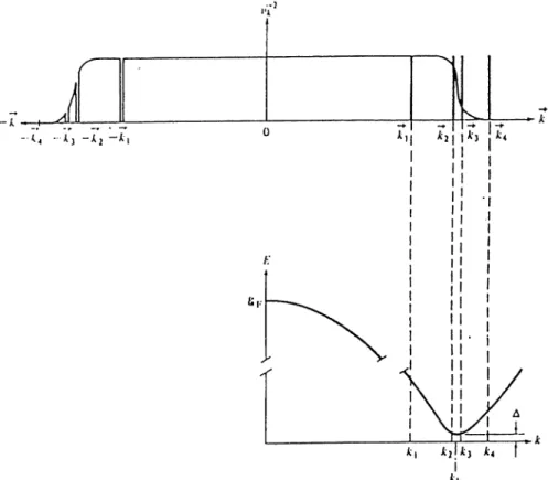
Therefore has a well-defined meaning (Fig. 2.13). The energy gap for

finite temperature is again given by

P but 2 E; k> /jc'T k' k'l> m (70)

CHAPTER 2. CONVENTIONAL SUPERCONDUCTIVITY 25

Figure 2.13: Excitation spectrum for BCS ground state

The upper plot shows the probability of occupation of states, the lower one is the

energy spectrum. is the energy of a single electron when it is excited from the

ground state by breaking of the pair k o ,—fco [2 6 ].

where is the expectation value of the quasi-particle occupation number.

Since these particles axe fermions is the Fermi-Dirac distribution function

1

fL· ~ _{exp(^Ej) + l} (71)

This result can be obtained more rigorously by minimizing the free energy. Then

ko k,ko 2 E r 2

k ^

Taking Vj in the approximate form

1 ^ dj ^7 ^ 2 + A2(0)

0) ^ Jo ^^2 + a2(0) 2 V^ ^ ^

N {0)V

(72)

(73)

In the weak coupling case, N (0)V C 1, remembering that ^ = l/ksT {ks is

temperature or from we have ksTc = A (0) = 2A(0) = 3.52¿bTc (74) (75) (76) This relation is a test for validity of the theory. It has been verified for many simple metals experimentally.

As we see within the simplifications of BCS theory, phonons enter to mea­

surable quantities only via the Debye frequency u>d. Through this dependence

BCS predicts the isotope effect correctly for simple metals

Tc cc a M-'>^ (77)

The reason for anomalies observed especially in transition metals is due to the breakdown of the two main approximations in the BCS theory

• is an Einstein frequency, exponent in the Tc expression (strength of

the electron phonon coupling) is independent of the phonon spectrum. • There axe no Coulomb effects, i.e., correlation interactions are neglected.

Thus the absence of isotope effect does not reject an electron phonon coupling mechanism while its presence is a sign for contribution of phonons to superconductivity.

Next, we describe the canonical transformation method. In a normal

metal the average < > is zero since phases axe random. But for the

superconductor we know that the Bloch states k and —k are both occupied

or they are both empty. In that case = < > is not zero. Then we

can write

CHAPTER 2. CONVENTIONAL SUPERCONDUCTIVITY 27

We have a large macroscopic system in equilibrium. Thus we expect that

quantities like fluctuate only in very small amounts around their av­

erage. This fact allows us to meike a simplification; in our calculations we neglect the terms quadratic in the expression in parentheses. Thus the Hamil­ tonian becomes

kj<7 kjP

We define

^ ic~ ^ ^ (^0)

P

which is analogous to the gap parameter in the BCS theory. Then

ky<7 k

After this step we apply a canonical transformation which is widely used in problems in which the Hamiltonian contains mixed terms. Our aim is to elim­ inate these mixed terms and obtain a Hamiltonian which contains constants and terms proportional to occupation numbers, i.e., ata. The transformation is

= ^I'Tko + ^aiitit .t

“-ifi = -^iτгo + «π¿^

(82)

where and are complex numbers with |ujgp + jujjP = 1. We can eas­

ily see that the new operators are also Fermi operators by evaluating the anticommutation relations.

Now we rewrite the Hamiltonian in terms of these new operators and

eliminate the mixed terms by choosing and vj^ properly.

H =

- l^iin(Tio7jfeo + 7|i7ifi) + 2|vjfp +

We have to eliminate TjfiTjfo coefficients of these two terms vanish when

= 0 (84)

which implies, along with the condition, |u^p + = 1

(

86

)

We see that the variational calculation and canonical transformation give the same answer.

Now the Hamiltonian is in the diagonal form and excitation energies be easily found ^ -^ H + ^ ¿ 4 ) + Ç k k where can

(

86

)

Thus we obtain the full spectrum at once. The first term is the condensation

energy. The quasi particles created by 7|’s are often called Bogoliubons. The

self consistency relation, in terms of the new operators, becomes

(88)

For the calculations at finite temperatures we note the fact that Bogoliubons obey the Fermi-Dirac statistics, therefore

< 1 “ 4'o^Po + TpiTitu > = 1

-exp PEt + 1

The gap equation, which is now temperature dependent, is given by №

A . - = - Ç % , ^ t a n h ^ | î

With the BCS approximation V^j^, = — F, we obtain

(89) (90) 1 1 ^ tanh /3Ea/2 V ~ 2 ^ Et k ^ (91)

CHAPTER 2. CONVENTIONAL SUPERCONDUCTIVITY 29

From this equation the temperature dependence of the gap can be found numerically. This result is a very important test of BCS theory since it is possible to obtain temperature dependence of the energy gap by electron tunneling experiments.

We can also find the thermodynamic quantities by calculating the entropy from

S = - 2 kB

E((l

%

For example by calculating the specific heat we can obtain one of the magic numbers of BCS

A C

Cn = 1.43 (93)

where Cn is the electronic specific heat in the normal state and A C =

Cs{Tc) — Cn(Tc) is the discontinuity at the critical temperature.

Another quantity which is directly observable in tunneling experiments is the density of states. We can find this function by a simple argument. We

can count the electrons either by quasi particle operators 'yj. or directly by

c|’s. Since both methods should give the same result we have

Ns{E)dE = NNiOd^ (94)

where Nn and Ns are the densities of states in the normal and superconduct­

ing states respectively and ^ is the energy of Bloch states. If the density of states in the normal state is a smooth function at the Fermi level we can as­

sume Nn( 0 — -^ (0) since superconductivity involves only a shell of thickness

o f which is four orders of magnitude smaller than the Fermi energy. In

fact we used this approximation in the BCS czilculations. Thus

Ns(E) _

[ T if e ; B > A

N{0) I 0

E < A

Figure 2.14 shows the plot of this function. Since the gap is very small in comparison to Fermi energy, band structure effects axe negligible.

By generalizing the Bogoliubov treinsformation it is also possible to handle spatial variations in inhomogeneous superconductors. In that case one uses

-E/A

Figure 2.14: Density of states in the superconducting phase

The vertical axis has been normalized with the normal state density of states. Note the square root singularity at the gap edge[32].

^ ( ^ i ) = S [7 n iiin (0 + 7 lT < (0 ]

n

where ^ t ’s create position eigenstates.

(95)

2.3.2

Strong Coupling Theory

When the electron-phonon coupling is strong BCS theory does not give an accurate description of superconducting properties. In such a case, when solving the gap equation, we should not only include attractive phonon in­ teraction but also the repulsive screened Coulomb interaction. This has been first done by Eliashberg.

We are not going to derive Eliashberg equations whose mathematical structure is much more complicated due to strong coupling nature o f the problem. The result is a frequency dependent gap equation

1 A' \ I (Ej'Re[—7 ] ^ ^ Z {uj) Jao V w' 2 -/•oo 1 1

X

J du}oa'^{uo)F{uo) { - — — ---^ + ~ --- T

CHAPTER 2. CONVENTIONAL SUPERCONDUCTIVITY 31

where phonon mass renormalization parameter Z is given by

[1 - Z ( .)] = j y R e l ^ ^ ]

yoo J

X /

du}oa^(iO o)F(uo

—

Jo to' + + Ct^o — oj' — + OJq — to

and the electron phonon coupling parameter ( replacing the parameter u =

N (0 )V in the BCS theory) is defined by

a ^ (u ;o )E M = d^P E \9vp·- <^P (98)

Here Ao is the gap at the gap edge, gppi^ is electron phonon coupling,

is the energy of the virtual dressed phonon, « is phonon polarization index,

vp is the Fermi velocity, Sp is the Fermi surface, and F((x>o) is the phonon

density of states

(99)

F (u}q) = E /

~

There is always a repulsion between electrons, although it is screened, /x* is a measure of Coulomb repulsion which is neglected in the BCS theory. We

may define a dimensionless measure p of the Coulomb interaction analogous

to 1/, and say u — p replaces u in the BCS theory. However, here we have

to carry out a renormalization procedure first done by Bogoliubov[33]. The problem is that while the Coulomb interaction propagates at the speed of light (or Fermi velocity for screened interaction), phonon interaction is not

faster than sound. Thus Bogoliubov showed that p should be replaced by p*

where

p* ~

1 + pln(Ep/%u>D)

In this way we obtain an equivalent instantaneous interaction.

H IG H T E M P E R A T U R E

SU P E R C O N D U C TO R S

Superconductivity was first observed in metals. In 1964 Cohen proposed that semiconducting type materials can also become super conductor [34]. This prediction was confirmed by the observation of superconductivity in the p -

type GeTe[35]. NhO and TiO were the first superconducting oxides (Ta­

ble 3.1). In these materials metallic properties survive in spite of the intro­ duction of oxygen. For the other materials since the interaction among the

metal atoms is too wealc metallic properties axe lost, e.g., they are not good

conductors above the superconducting transition temperature Tc. SrTiOz is

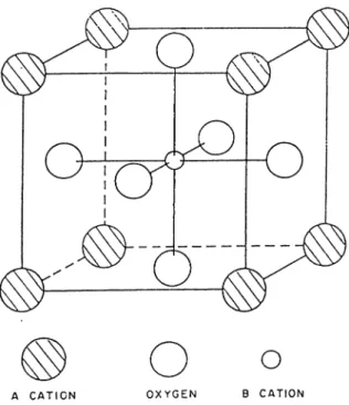
the first perovskite superconductor. Perovskites are cubic compounds of the

form A B O3 where A and B are cations. While A atoms sit on the corners of

the cube, R ’s axe located at the center.

The breakthrough in the superconductivity came with the discovery of copper oxides. Bednorz and Müller chose the transition metal oxides since these materials exhibit polaxonic effects indicating strong electron phonon interaction.

In this chapter we are going to review the physical properties of the new superconductors and make some remarks on their common properties.

CHAPTER 3. HIGH TEMPERATURE SUPERCONDUCTORS 33

Compound Tc Date discovered

TiO,NbO 1 K 1964 SrTiOz-x 0.7 K 1964 Bronzes A^WOz 6 K 1965 AxMoOz 4 K 1969 AxReOz 4 K 1969 AgrOsX 1 K 1966 LÍTÍ2O4 13 K 1974 Ba(Pb, Bi)Oz 13 K 1975 (La, Ba)2CuO^ 35 K 1986 Y Bü2CuzOj 95 K 1987 BilSr/Cu/O 22 K 1987

B ilSrJC alC ulO 90 K 1987

T llB alC alC u lO 122 K 1988

K jB a lB ilO 30 K 1988

N d lC elC u jO 24 K 1989

P blS vlY ¡C ulO 70 K 1988

Table 3.1: Oxide superconductors

Adapted from [11]

3.1

B a /P b /B i /O

BaPhi-xBixOz system is a perovskite superconductor over the range

x=0.0-0.30. The critical temperature increases when the Bi content is in­

creased and it reaches a maximum of 13 JiT for x=0.27. Further doping with Bi results in a superconductor to semiconductor trzinsition at a:=0.30.

According to crystallographic measurements the unit cell is orthorhom­

bic with a = 4.343A, b = 4.358A, and c = 4.333A[37j. BaPhOz has also a

perovskite structure with an orthorhombic cell of dimensions a = 6.024

A,

h = 6.065

A,

filled 0 — 2p bands BaPbOz shows metallic properties. Semiconducting char­

acter o f BaBiOz is not obvious since we expect that odd number of valence

Figure 3.1: Perovskite structure

This figure is taken from reference [36].

Figure 3.2: Phase diagram of BaPbi^xBixOs

Alternating valence of Bi causes the transition from metallic to semiconducting

phase[llj.

crystal structure is monoclinic with ^ = 90.2 and neutron diffraction experi­

ments indicate that there are two types of Bi in BaBiOz[^^]· These different

CHAPTER 3. HIGH TEMPERATURE SUPERCONDUCTORS 35

are expanded and compressed by 7% respectively and they are tilted by 10° relative to (110) axis . Each octahedra contain an even number of electrons and this configuration is consistent with the semiconducting char­

acter o f BaBiOz· The disproportionation ■(— > Bi^'^ -|- Bi’^'^ does not

imply that the real charges on Bi atoms are 3-|- or 5-f. Due to the covalent

nature of the bonds charges are much reduced. Muon experiments show that

BaBiOz is not an antiferromagnet. This result implies that Bi^'^ is not the correct configuration.

There are several experiments indicating that strong coupling of electrons to soft phonons plays an essential role in the high critical temperature of

BaPhx-xBixOz· In tunneling experiments a strong phonon structure has been observed[40]. On the other hand infrared measurements show that for

polycrystalline samples the gap ratio 2A/kTc is about 3.2 which is consistent

with the weak coupling BCS value 3.5[41]. It has been measured that the

penetration depth in BaPbi-xBixOz is about 5000 Aand the coherence length

is less than 100 A [40].

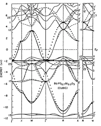
The electronic structure calculations show that the conduction band is

made of a-antibonding combinations of O — 2p and Bi(Pb) — 6s orbitals[42).

The LAPW energy bands can be well approximated by simple tight binding

models. The models involving three parameters with Eg, = —4.1 eV,E2p =

—l.QeVi Vspa = 2.2eV and five parameters which has additional entries E^p —

3.5eF, Vppa = 2.7eV and = —^Vpptr are also shown in Fig. 3.3.

The band is filled rigidly with increasing x. Strong coupling of conduc­

tion electrons to the lattice vibrations associated with the O bond stretching

displacements leads to a commensurate charge density wave (CDW)[39j.

3.2

L a /B a /C u /O

LaBaCuO is the first high Tc superconductor[10j. It has been shown

that the phase responsible for bulk superconductivity with Tc = 35/iT'is

La2-xBaxCu04 with x = 0.15(43]. At high temperatures _{La2-xMxCuOi-y}

(so called 2-1 -4 ) compound exhibits a body centered tetragonal lA/mmm