INNOVATIVE TREND ANALYSIS METHODOLOGY IN LOGARITHMIC AXIS
Sadık ALASHAN [email protected]
Bingöl University, Department of Civil Engineering, Campus, Bingöl, TURKEY
(Geliş/Received: 31.12.2019; Kabul/Accepted in Revised Form: 13.03.2020)
ABSTRACT: Future uncertainties of climate change cause people to worry, and therefore, in order to
reduce the associated risks, scientific research methodologies are improved continuously. For instance, temperature raises as a result of carbon content increase cause variations in hydro-meteorological data including evaporation, drought, precipitation, runoff, and flood. Along these lines, the most commonly used trend analysis methods are linear regression analysis, Mann-Kendall, sequential Mann-Kendall, Spearman’s Rho, and recently a new method referred to as innovative trend analysis (ITA), which does not require initial assumptions, normality, and independence in a data structure. The ITA method presents a great visual ability for trend identification in graphical forms in addition to qualitative and quantitative interpretations. In the original form of the ITA approach, scatter points are presented in the arithmetic scale, where changes of scatter points in small values may not be clearly distinguishable like big values for wide data ranges. In this study, the ITA method is used on arithmetic and logarithmic scales to calculate such differences in two sub-series. The suggested logarithmic scale methodology is referred to as proportional Şen innovative trend analysis (ITA_P). This method is used to determine percent trends for the annual, autumn, winter, spring and summer season rains in England. ITA_P is successful in determining trends in minimum values compared to the classical ITA.
Key Words: Innovative trend analysis, hydro-meteorological data, proportional innovative trend analysis, climate
change.
Logaritmik Ölçekte Yenilikçi Yönelim Çözümleme Yöntemi
ÖZ: Gelecekle ilgili belirsizlikler insanoğlunu endişelendirmekte ve olası riskleri azaltmak için bilimsel
araştırma yöntemleri sürekli geliştirilmektedir. Örneğin karbon salınımının artışıyla birlikte artan sıcaklıklar buharlaşma, yağış gibi iklim olaylarının değişimini artırarak akışlar üzerinde kuraklık ve taşkınlara neden olabilmektedir. Bu olaylar üzerindeki eğilimi belirlemek üzere Mann-Kendall, sıralı Mann-Kendall, Spearman rho ve son zamanlarda ortaya atılan Şen’in yenilikçi yönelim çözümleme (Şen_ITA) yöntemleri literatürde sıklıkla kullanılmaktadır. Bu yöntemlerden Şen_ITA yöntemi normallik ve bağımsız seri gibi başlangıç kabulleri gerektirmemektedir. Ayrıca niteliksel ve nicel yorumlamaları yanında grafiksel olarak görsel kabiliyeti yüksek bir yöntemdir. Şen_ITA yöntemi esasen aritmetik ölçekte kullanılır ve bu durum değişim katsayısı yüksek bir seri üzerinde minimum değerler üzerindeki eğilimin maksimum değerlerin yanında gözden kaçabilmesine neden olabilmektedir. Bu çalışmada, Şen_ITA yöntemi aritmetik ve logaritmik ölçekte kıyaslanmıştır. Önerilen yaklaşım, oransal Şen yenilikçi yönelim çözümleme yöntemi olarak adlandırılmıştır (ITA_P). Bu yaklaşım İngiltere’nin mevsimsel ve yıllık yağışları üzerindeki oransal eğilimleri belirlemek için kullanılmıştır. ITA_P yaklaşımının klasik Şen_ITA yöntemine göre bir seri üzerinde minimum değerlerdeki eğilimleri belirlemede daha başarılı olduğu belirlenmiştir.
Anahtar Kelimeler: Yenilikçi yönelim çözümlemesi, hidro-meteorolojik veri, oransal yenilikçi yönelim
1. INTRODUCTION
Climate change impacts hydro-meteorological events by incorporating an increasing trend component in temperature records and increasing or decreasing trends in precipitation, evaporation, flood and drought occurrences. The carbon level in the atmosphere affects the temperature, which impacts precipitation and evaporation, and they trigger floods and droughts according to the circumstances.
Mann-Kendall (MK), the sequential MK and Sen's slope estimator are well-known trend calculation methods and they are widely used in the literature (Büyükyıldız and Berktay, 2004; Kendall, 1975; Lin et al., 2008; Mann, 1945; Shahid, 2011; Vinet and Zhedanov, 2010). Recently, Şen innovative trend analysis (ITA) method is launched to determine the trend in a given time series (Şen 2012, 2014, 2017) and it has been used by many researchers. For instance, Elouissi et al. (2016) used ITA to investigate trends in monthly precipitation records from 28 meteorology stations in Algerian Macta watershed. Öztopal and Şen (2017) classified precipitation values as low, medium and high in the ITA graph and then determined trends in the precipitation values in different climate regions of Turkey. Some researchers compared the ITA and MK methods. For instance, Nourani et al. (2018) investigated trends in rainfall, streamflow, humidity and temperature records in Urmia lake basin, Iran and they stated that ITA indicated a good agreement with the MK method. Dabanlı et al. (2016) used MK and ITA methods to determine trends in hydro-meteorological variables such as relative humidity, temperature, runoff and precipitation at 8 stations in Ergene drainage basin, Turkey. They stated that MK does not give significant monotonic trends for the drainage basin while ITA provides verbal partial trend information (low, medium and high) in most of the stations.
Although the ITA method is based on a comparison of two half series, it is possible to work with more than two parts to detect even sudden shifts in a given time series. Deng et al. (2017) studied precipitation variability on Weizhou Island, the northern part of the South China Sea by using MK and ITA methods, where they divided the main record into three parts and found a non-homogenous temporal trend distribution. Sonali and Nagesh Kumar (2013) examined trends in Indian maximum and minimum temperatures with different data lengths using ITA and other well-known trend methods. Mohorji et al. (2017) applied the ITA to global monthly temperature values, first as two half series and then for various periods (10-year, 20-year, 30-year, 40-year, and 50-year). It was found that the increasing temperature at the global scale is about 0.75 °C. Güçlü (2018b, a) used ITA in half time series for possible determination of trend shifts by considering “increasing-increasing", "decreasing-increasing", "increasing-decreasing" and "decreasing-decreasing" cases.
ITA has a strong graphical visual ability to identify and interpret the trend possibility in a given time series. In the classical trend calculations, serial independence, homoscedasticity, and normal probability distribution assumptions must be satisfied. Şen_ITA method does not require these assumptions, and it is based on the comparison of the two ascendingly ordered halves from the original time series (Şen, 2017). In this method, the trend changes are documented quantitatively, where larger deviations may occur in the maximum values compared to the minimum values with respect to 1:1 (45º) no trend line. It is possible for the same trend in quantity to provide different percent changes in cases of daily or monthly records. The percent approach helps to expose trends on the minimum values.
The aim of this study is to adapt trends similar to the ITA method based on the logarithmic scale, which is referred to as proportional Şen innovative trend analysis (ITA_P). It is observed that similar trends in percent are at equal distance to 1: 1 (45º) no trend line for all series in logarithmic scale. In this way, small quantities and big proportions in the minimum values are easily observed by the ITA_P approach, which leads to better interpretations regardless of the data size.
2. MATERIAL AND METHOD
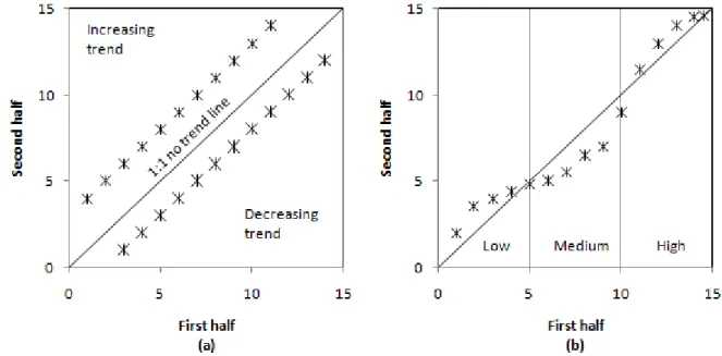
The Şen innovative trend analysis (ITA) is based on two sub-series comparison from a given parent hydro-meteorological time series. Each series is sorted in ascending order and the first
sub-series values are plotted on horizontal (X) against the second sub-sub-series on vertical (Y) axis leading to the scatter diagram graph as in Figure 1, where 1:1 (45°) line represents no trend straight-line. If the scatter points are above (under) the 1:1 line with approximately parallel positions then there is an increasing (decreasing) trend in the records, and this is referred to as a monotonic trend (Figure 1a). If the entire scatter points are not completely above, under or parallel to the 1:1 line then this is referred to as a non-monotonic trend and then the horizontal axis in the graph is divided into ranges such as low, medium, high, etc. (Figure 1b).
Figure 1. A graphical representation of the ITA method a) monotonic trend b) non-monotonic trend
(Alashan, 2018).
The basic equation for a trend in quantity related to the ITA method is given by Şen (2017) in the following expression.
s =
2(y̅−x̅)n
(1)
Here, s, 𝑦̅, 𝑥̅ and n are trend slope, arithmetic averages of the second and first sub-series and number of data, respectively. Positive (negative) slope values represent increasing (decreasing) trends, while there is no trend for zero slope value. Sometimes, although slope values are marginally bigger (smaller) than zero and in which case there is not any significant positive (negative) trend. For testing the trend significance, a 5% trend line is selected as the critical trend line. By selecting the critical trend value in percent, the critical trend line is determined without the need for assumptions such as normality and independence. Many critical trend lines such as 2%, 5%, 10%, and 20% are used in the ITA method in the literature (Ahmad et al., 2018; Cui et al., 2017; Kambezidis, 2018; Nisansala et al., 2019; Wu et al., 2017).
The difference at the i-th scatter point (a trend indicator) is defined as y𝑖− x𝑖, where 1 < i < n/2 (Wu and Qian, 2017). In the literature, the average trend indicator is divided into the mean of the first half series and the trend in percent (1
𝑛∑
𝑦𝑖−𝑥𝑖
𝑥̅ 𝑛
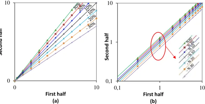
𝑖=1 ) is obtained. Figure 2 indicates the result of the ITA after the logarithmic transformation application on both axes (arithmetic and logarithmic) leading to the proportional Şen innovative trend analysis (ITA_P).
0
10
0
10
Se
con
d
ha
lf
First half
(a)
0,1
1
10
0,1
1
10
Seco
n
d
h
al
f
First half
(b)
Figure 2. Graphical representations of proportional innovative trend analysis a) arithmetic axis b)
logarithmic axis.
To avoid dependence on the mean of the first half series in trend calculations, the ratios of yi/xi lead to dimensionless changes (pi), according to the following expression.
𝑝𝑖=𝑦𝑥𝑖 𝑖 ⇒ 𝑝 = ( √∏ ( 𝑦𝑖 𝑥𝑖) 𝑛 𝑖=1 𝑛 ) (2)
The geometric mean change (p) is calculated for dimensionless values and α parameter is calculated by Eq. (3), which helps to determine a possible trend.
𝛼 = p − 1
(3)
If 𝑥̅ = 𝑦̅ then p=1 (scatter points fall over the 1:1 line) and α = 0 implies that there is no trend in the data. However, increasing (decreasing) trend exists in the case of p>1 and 𝑥̅ < 𝑦̅ (𝑝 < 1 𝑎𝑛𝑑 𝑥̅ > 𝑦̅). This last sentence implies also that if 𝛼 > 0 (𝛼 < 0) an increasing (decreasing) trend appears. Application of the logarithmic transformation to Eq.2 yields Eq.4, which implies a set of parallel straight-lines to the 1:1 no trend line according to different trend slopes (α) (Fig. 2b).
log(𝑝) =1 𝑛(log ( 𝑦1 𝑥1) + log ( 𝑦2 𝑥2) + ⋯ + log ( 𝑦𝑛 𝑥𝑛))
log(𝑝) =1
𝑛(log(𝑦1) − log (𝑥1) + log(𝑦2) − log (𝑥2) + ⋯ + log(𝑦𝑛) − log (𝑥𝑛)) (4)
3. APPLICATION AND STUDY AREA
The application of the ITA_P method is presented for monthly rain values from England. The country is approximately between 49.930 N to 55.8⁰ N latitudes and 5.72⁰ W to 1.77⁰ E longitudes. Some
of the important cities are selected as the study areas to observe the climate change impact on the country (Figure 3). The country has a maritime climate with frequent rain events. Annual mean rain values range from 600 mm to 3,000 mm. The eastern and western parts of the country are drier and warmer than the southern and northern parts. The western part has higher elevations that prevent the
humid air entrance from the Atlantic Ocean to the east. In addition, the high topography allows for cooling in the western parts and gives rise to intensive rain occurrences. Summer and spring seasons have relatively higher rain values than the autumn and winter seasons in the eastern parts, but in the western part, autumn and summer seasons have higher rain values compared to winter and spring seasons. Heathrow Camborne Eastbourne Lowestoft Sutton Bonington Sheffield Shawbury Whitby Newton Rigg Chivenor ENGLAND
Figure 3. Map of locations of the selected rain stations in the study area, England.
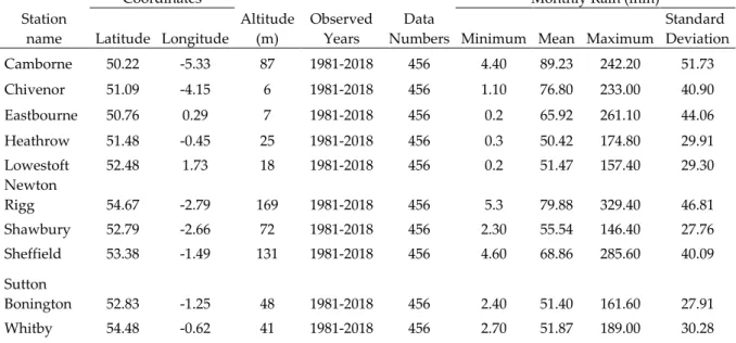
Statistical information about the rain stations is given in Table 1 with the minimum, average, maximum, and standard deviation. The rain database is provided by the Met Office which is the national meteorological service of the UK (https://www.metoffice.gov.uk /research/climate/maps-and-data /historic-station-/research/climate/maps-and-data). The homogeneity of the /research/climate/maps-and-database is checked by the Run homogeneity test proposed by Swed and Eisenhart (1943). The data of all stations used in the study provides a homogeneity condition of at least a 90% significance level. Newton Rigg station has the maximum altitude and the highest monthly rain values, while Lowestoft and Eastbourne stations are with the minimum rain. Shawbury and Camborne stations have minimum and maximum standard deviations, respectively.
Table 1. Statistical and geographic characteristics of the rain observation stations in the study area. Station name Coordinates Altitude (m) Observed Years Data Numbers Monthly Rain (mm)
Latitude Longitude Minimum Mean Maximum
Standard Deviation Camborne 50.22 -5.33 87 1981-2018 456 4.40 89.23 242.20 51.73 Chivenor 51.09 -4.15 6 1981-2018 456 1.10 76.80 233.00 40.90 Eastbourne 50.76 0.29 7 1981-2018 456 0.2 65.92 261.10 44.06 Heathrow 51.48 -0.45 25 1981-2018 456 0.3 50.42 174.80 29.91 Lowestoft 52.48 1.73 18 1981-2018 456 0.2 51.47 157.40 29.30 Newton Rigg 54.67 -2.79 169 1981-2018 456 5.3 79.88 329.40 46.81 Shawbury 52.79 -2.66 72 1981-2018 456 2.30 55.54 146.40 27.76 Sheffield 53.38 -1.49 131 1981-2018 456 4.60 68.86 285.60 40.09 Sutton Bonington 52.83 -1.25 48 1981-2018 456 2.40 51.40 161.60 27.91 Whitby 54.48 -0.62 41 1981-2018 456 2.70 51.87 189.00 30.28
The ITA and ITA_P methods are applied to the monthly rain records leading to graphs in Figure 4. It is obvious from these graphs that there are visual discrepancies between ITA and ITA_P methods. Although they have the same trends in quantity, the maximum (minimum) values have smaller (bigger) trends than the minimum (maximum) values. This leads to different visual trend evaluations between ITA and ITA_P scales. Camborne monthly rain records have no visually important trends according to the ITA (Figure 4), but there is an increasing trend in the minimum values according to the ITA_P method. According to ITA, there are increasing trends in Chivenor, Newton Rigg, Shawbury and Sheffield monthly maximum rain values, but the increasing trends in the ITA_P approach are seen at minimum values. Eastbourne, Lowestoft and Sutton Bonington monthly rain records have increasing trends in the ITA concerning the maximum values, but according to the ITA_P approach, there are decreasing trends in the minimum values. At Heathrow, no visual significant trend is seen according to ITA_P but there are increasing trends in the maximum values according to the ITA. There exists a continuously increasing trend on the ITA_P graph in maximum Whitby monthly rain values, and there is a monotonic increasing trend in the ITA graph in the maximum rain values.
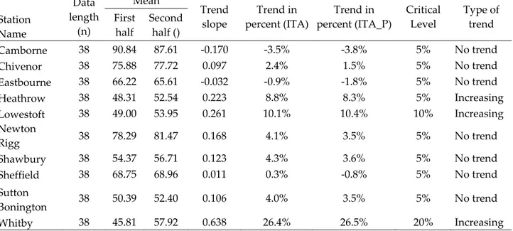
Monthly, annual and autumn, winter, spring and summer rain records are treated for trend identifications by means of ITA_P and ITA templates using Eqs. (1) - (4). The parameters in Table 2 are given only for the annual rain records. Trends in the ITA_P template are plotted only for the annual rain records in Figure 5. The green (dashed) lines represent the maximum and minimum changes in the ITA_P template for annual rain records and the black (straight) line is for no trend (1:1) line, the red (bold) line is for a trend in percent according to ITA_P method. Whitby has the largest increasing trend both in ITA and ITA_P methods. The annual rain records in Camborne have a slightly decreasing trend in ITA and the trend slope does not exceed the 5% risk level (Table 2). There is almost no trend in the ITA_P approach on Chivenor, Eastbourne, and Sheffield annual rain records (Figure 5). Newton Rigg, Shawbury and Sutton Bonington have small increasing trends in ITA_P. Heathrow, Lowestoft and Whitby station records have important increasing trends in the ITA_P template for annual rain records and the trend slope values exceed the 5%, 10% and 20% risk level.
Table 2. Trend results and statistical parameters for ITA and ITA_P methods in annual rain values.
Station Name Data length (n) Mean Trend slope Trend in percent (ITA) Trend in percent (ITA_P) Critical Level Type of trend First half Second half () Camborne 38 90.84 87.61 -0.170 -3.5% -3.8% 5% No trend Chivenor 38 75.88 77.72 0.097 2.4% 1.5% 5% No trend Eastbourne 38 66.22 65.61 -0.032 -0.9% -1.8% 5% No trend Heathrow 38 48.31 52.54 0.223 8.8% 8.3% 5% Increasing Lowestoft 38 49.00 53.95 0.261 10.1% 10.4% 10% Increasing Newton Rigg 38 78.29 81.47 0.168 4.1% 3.5% 5% No trend Shawbury 38 54.37 56.71 0.123 4.3% 3.6% 5% No trend Sheffield 38 68.75 68.96 0.011 0.3% -0.8% 5% No trend Sutton Bonington 38 50.39 52.40 0.106 4.0% 3.5% 5% No trend Whitby 38 45.81 57.92 0.638 26.4% 26.5% 20% Increasing
Table 3 presents trend both in ITA and ITA_P templates for annual, autumn, winter, spring and summer seasons. Trends slope in quantity changes from -0.170 mm/year (Camborne) to 0.638 mm/year (Whitby) for annual; from 0.376 mm/year (Eastbourne) to 0.875 mm/year (Whitby) for autumn; from -0.468 mm/year (Camborne) to 0.687 mm/year (Newton Rigg) for winter; from -0.495 mm/year (Newton Rigg) to 0.245 mm/year (Whitby) for spring and from 0.079 mm/year (Eastbourne) to 0.807 (Newton Rigg) mm/year for summer rain values.
Trends in ITA_P change from -3.85% per duration (Camborne) to 26.50% (Whitby) for annual rain values; from -12.49% (Eastbourne) to 33.21% (Whitby) for autumn; from -8.19% (Camborne) to 28.90% (Newton Rigg) for winter; from -12.08% (Newton Rigg) to 12.41% (Whitby) for spring and from 10.42% (Eastbourne) to 30.95% (Whitby) for summer rain values.
After the comparison between ITA and ITA_P methods according to trends in percent, Sheffield (Whitby) seems to have the highest decreasing (increasing) trend in percent for winter rain values in the ITA, while Camborne (Whitby) has the highest decreasing (increasing) trend according to ITA_P.
Figure5. Graphical representations of the trends in the ITA_P template for annual rain records in
Table3. Trend results in quantity and percent in rain values by ITA and ITA_P methods. Station name Camborne Chivenor Eastbourne Heathrow Lowestoft Newton
Rigg Shawbury Sheffield
Sutton Bonington Whitby Mo n th ly s (mm/year) -0.0141 0.0080 -0.0027 0.0186 0.0217 0.0140 0.0103 0.0009 0.0089 0.0531 CL (±) 5.0% 5.0% 5.0% 5.0% 10.0% 5.0% 5.0% 5.0% 5.0% 20.0% ITA (%) -3.55% 2.42% -0.92% 8.77% 10.11% 4.07% 4.31% 0.32% 4.01% 26.44% Decision ITA No trend No trend No trend Increasing Increasing No trend No trend No trend No trend Increasing
ITA_P (%) 1.97% 5.10% 1.29% 11.69% 9.34% 6.17% 6.97% 3.73% 6.11% 27.49% Decision
ITA_P No trend Increasing No trend Increasing Increasing Increasing Increasing No trend Increasing Increasing
A n n ual s (mm/year) -0.170 0.097 -0.032 0.223 0.261 0.168 0.123 0.011 0.106 0.638 CL (±) 5.0% 5.0% 5.0% 5.0% 10.0% 5.0% 5.0% 5.0% 5.0% 20.0% ITA (%) -3.55% 2.42% -0.92% 8.77% 10.11% 4.07% 4.31% 0.32% 4.01% 26.44% Decision ITA No trend No trend No trend Increasing Increasing No trend No trend No trend No trend Increasing
ITA_P (%) -3.85% 1.48% -1.81% 8.34% 10.38% 3.49% 3.57% -0.79% 3.51% 26.50% Decision
ITA_P No trend No trend No trend Increasing Increasing No trend No trend No trend No trend Increasing
A u tu m n s (mm/year) -0.193 -0.153 -0.376 0.206 0.331 0.227 0.067 0.033 -0.096 0.875 CL (±) 5.0% 5.0% 5.0% 5.0% 10.0% 5.0% 5.0% 5.0% 5.0% 20.0% ITA (%) -3.44% -3.07% -8.05% 7.06% 11.42% 4.68% 2.10% 0.86% -3.35% 33.86% Decision ITA No trend No trend Decreasing Increasing Increasing No trend No trend No trend No trend Increasing
ITA_P (%) -4.91% -5.60% -12.94% 10.10% 13.73% 5.30% 0.82% -1.07% -3.48% 33.21% Decision
ITA_P No trend Decreasing Decreasing Increasing Increasing Increasing No trend No trend No trend Increasing
Wint
er
s (mm/year) -0.468 0.047 0.383 0.363 0.291 0.132 -0.053 -0.388 -0.126 0.687
CL (±) 5.0% 5.0% 5.0% 10.0% 10.0% 5.0% 5.0% 5.0% 5.0% 20.0%
ITA (%) -7.48% 1.02% 9.69% 14.18% 11.69% 2.65% -1.83% -9.08% -4.77% 27.65% Decision ITA Decreasing No trend Increasing Increasing Increasing No trend No trend Decreasing No trend Increasing
ITA_P (%) -8.19% 2.87% 12.58% 16.96% 15.02% 2.10% -0.38% -8.02% -3.36% 28.90% Decision
ITA_P Decreasing No trend Increasing Increasing Increasing No trend No trend Decreasing No trend Increasing
Spr
ing
s (mm/year) -0.411 -0.027 -0.214 0.041 0.079 -0.495 -0.015 -0.157 0.071 0.245
CL (±) 5.0% 5.0% 5.0% 5.0% 5.0% 10.0% 5.0% 5.0% 5.0% 10.0%
ITA (%) -10.42% -0.88% -7.82% 1.77% 3.44% -14.51% -0.57% -4.76% 2.99% 11.54% Decision ITA Decreasing No trend Decreasing No trend No trend Decreasing No trend No trend No trend Increasing
ITA_P (%) -8.29% 0.75% -7.94% 2.34% -0.93% -12.08% -1.13% -4.06% 5.15% 12.41% Decision
ITA_P Decreasing No trend Decreasing No trend No trend Decreasing No trend No trend Increasing Increasing
Sum m er s (mm/year) 0.393 0.519 0.079 0.282 0.342 0.807 0.494 0.558 0.576 0.743 CL (±) 10.0% 10.0% 5.0% 10.0% 10.0% 20.0% 10.0% 10.0% 20.0% 20.0% ITA (%) 11.89% 15.42% 3.04% 11.89% 12.99% 24.99% 18.21% 18.00% 21.23% 30.33% Decision ITA Increasing Increasing No trend Increasing Increasing Increasing Increasing Increasing Increasing Increasing
ITA_P (%) 15.80% 16.21% 10.42% 16.54% 14.43% 25.94% 23.04% 19.13% 28.16% 30.95% Decision
ITA_P Increasing Increasing Increasing Increasing Increasing Increasing Increasing Increasing Increasing Increasing
Figure 6 shows the regional distribution of trends in the study area. Camborne city has decreasing trends for winter and spring rain values and has an increasing trend for the summer season. Chivenor has a decreasing trend for winter rain values and an increasing trend for summer rain values.
∆ 𝐼𝑛𝑐𝑟𝑒𝑎𝑠𝑖𝑛𝑔 𝑡𝑟𝑒𝑛𝑑 ∇ 𝐷𝑒𝑐𝑟𝑒𝑎𝑠𝑖𝑛𝑔 𝑡𝑟𝑒𝑛𝑑 𝑜 𝑁𝑜 𝑡𝑟𝑒𝑛𝑑
Figure6. ITA and ITA_P trend test results for all season’s rain records in the England map
Eastbourne has increasing trends for the winter and summer seasons and has decreasing trends for autumn and spring seasons. There are increasing trends for annual, autumn, winter and summer rain values in Heathrow. Lowestoft has increasing trends for all seasons excluding spring season and there is
no trend for the spring season. Sutton Bonington has increasing trends for all seasons excluding spring and there is no trend for the spring season. There is an increasing trend for the summer season in Shawbury. Sheffield has a decreasing trend for winter rain values and an increasing trend for the summer season. Whitby has increasing trends for all seasons. Newton Rigg has increasing trends for autumn and winter seasons but a decreasing trend for the spring season.
4. RESULTS AND DISCUSSIONS
The ITA method has great visual ability. Although it determines trends in quality and quantity but may give rise to overlook the trends in minimum values in wide-range axes graphs. Alternatively, the proportional Şen Innovative Trend Method (ITA_P) is suggested in this paper for more refined trend identifications in logarithmic scales. Zero and negative values cannot be represented by a logarithmic scale. Hydro-meteorological records (wind, rain, flow, flood, and drought, etc.) excluding temperature values as Celsius are not measured by negative values. If temperatures values are converted from Celsius (°) to Fahrenheit (F), they can be used on a logarithmic scale by the ITA_P method. In engineering studies, very small values can be accepted approximately zero with certain error (5% or 10%) and these values can be plotted on a logarithmic scale. Also, changes are determined as a rate (second-half value/first half value) in ITA_P and these proportions are positive even though measurement values are negative. The applications of the ITA and ITA_P methodologies are performed for monthly, annual, autumn, winter, spring and summer seasons rains records in England. While many researchers (Fowler and Kilsby, 2003; Osborn and Hulme, 2002) have reported decreasing trends in summer rains in the UK, there is an upward trend for summer rains in all regions of England. In relation to this situation, de Leeuw et al. (2016) states that the trend reversed in summer rainfall after 2007. Also, Whitby has a serious upward trend in all seasons. Annual rains give increasing trends for only 3 stations, and no trends are seen at other stations. In other seasons except for summer, the increasing and decreasing trends are seen together over England.
REFERENCES
Ahmad, I., Zhang, F., Tayyab, M., Anjum, M. N., Zaman, M., Liu, J., Farid, H. U., and Saddique, Q. (2018). “Spatiotemporal analysis of precipitation variability in annual, seasonal and extreme values over upper Indus River basin.” Atmospheric Research, 213, 346–360.
Alashan, S. (2018). “An improved version of innovative trend analyses.” Arabian Journal of Geosciences, 11(3), 50.
Büyükyıldız, M., and Berktay, A. (2004). “Parametrik Olmayan Testler Kullanilarak Sakarya Havzasi Yağişlarinin Trend Analizi.” Selçuk Üniversitesi Mühendislik, Bilim Ve Teknoloji Dergisi, 19(2), 23– 38.
Cui, L., Wang, L., Lai, Z., Tian, Q., Liu, W., and Li, J. (2017). “Innovative trend analysis of annual and seasonal air temperature and rainfall in the Yangtze River Basin, China during 1960–2015.” Journal of Atmospheric and Solar-Terrestrial Physics.
Dabanlı, İ., Şen, Z., Yeleğen, M. Ö., Şişman, E., Selek, B., and Güçlü, Y. S. (2016). “Trend Assessment by the Innovative-Şen Method.” Water Resources Management.
Deng, S., Li, M., Sun, H., Chen, Y., Qu, L., and Zhang, X. (2017). “Exploring temporal and spatial variability of precipitation of Weizhou Island, South China Sea.” Journal of Hydrology: Regional Studies, 9, 183–198.
Elouissi, A., Şen, Z., and Habi, M. (2016). “Algerian rainfall innovative trend analysis and its implications to Macta watershed.” Arabian Journal of Geosciences, 9(4).
Fowler, H. J., and Kilsby, C. G. (2003). “Implications of changes in seasonal and annual extreme rainfall.” Geophysical Research Letters.
Güçlü, Y. S. (2018a). “Alternative Trend Analysis: Half Time Series Methodology.” Water Resources Management.
Güçlü, Y. S. (2018b). “Multiple Şen-innovative trend analyses and partial Mann-Kendall test.” Journal of Hydrology, Elsevier, 566, 685–704.
Kambezidis, H. D. (2018). “The solar radiation climate of Athens: Variations and tendencies in the period 1992–2017, the brightening era.” Solar Energy.
Kendall, M. G. (1975). “Rank Correlation Methods, Charles Griffin, London (1975).” Google Scholar.de Leeuw, J., Methven, J., and Blackburn, M. (2016). “Variability and trends in England and Wales precipitation.” International Journal of Climatology.
Lin, X., Zhang, Y., Yao, Z., Gong, T., Wang, H., Chu, D., Liu, L., and Zhang, F. (2008). “The trend on runoff variations in the Lhasa River Basin.” Journal of Geographical Sciences, 18(1), 95–106. Mann, H. B. (1945). “Nonparametric Tests Against Trend.” Econometrica, 13(3), 245.
Mohorji, A. M., Şen, Z., and Almazroui, M. (2017). “Trend Analyses Revision and Global Monthly Temperature Innovative Multi-Duration Analysis.” Earth Systems and Environment, 1(1), 9. Nisansala, W. D. S., Abeysingha, N. S., Islam, A., and Bandara, A. M. K. R. (2019). “Recent rainfall trend
over Sri Lanka (1987–2017).” International Journal of Climatology.
Nourani, V., Danandeh Mehr, A., and Azad, N. (2018). “Trend analysis of hydroclimatological variables in Urmia lake basin using hybrid wavelet Mann--Kendall and Şen tests.” Environmental Earth Sciences, 77(5), 207.
Osborn, T. J., and Hulme, M. (2002). “Evidence for trends in heavy rainfall events over the UK.” Philosophical Transactions of the Royal Society A: Mathematical, Physical and Engineering Sciences. Öztopal, A., and Şen, Z. (2017). “Innovative Trend Methodology Applications to Precipitation Records in
Turkey.” Water Resources Management, 31(3), 727–737.
Shahid, S. (2011). “Trends in extreme rainfall events of Bangladesh.” Theoretical and Applied Climatology, 104(3–4), 489–499.
Sonali, P., and Nagesh Kumar, D. (2013). “Review of trend detection methods and their application to detect temperature changes in India.” Journal of Hydrology, 476, 212–227.
Swed, F. S., and Eisenhart, C. (1943). “Tables for Testing Randomness of Grouping in a Sequence of Alternatives.” The Annals of Mathematical Statistics.
Şen, Z. (2012). “Innovative Trend Analysis Methodology.” Journal of Hydrologic Engineering, 17(9), 1042– 1046.
Şen, Z. (2014). “Trend Identification Simulation and Application.” Journal of Hydrologic Engineering, American Society of Civil Engineers, 19(3), 635–642.
Şen, Z. (2017). “Innovative trend significance test and applications.” Theoretical and Applied Climatology, 127(3–4), 939–947.
Vinet, L., and Zhedanov, A. (2010). “A ‘missing’ family of classical orthogonal polynomials.” Journal of the American Statistical Association, 63(324), 1379–1389.
Wu, H., Li, X., and Qian, H. (2017). “Detection of anomalies and changes of rainfall in the Yellow River Basin, China, through two graphical methods.” Water (Switzerland).
Wu, H., and Qian, H. (2017). “Innovative trend analysis of annual and seasonal rainfall and extreme values in Shaanxi, China, since the 1950s.” International Journal of Climatology, 37(5), 2582–2592.