Received December 25, 2020, accepted January 4, 2021, date of publication January 8, 2021, date of current version January 20, 2021. Digital Object Identifier 10.1109/ACCESS.2021.3049896
LSTM and Filter Based Comparison Analysis for
Indoor Global Localization in UAVs
ABDULLAH YUSEFI 1,2, AKIF DURDU 2,3, MUHAMMET FATIH ASLAN2,4,
AND CEMIL SUNGUR2,3
1Computer Engineering, Konya Technical University, 42250 Konya, Turkey 2Robotics Automation Control Laboratory (RAC-LAB), TR-42075 Konya, Turkey 3Electrical and Electronics Engineering, Konya Technical University, 42250 Konya, Turkey 4Electrical and Electronics Engineering, Karamanoglu Mehmetbey University, 70100 Karaman, Turkey Corresponding author: Abdullah Yusefi ([email protected])
ABSTRACT Deep learning (DL) based localization and Simultaneous Localization and Mapping (SLAM) has recently gained considerable attention demonstrating remarkable results. Instead of constructing hand-crafted algorithms through geometric theories, DL based solutions provide a data-driven solution to the problem. Taking advantage of large amounts of training data and computing capacity, these approaches are increasingly developing into a new field that offers accurate and robust localization systems. In this work, the problem of global localization for unmanned aerial vehicles (UAVs) is analyzed by proposing a sequential, end-to-end, and multimodal deep neural network based monocular visual-inertial localization framework. More specifically, the proposed neural network architecture is three-fold; a visual feature extractor convNet network, a small IMU integrator bi-directional long short-term memory (LSTM), and a global pose regressor bi-directional LSTM network for pose estimation. In addition, by fusing the traditional IMU filtering methods instead of LSTM with the convNet, a more time-efficient deep pose estimation framework is presented. It is worth pointing out that the focus in this study is to evaluate the precision and efficiency of visual-inertial (VI) based localization approaches concerning indoor scenarios. The proposed deep global localization is compared with the various state-of-the-art algorithms on indoor UAV datasets, simulation environments and real-world drone experiments in terms of accuracy and time-efficiency. In addition, the comparison of IMU-LSTM and IMU-Filter based pose estimators is also provided by a detailed analysis. Experimental results show that the proposed filter-based approach combined with a DL approach has promising performance in terms of accuracy and time efficiency in indoor localization of UAVs.
INDEX TERMS Global localization, pose estimation, recurrent convolutional neural networks, bi-directional LSTM, VIO.
I. INTRODUCTION
Unmanned Aerial Vehicles (UAVs) are capable of complet-ing a wide range of applications, such as trackcomplet-ing, facility inspection, supply distribution, mapping, etc. At the same time, a precise estimation of the UAVs pose is essential to ensure a high level of safety in autonomous operations. The capability of an autonomous agent to accurately estimate its pose is known as Localization in mobile robotics [1], [2] and global localization is its ability to retrieve its global pose in a known scene with prior knowledge [3].
The associate editor coordinating the review of this manuscript and approving it for publication was Aysegul Ucar .
Among several localization methods available, the com-munity has drawn considerable attention to camera-based solutions [4] due to their low-cost, portability, simple hard-ware set-up and ability to give rich information about the scene. The technique is called Visual Odometry (VO) [5], [6] when cameras are used to calculate odometry. With the advances in computer vision, VO has been studied in recent years with excellent results [5], [7]–[10]. For instance, the ORB-SLAM [11] and the DSO [9], two members of feature-based [11]–[13] and direct-based VO [9], [14], [15] methods, respectively, achieve real-time output on CPUs and are both extremely accurate in the normal large-scale environment.
A typical VO approach generally includes acquisition of images, calibrating camera and correcting image, detecting features, tracking features for optical flow, removing out-lines and estimating motion by using obtained optical flow. More advanced methods for VO and SLAM might include some optimizing, bundle adjustment and loop closure. Even though some advanced methods which utilize this workflow demonstrate outstanding results with regard to robustness and precision, they are typically hand-engineered, and for the best performance, have to be manually fine tuned carefully for every module in the pipeline. In addition, a full scale needs to be approximated for the monocular camera based localization by using additional or previous sensor informa-tion, which makes it more susceptible to drift and complex situations. Furthermore,monocular VO suffers from the diffi-culty in initialization for slow motions [11], and the tracking tends to fail miserably in unconstrained environments with featureless places, low-light conditions, fast motions, pres-ence of dynamic objects in the scene or other adverse factor [16] such as the rolling shutter effect [17], [18] and camera occlusion [19], [20].
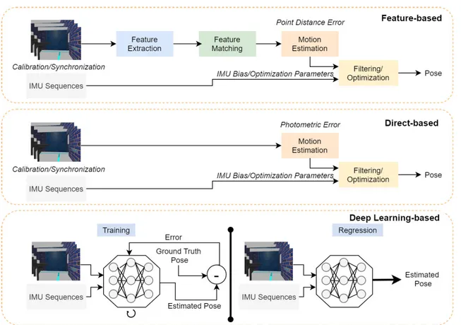
Deep learning (DL) has recently dominated several visual related areas with significant improvements, including clas-sification [22], object detection [21], semantic segmentation [23] and more. Following DL, the emergence of convo-lutional neural networks (CNN) created alternate solutions to VO which demonstrated both precise and robust com-petitive performance [24]–[26]. The advent of CNN’s have made VO issues more appealing by training DL networks to learn feature extraction from data instead of using fea-tures extracted by hand-engineered algorithms and descrip-tors [24], [25]. However, depending only on the learned visual features restricts the pose estimation to best operate in the learned environment causing overfitting and seriously prevents it from generalization to unseen or new environ-ments. Therefore, the use of CNNs only are not adequate for DL-based localization and It is important for the deep neural networks to carry out sequential learning. The comparison of the pipeline for VO based on features, density and DL is shown in Figure 1.
In this work, the problem of global localization is dis-cussed by proposing a sequential, end-to-end and multi-modal deep neural network based monocular visual-inertial global localization framework. In addition, this formulation is more extended by providing additional benchmark infor-mation by further comparison with traditional filter based inertial measurement unit (IMU) data versus DL based long short-term memory (LSTM). It is worth pointing out that the focus in this study is to evaluate the precision and effi-ciency of visual-inertial (VI) based localization approaches with respect to indoor scenarios, by comparing visual iner-tial odometry (VIO) algorithms, including direct-based and feature-based and, in particular, data-driven-based algo-rithms (DL approaches). The major contribution in particular are:
• We demonstrate that using DL, it is possible to tackle
the monocular VIO problem by a novel framework that can directly estimate the position of the camera with-out having to know the absolute scale and parameters beforehand.
• We propose a multimodal RNN architecture that allows
the DL-based global localization to be generalized to unseen and new environments via the visual and tem-poral feature extraction trained on CNN and LSTM. It consists of one CNN model and two bidirectional LSTM models for extracting visual features from raw camera frames. The first model is used by the IMU sensor to synchronize the arrays of acceleration and angular velocity with camera frame sequences. The sec-ond LSTM is used to derive the temporal characteristics derived from features fusion of the previous two models.
• As an alternative to the smaller LSTM model, we will
then incorporate filter-based IMU processing methods (Mahony, Madgwick, Extended Kalman Filter (EKF), Unscented Kalman Filter (UKF)) and compare their performances on our data-driven VIO.
• Finally, using the publicly available EuRoC MAV
dataset and simulation environment, we evaluate the efficiency of our VIO system and compare it to VIO baseline algorithms. The findings show that our approach is significantly superior compared to the state-of-the-art localization of UAVs, enhancing the accuracy. The remainder of this paper is structured as follows: Section 2 includes a summary of literature on motion esti-mation, beginning with traditional methods, discussing visual based SLAM and eventually highlighting some latest stud-ies on DL. In Section 3, followed by experimental results in Section 4, the end-to-end monocular VIO algorithm and its baseline methods for processing IMU measurements are described. Finally, the discussion, conclusion and poten-tial directions for future investigations are provided in sec-tions 5 and 6.
II. RELATED WORKS
Numerous methods have been suggested for pose estima-tion in the literature. Early work on the monocular VO/VIO is reviewed in this section, discussing some of the tech-niques and frameworks developed to date to tackle this issue. In terms of the methodology and system implemented, there are primarily two types of VO/VIOs: traditional methods which are based on geometry and data-driven methods which are based on learning.
A. TRADITIONAL METHODS
VO is performed by evaluating instant camera motions over consecutive frames, and accumulating them to obtain the relative trajectory on a global reference frame. Generally, tra-ditional VO/VIO methods are divided into three distinct types in the literature: direct-based, feature-based and hybrid-based approaches.
FIGURE 1. Feature-based, Direct-based and DL-based VO workflow.
Feature-based methods use a range of feature detectors such as SURF (Speeded Up Robust Features) [27], FAST (Features from Accelerated Segment Test) [28], SIFT (Scale-Invariant Feature Transform) [29], ORB (Oriented FAST and Rotated BRIEF) [30] and Harris and Stephens [31] to detect key points. These features are then tracked in the next sequential frame using a key point tracker resulting in optical flow, the most common of which is the KLT tracker [32], [33]. As suggested by Nister [34], the camera-parameters can then be used to estimate the ego-motion. A broad variety of work has been carried out on various techniques of VO/VIO, including different camera setups [35], [36], configuration of camera parameters and bundle adjustment methods to optimize the pose [37]. In addition, Study in [38] pro-posed a 1-point motion evaluation algorithm in 2011 that leveraged the physical limitations to reduce the complexity of the model. Kitt el al.’s other popular work, LIBVISO, an open source VO evaluation library, has been published, capable of estimating 6-DoF poses both in mono and stereo camera configurations [39]. It is also an invaluable technique to combine visual information with other complementary sensorization [40], such as GPS or IMU data, as estimated computation generally becomes more robust. Kasik et al. sug-gested another interesting method by using non-overlapping cameras to mimic a stereo camera system [41]. Here, the assumption is the monocular VO is estimated from each camera and the stereo restriction is later enforced.
Direct-based methods rely heavily on the intensity of all or parts of image pixels. For estimating the motion between two images they utilize the photometric error optimization. Such methods, however, include the assumption of flatness (e.g. homography). Early direct SLAM approaches such as [42] and [43] use filtering algorithms for SFM, while non-linear minimum square estimates have been used for [44] and [45]. Other methods, such as DTAM [46], evaluate the dense depth map of each keyframe to align the entire image to locate the camera pose. This is done by optimizing the global energy function. Since this approach is computation-intensive, a strong parallelization of the GPU is required. The method referred to in [15] is proposed to alleviate this high computational requirement. The LSD-SLAM algorithm has also recently been introduced in order to achieve fast direct monocular SLAM [14]. More recently, the photometric defect is optimized in the form of a sparse bundle modification in a direct approach proposed in [9]. It removes the need for geometric priors usually encoded with features by using all picture points, also in the lesser textured areas, to estimate egomotion.
Hybrid Methods combine both feature-based and direct-based methods in order to further improve algorithmic robustness to complex unstructured scenarios. Recently, they are increasingly gaining more favour for the monocular VO/VIO [15]. In [47], Scaramuzza et al. proposed a hybrid approach to use feature-based method as translation estimator
and dense-based method as rotation estimator in plane sur-face. Study in [10] proposed SVO, in which localizations are optimized by reducing the reprojection defects of feature adjustment. In combination with feature-based translation factor and then refined via a Kalman filter, study in [48] pro-poses the dense ego-motion estimation technique. This work was then expanded to a completely dense stereo ego-motion probabilistic system which increases the robustness to more challenging environments [49].
B. DATA-DRIVEN METHODS
Although DL is only relatively recently applied in the field of VO/VIO methods, much research has been devoted to optimizing its field potential. In this respect, it can be catego-rized as an ego-motion estimation that calculates the relative motion between two consecutive images and the global local-ization that concerns the global pose estimation of a robot in a specified, prior-knowledge environment.
Ego-motion estimation is to predict the gradual motion of a robot using sequential camera images. Konda and Memise-vic [50] used a classification technique to pose estimation in one of these earlier methods, using convNet with the softmax layer to infer the ego-motion between two camera frames labeled with discrete changes of direction and velocity. In another approach suggested by Nicholai et al. [51], image and LiDAR data are combined to estimate the ego-motion between two inputs of the camera. They extract the point cloud from the 2D image and input this data into a neural network to obtain trajectory. The study in [52] used CNN to extract visual features from dense optical flows and to esti-mate sequential motion based on these visual characteristics. However, these approaches still lacked the end-to-end ability of pose estimation from images.
In order to tackle this issue, A Siamese and recurrent neural network (RNN) based architecture was developed by Mohanty et al. [53] to estimate the robot pose through a layer of L2 loss with equivalent weights. In a related paper, Melekhov et al. [54] apply a weighting concept to the loss balance of pose parameters that improve the pose regression. In addition, they have a framework with a pooling layer that makes their method more robust to various image quali-ties. Saputra et al. [55] includes geometrical loss restrictions in order to increase consistency between multiple poses. In addition, Xue et al. [56] implemented a memory module for storing global information and a refinement module for enhancing pose estimation. However, all of the ego-motion approaches referred to above are supervised methods and need ground truth labels of poses to train. At this time, it is usually challenging and costly to acquire ground truth labels in practice, which makes the number of currently labeled training datasets somewhat limited.
In order to deal with these limitations, there has been a growing interest in exploring unsupervised learning of VO. Unsupervised methods can learn from unlabeled data, and therefore save human labeling effort and have a greater capac-ity to adapt and generalize in unseen environments, where no
labeled data are present. This is achieved in a self-supervised architecture that uses view synthesis technique to learn both depth and camera relative pose from video sequences [57]. However, this work suffers from scale ambiguity and sensi-tivity to camera occlusions. In order to address these issues, a number of works extended this framework to improve the performance [58]–[66].
Considering that IMU is a low-cost, power efficient and widely deployed sensor, it has opened its way in DL based VOs. VINet [24] was the first work to articulate the sequential learning issue of VIO and suggest a profound network archi-tecture for end-to-end VIO. Chen et al. [67] suggested a sen-sor fusion architecture that selectively learns context aware representations for VIO. VIOLearner [68] obtains motion estimations from raw inertial data without the inertial IMU intrinsic parameters or the extrinsic calibration between IMU and camera. In addition, DeepVIO [69] integrates IMU and stereo camera data and is trained with a dedicated loss to reconstruct relative poses on a global scale.
Global Localization is the extraction of a robot’s absolute position in a known environment. The first work that used convNets as an absolute camera pose regressor was PoseNet [25] that worked in an end-to-end manner. This was then expanded in [70] by using multi-view geometry to improve PoseNet efficiency. Melekhov et al. [71] used ResNet34 in the original pipeline and Walch et al. utilized LSTM for dimen-sionality reduction [72] and some works have used synthetic target image generation to augment training data [73]–[75]. Hunag et al. [76] and Wang et al. [77] have shown that self-attention modules can greatly enhance localization accu-racy and instruct the network in the complex environment to ignore distracting information from foreground objects. Clark et al. [26] integrated temporal constraints in addition to spatial constraints to support temporal connections between images. In addition, GPS information was used by [78] to improve the accuracy of motion between the estimated poses. Moreover, [79] and [80] joined global localization and rel-ative pose estimation networks. Finally, [81] and [82] used more information constraints such as semantics and com-bining information with pose regressor networks to achieve higher pose estimations.
Towards the DL based global localization approaches pre-sented above, we propose a joint trainable multimodal frame-work that simultaneously estimates the 6 DoF global pose in an end-to-end manner. By jointly learning both features from IMU measurements and camera frames and applying two bi-directional LSTMs, our method is robust to con-text mutation in the environment by utilizing past sensor measurements, thereby merging the benefits of both LSTM and ConvNet methods. Moreover, by integrating the tradi-tional IMU measurement filtering methods instead of LSTM with the CNNs we demonstrate a more time-efficient deep pose estimation framework. Additionally, a comparison of these methods is done on publicly available EuRoC dataset and simulation environment to VIO benchmark algorithms. Experimental results show that the proposed filter-based
approach combined with a DL approach has promising per-formance in terms of accuracy and time efficiency in indoor localization of UAVs.
III. DEEP RCNN LOCALIZATION
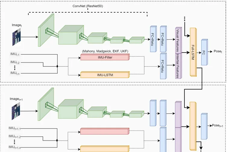
The main objective of this architecture is to estimate the global position accurately by minimizing the geometric con-sistencies loss function. This problem is formulated in the context of sequential, end-to-end, and multimodal training to estimate the global pose information. The global localization network exploits the outputs of CNN and LSTM in previous layers to have more and better knowledge of the environment. More specifically, the proposed neural network architecture is three-fold; a convNet network, a small IMU integrator bi-directional LSTM and global pose regressor bi-directional LSTM network for pose estimation. An overall view of the proposed architecture is shown in Figure 2.
Let’s suppose a sequential set of monocular RGB images (. . . , It−1, It, It+1, . . .) and IMU measurements
(. . . , IMUt−1, IMUt, IMUt+1, . . .) are given, the network
predicts the global pose pt = [xt, qt], where x ∈ R3
denotes the translation and q ∈ R4 denotes the rotation in quaternion representation. The input to the CNN and small LSTM streams are the image It and inertial measurement
IMUt, respectively, while the input to the global pose stream
is concatenation of features extracted by previous CNN and LSTM networks. The deep RCNN network effectively learns the following mapping, which converts image and IMU data input sequences to global poses:
DeepRCNN : {(RW ×H, R6)1:T} → {(R7)1:T} (1)
where W × H is the width and height of the input camera frames and 1 : T are the timesteps of the sequence. The rest of this section presents the constituent parts of this architecture and how the feature extractions and global localization are performed.
A. VISUAL-CNN FEATURE EXTRACTOR
A convNet is implemented to extract visual features from the monocular RGB image It and to make the process of
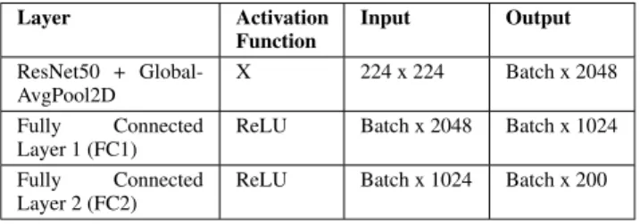
learning effective features suitable for the pose estimation automated. Instead of providing an aspect or visual context, the feature extraction is ideally geometrical, as there is a need for pose estimation frameworks to be generalized and applicable in environments not seen before. The Visual-CNN feature extractor configuration is listed in Table 1.
It is based on the architecture of ResNet-50 and also optical flow estimation network [83]. The ResNet50 is truncated prior to the last average pooling layer and the softmax layers are removed. A batch normalization and a rectified linear unit (ReLU) follow each convolution layer. The average pool-ing is then replaced by the global average poolpool-ing, which then adds two fully connected layers (FC). The output of the final convolutional layer is flattened and given as input to the first FC layer. Finally vector zI of the visual features is obtained
TABLE 1.Visual-CNN feature extractor configuration.
TABLE 2.IMU-LSTM feature extractor configuration.
by the second FC layer.
zI = VisualCNN(RW ×H) (2)
Instead of preprocessed images or point clouds, the CNN takes raw RGB images It as input, since the Visual-CNN
learns to extract optimal features for the pose estimation with lower dimensionality. In addition to lowering the high level of dimensionality in image of RGB in a compact vector, these learned feature representations improve the sequential training process. Therefore, for sequential modeling, the last convolutional features are passed to the Full-LSTM.
B. IMU-LSTM FEATURE EXTRACTOR
In the problem of visual inertial pose estimation, there is a challenge in processing the IMU measurements as they are received at a higher rate (e.g. 100 - 300 Hz) than camera frame rate (e.g. 10 - 30 Hz). To handle this in the proposed net-work, a small bi-directional LSTM inspired by [84] processes batches of raw inertial data IMUtbetween continuous camera
data forming 6 dimensional vector and its corresponding feature vector zIMU is given as output.
zIMU = IMULSTM(R6) (3)
Table 2 shows the configuration of the IMU-LSTM feature extractor module. The IMU-LSTM takes a batch of raw iner-tial measurements between two subsequent camera frames in the form of IMUt = (αt, ωt) ∈ R6, where αt ∈ R3is
linear acceleration andωt ∈ R3is angular velocity. The IMU
module receives the same size of padded input in each time frame. This processing module uses two sequential branches consisting of one bi-directional LSTM and one FC layer. The output feature vector of the FC layer is then carried over to the Full-LSTM.
C. FULL-LSTM POSE REGRESSOR
The configuration of the Full-LSTM pose regressor is presented in Table 3. The fundamental principle of pose estimation demands modeling temporal dependencies to
FIGURE 2. Architecture of the proposed Deep RCNN pose estimation system.
derive connections between sequential features. Hence, a bi-directional Full-LSTM takes as input the concatenated feature
zt = concat(zI, zIMU) together with its hidden previous
states ht−1. By leveraging hidden states present between
the sequences, LSTM utilizes the dynamics and temporal relationship of the sequential inputs. After the Full-LSTM, a fully connected layer serves as the pose estimator. It is of dimension 7 for the regression of translation and rotation in quaternion as x and q, respectively. Overall, the fully connected layer transforms the vector representation zt of
features into a pose vector as follows:
xt = FullLSTM(zt, zht−1) (4)
D. LOSS FUNCTION
As for pose estimation, the translation and orientation of the robot is estimated inspired by Wang et al. [85]. Here, the pose estimation is considered as a probabilistic problem. That is, the set of sequential poses Xt, their corresponding sequence
of camera images It and IMU data IMUt up to to time t are
given as follows:
Xt =(x1, x2, . . . , xt) (5)
TABLE 3.Full-LSTM global pose regressor configuration.
It =(i1, i2, . . . , it) (6)
IMUt =(imu1, imu2, . . . , imut) (7)
dt =(it, imut) (8)
Dt =(d1, d2, . . . , dt) (9)
Then
P(Xt | Dt) = P(x1, x2, . . . , xt | d1, d2, . . . , dt) (10)
It is possible to learn optimal weightsθ∗ by optimizing Equation 10.
θ∗
The L2 norm of ground truth xt = (ptT, ωtT)T and its
estimate ˆxt = (ˆptT, ˆωtT)T at time t based on MSE, can
therefore be reduced using θ∗ = argmin1 T T X t=1 k ˆpt− pt k22+λ k ˆωt−ωt k22 (12)
where p andω are translation and orientation along with k · kandλ representing the L2 distance and a scale factor to balance the weights of translations and orientations. Theω is represented in quaternions since the Euler representations might face issues in the global coordinate frame.
E. IMU-FILTER 1) MAHONY
The Mahony filter [86] is a Complementary filter which esti-mates the attitude, angle and orientation by fusing gyroscope measurements with accelerometer measurements. To do this, Mahony first computes orientation error from previous esti-mates using accelerometer measurements.
et+1 = It+aˆ 1× v(I q
t) (13)
ei,t+1 = ei,t+ et+11t (14)
where It+aˆ 1 denotes the normalized accelerometer measure-ments, v(Itq) is the orientation in quaternion and 1t is the timestamp between t and t + 1. Next is to fuse and estimate the orientation using incremental orientation between time t and t + 1. It+ω1= It+ω1+ Kpet+1+ Kiei,t+1 (15) 1IW t+1= 1 2I ˆ W t ⊗[0, It+ω1] T (16) It+W1= ItWˆ +1IW t+11t (17)
Here, It+ω1is updated gyro after fusion,1It+W1is orientation increment from gyro measurements and It+W1is the estimated orientation after integration of orientation increment.
2) MADGWICK
The Madgwick filter [87] also formulates the issue of ori-entation estimation in a quaternion space and the idea is to estimate It+W1fusing angular velocity and acceleration mea-surement by gyroscope and accelerometers. First step is the gradient step which computes orientation increment from accelerometer measurements. It+a1= −βargminf(I ˆ W t , Wgˆ, It+aˆ 1) k f(ItWˆ, Wgˆ, It+aˆ 1) k (18) where It+a1denotes the attitude component from accelerom-eter measurements, ItWˆ is orientation in quaternion, Wgˆ is
normalized gravity and It+aˆ 1is the normalized accelerometer measurements. Second step is to compute the orientation increment from gyro and finally fuse it with accelerometer measurements to obtain the estimated orientation.
1It+ω1 = 1 2I ˆ W t ⊗[0, It+ω1]T (19) 1IW t+1 =1It+ω1+ It+a1 (20) It+W1 = ItWˆ +1IW t+11t (21)
Here,1It+ω1is the gyro orientation increment,1It+W1is the fused orientation increment of gyro and accelerometer and
It+W1is the estimated orientation.
3) EKF
Real life system dynamics and observation models are rarely globally linear. However, they are often approximated well as linear functions locally. In order to linearize these functions the Taylor Expansion and Jacobians could be used and the EKF uses them to linearize the KF system. Here, the prior
p(x0) is a Gaussian distribution (i. e. p(x0) ∼ N (µ0, 60))
where x = [qwqx qyqzωx ωyωz] is a state vector of 7 states
to estimate the attitude. The continuous time process model ˆ
x = f(x, u, n) is non-linear with additive white Gaussian Noise Qt. The observation model h(x, v) is non-linear with
additive white Gaussian Noise Rt.
The linearization of dynamics model and observation model are done by
xt+1 ≈ f(xt, t) + Qt (22)
zt ≈ h(xt, t) + Rt (23)
After initializing the state vector ˆx0−and state covariance
P−0 matrices, the Kalman gain matrix is computed
Kt = P−t HtT[HtP−t HtT + Rt]−1 (24)
where Ht ≈ϑhϑx |x= ˆx−
t . Next is to calculate the state correction
vector and update state vector by ˆ xt = ˆxt−+ Kt[zt − ˆz−t ], with ˆz − t = h(ˆx − t , t) (25)
And the error covariance is update by
Pt =[I − KtHt]P−t (26)
The prediction of new state vector and state covariance vector matrices are done using
ˆ xt+−1= f(ˆxt, t) (27) P−t+1=8tPt8Tt + Qt (28) where8t =ϑfϑxt |x= ˆx− t . 4) UKF
The UKF used here is inspired by [88] that processes the estimated state and covariance matrix by the actual system dynamics. Just like EKF, nonlinear processes are managed by this method. The filter begins by initializing with a process noise Q, measurement noise R and a covariance P the same as the EKF. However, upon this step the disturbances are cal-culated from the covariance process noise using the Cholesky Decomposition. We have a state vector of 7 states to estimate the attitude.
The Kalman gain could be computed by:
K = PxzP−1vv (30)
where, Pxzand Pvvdenote cross correlation matrix and
inno-vation covariance. For the details on the calculation of these two variables referring to reference paper [88] is suggested.
With the Kalman gain computed, the state estimate and the state covariance can be updated as follows.
Pt+1 = ˆPt− KPvvKT (31)
ˆ
xt+1 = ˆxt+ K(ˆz − ¯Z) (32)
where, Pt+1denotes updated covariance, ˆPt is the estimated
covariance, ˆxt+1 is the updated state, ˆxt is the estimated
state, ˆz is the measurement readings and ¯Z is the estimated measurement readings.
IV. EXPERIMENTATION AND RESULTS
In this section, the performance of proposed Deep RCNN for global localization is evaluated and compared with the various popular and recent approaches developed for posi-tion estimaposi-tion of UAVs in terms of computaposi-tion time and position precision. Moreover, a comparison of IMU-LSTM and IMU-Filter based pose estimators are also presented by detailed analysis.
A. DATASET
EuRoC Dataset: EuRoC dataset [89] is frequently used in
evaluating VIO algorithms and is shared publicly by ETH. The dataset is collected by flying a UAV in two completely different envrionments and contains 11 sequences of Cam-era, IMU and LiDAR ground truth data. It comprises the synchronized stereo grayscale frames and IMU information with corresponding trajectory ground truth having frame rates of 20Hz, 200Hz and 100Hz respectively. Position ground truth values were measured with a Leica MS50 laser tracker and Vicon motion capture system. In addition, the database is categorized in three levels in terms of difficulty. These levels are easy, medium and difficult which are classified based on the image brightness level, image blurring, flight motion speed, etc. Such categorization of dataset lets the VIO algorithms deal with different challenges and therefore creation of better VIO methods. The Vicon Room dataset containing 6 sequences (V1_01-03, V2_01-03) at different levels of difficulty were used in this paper.
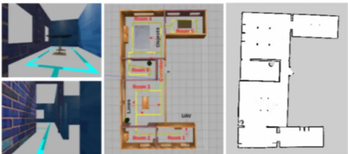
Simulation Dataset:For collecting simulation dataset, the Gazebo [90], an open-source library designed to simulate the real world, is used. It can be used as a plugin to Robotic Operating System (ROS) [91] and simulate environments compatible to it. We collect training data in the virtual environment retrieved from the ROS. Figure 3 shows the simulation environment and its 2D grid map obtained by Hokuyo UTM-30LX installed on a Turtlebot 3 Waffle Pi along with sample camera views of Tello UAV. The UAV collects all the information in the simulation environment, which randomly flies and lands at constant speed indoors.
FIGURE 3. Simulation environment, its 2D grid map and sample camera views of Tello UAV.
It collects the timestamped ground truth position of UAV in dimension of R3and orientation in dimension of R4at the rate of 300Hz. The IMU and camera sensors data were collected at the rate of 300Hz and 30Hz, respectively. The preprocessing and synchronization of ground-truth and sensors data were then performed. With the required pose measurements from the data collected in simulation, the RGB camera frames were labeled accordingly. Lastly, in order to minimize processing costs, the image resolutions were reduced to 640 x 480.
Real-World Experiment: In order to better evaluate the
performance of the proposed Deep RCNN architecture on the global pose estimation, a real-world experiment was per-formed using the DJI Tello drone in an indoor laboratory environment. The training dataset was collected from a 20 x 15-meter sized laboratory containing different objects (e. g., chairs, tables, computers, ground and aerial robots, etc.), making the environment textured. All implementations were done on the ROS framework using the python programming language. Since the Tello is a low-cost drone with minimal processing power, it was only used to collect monocular images, IMU measurements, and ground truth poses. The main pose estimation process was performed on a remote processing unit connected to the Tello drone via the wireless connection. The drone sends real-time information to the remote processing unit through topics published by ROS packages and receives the control commands the same way vice versa.
During the data collection, it was observed that the real drone experiment differs from simulation and other datasets in at least two ways. An issue faced during the experiment was the asynchronous data collection. The fact that the visual data received from the Tello drone was in h264 compressed video format made the data synchronization difficult. In order to handle this issue, a real-time encoder was implemented fol-lowed by an interpolation technique to synchronize the visual, IMU, and ground truth information into a 30Hz frame rate. The second difference from the simulation environment was the quality of the Tello drone’s visual information. Since the data are encoded from h264 compressed videos and collected through a wireless connection, the visual data faced quality degradation, as shown in Figure 4. However, as demonstrated in section 4.4.3, the proposed Deep RCNN architecture was capable of handling the degraded visual data without a severe negative effect on the global pose estimation performance.
FIGURE 4. DJI Tello drone and its sample degraded images collected from laboratory.
B. NETWORK TRAINING
All the demonstrated experiments were carried out on an Intel(R) Core(TM) i7-9750H CPU @ 2.60GHz processor system loaded with 16 GB DDR3 RAM and NVIDIA GeForce GTX 1660Ti GPU. To evaluate the pose estima-tion learning process and GPU implementaestima-tions, the Ten-sorflow framework [92], developed by Google Brain team. The entire data preprocessing was implemented in Python, using relevant libraries compatible with the python bindings of Tensorflow.
In order to obtain best features from monocular images, the transfer learning technique is used in CNN feature extractor module of proposed deep pose estimator. Here, the ResNet50 model is used with the last classification layer removed as explained in section 3.1. Since the ResNet50 accepts input images of size 224×224×3, the images have been downsized accordingly. The full network is trained for 100 epochs using a batch size of 64 which took on average 3 hours per dataset. The ADAM [93] is used as the optimization function with learning rate = 1e − 4, decay = le−2004 and error function of mean absolute error (MAE).
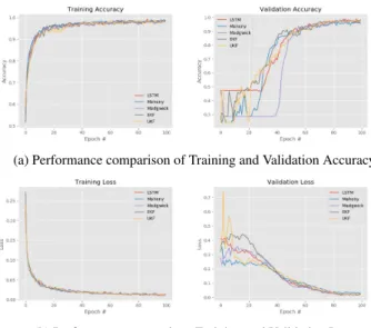
Figure 5 demonstrates the training and validation loss and accuracy for EuRoC sequence V1_02_medium using five different setups of Deep RCNN: red curve depicts the training accuracy and loss of Deep RCNN localization with IMU-LSTM only, blue curve is the accuracy and loss trained with Mahony, purple is the accuracy and loss trained with Madgwick, gray and yellow curves are the accuracy and loss of VIO trained with EKF and UKF respectively. It can be observed that the convergence of the network on the training set is the same for all network forms. However, in the vali-dation set the convergence of accuracy is faster for EKF and UKF compared to other forms of network. For the validation loss graph the UKF and Mahony have the faster convergence. It is worth noting that the LSTM form of the network has the
FIGURE 5. Comparison of training and validation accuracy (top) and loss (bottom) using five forms of network on sequence V1_02_medium of EuRoC dataset.
medium performance on both validation accuracy and loss graphs.
C. EVALUATION METRIC
In order to assess the performance of proposed global local-ization framework, the root mean square error (RMSE) of the translation and rotations are calculated and compared with the popular standard and deep methods in [94]–[105]. In other terms, errors in position and orientation along the whole trajectory were calculated and compared with ground truth. For regression problems, the RMSE calculated the standard deviation of the difference between predicted and ground truth values RMSE = s PI i=1(ˆxi− xi)2 n (33)
where x is the ground truth and ˆx is the predicted value. Moreover, to quantitatively evaluate the effects of filter based methods compared to IMU-LSTM on the performance of pose estimation, the time taken to process each frame in end-to-end pose estimation is considered as the metric.
D. COMPARISON OF IMU-LSTM AND IMU-FILTER
In order to quantify the performance of Deep RCNN based position estimators, we first compare the IMU-LSTM based setup with filter based (Mahony, Madgwick, EKF, UKF) ones. We compare these setups in terms of position estimation accuracy and time-efficiency on both simulation and public EuRoC datasets.
1) SIMULATION
In the simulation environment, the 3D ground truth motion carried by Tello is shown in Figure 6. It consists of a total of 2432 camera frames and 24320 IMU measurements.
FIGURE 6. Ground Truth Trajectory for the tested simulation environment.
FIGURE 7. Comparison result of IMU-LSTM based and IMU-Filter based position estimation setup on simulation environment.
As seen in this figure, the trajectory during the orientation change is very sharp-edged which makes the learning state estimation procedure somehow difficult for the network.
In Figure 7, the comparison result of Deep RCNN based position estimation framework with different network setups on the simulation dataset is given. Here, it is observed that the IMU-LSTM setup has the better performance in terms of accuracy compared to filter based alternatives. However, it does not perform as fast as filter based methods. In terms of time-efficiency, the filter based methods have better per-formance and specifically the EKF setup has the best perfor-mance followed by UKF.
2) EuRoC
In this section, the results of IMU-LSTM setup of Deep RCNN based position estimation framework is presented in comparison to the filter-based Deep RCNN position estimators. The experiments are performed on the EuRoC dataset using three challenging categories of sequences (easy, medium, difficult). In the training process, the dataset was split into two sets of testing and training. The train and test datasets contained 75% and 25% of each sequence respec-tively. For the ease of model understanding, we first tested each of our transfer learning and LSTM models separately
FIGURE 8. The IMU-LSTM sub-model’s results on the sequence V1_01 of EuRoC dataset.
on images and IMU data on the datasets. The ResNet50 was able to extract sufficient features from the images. The LSTM model also was able to predict the next IMU measurements in a normalized manner which made the training process and the pose prediction more stable.
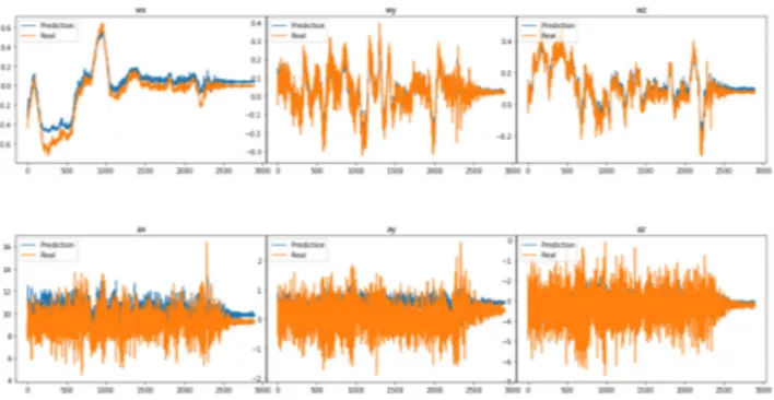
Figure 8 shows the IMU-LSTM sub-model’s results on the sequence V1_01 of EuRoC dataset. Here, the gyroscope and accelerometer measurements are each represented in 3 axises by (wx, wy, wz) and (ax, ay, az), respectively. The orange curve depicts the biased IMU measurements and the blue curve represents the filtered IMU measurements obtained by the IMU-LSTM sub-model. The results indicate that the IMU-LSTM sub-model provides normalized IMU data values by considering the temporal dependencies between IMU measurements. This normalization process helps to handle the IMU noises available in the measurements. The best-estimated values are observed in the gyroscope measure-ments, where the predicted values are better normalized and estimated. In the accelerometer measurements, the impact is less compared to the gyroscope due to the accelerometer0s
high vibration noise. These normalized values are then used as IMU input to the IMU-LSTM setup of Deep RCNN net-work to estimate the global pose of the robot.
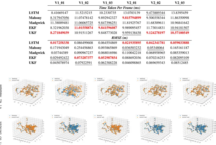
In Figure 9, the qualitative comparison of 3D trajectories obtained from IMU-LSTM, IMU-Mahony, IMU-Madgwick, IMU-EKF and IMU-UKF setup of Deep RCNN based pose estimation architecture on the EuRoC dataset’s V1_02 sequence. All the 5 setups can deliver fairly good results on both sequences despite their difficulty levels where V1_03_difficult contained frames with more illumination inconsistencies and motion speed causing blurry images.
3) REAL-WORLD EXPERIMENT
This experiment was conducted on the known laboratory environment mentioned in section 4.1, with data segregated into training and testing sequences in 75% and 25% ratios, similar to the other experiments mentioned above. As shown in Table 5, the performance comparison was performed among five different setups of Deep RCNN for global local-ization in terms of time efficiency and RMSE. The results demonstrate that similar to simulation and EuRoC experi-ments, the IMU-LSTM setup of the network performs better
TABLE 4. Comparison result of IMU-LSTM based and IMU-Filter based position estimation setups on EuRoC dataset. The upper part shows the comparison of 5 setups of deep RCNN based global pose estimators in terms of time taken in milliseconds to process each frame and its corresponding IMU measurements. The results demonstrate that the IMU-Filter setups outperform IMU-LSTM one on all sequences. The time difference among IMU-Filter setups are minor compared to IMU-LSTM setup. The lower part of the table shows their pose estimation accuracy comparison in terms of RMSE and the results show that the IMU-LSTM setup has better performance compared to IMU-Filter on all sequences except V1_02 and V1_03. In these two sequences the IMU-EKF and IMU-UKF alternative setups have achieved better accuracy compared to IMU-LSTM setup.
FIGURE 9. Trajectory Comparison of IMU-LSTM based and IMU-Filter based position estimation setups on EuRoC sequences V1_02 (top) and V1_03 (bottom) (Left to Right: LSTM, Mahony, Madgwick, EKF, UKF).
TABLE 5. Comparison result of IMU-LSTM based and IMU-Filter based position estimation setups on real-time experiment.
in terms of accuracy, with the cost of being slower in process-ing frames compared to its filter-based alternatives.
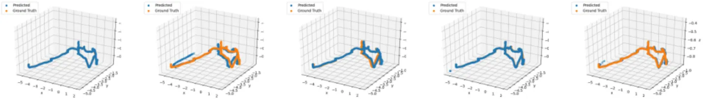
To analyze the localization performance qualitatively concerning the tested environment, we present a trajectory visualization that shows the pose estimate obtained from five different setups of the Deep RCNN framework compared to the ground truth. Figure 10 displays the results of this exper-iment. The predicted poses are shown as a blue trajectory, and the ground truth poses are shown as an orange trajectory.
This displays that all five setups’ performances are compara-ble to each other with minor accuracy difference even with the presence of degraded monocular images, as shown in Figure 4. The IMU-LSTM setup demonstrated the minimum error rate, and the IMU-Mahony has the highest error rate compared to other setups.
E. COMPARISON TO LITERATURE
In order to show an empirical comparison to the closest related methods in the literature, we compare our approach to a selection of state-of-the-art traditional and learning based VO, VIO, and V-SLAM methods [94]–[105]. The tradi-tional methods include SVOMSF [95], MSCKF [96], OKVIS [97], ROVIO [98], VINSMONO [99], VINSMONO+LC [100], SVOGTSAM [101], ORBSLAM2 [12], STCM-SLAM [102] and learning based are SelfVIO [103], Kimera [104] and methods proposed by Baldini et al. [94] and Li and Steven [105]. The dataset used for this evaluation is EuRoC’s V1_01-03, V2_01-03 sequences.
FIGURE 10. Trajectory Comparison of IMU-LSTM based and IMU-Filter based position estimation setups on real-world experiment (Left to Right: LSTM, Mahony, Madgwick, EKF, UKF).
TABLE 6. Comparative results for EuRoC (V1_01-03, V2_01-03) sequences.
Table 6 shows the comparative results for these sequences. It is observed that the proposed architecture consistently out-performs existing methods for all sequences in terms of pose estimation accuracy. In particular, the highest improvement was obtained in the more difficult and challenging sequences that contain textureless and blurred camera frames. As illus-trated, traditional methods handle high quality and feature-ful images, but fail with feature-full sensor degradation and image occlusions due to their geometrical algorithm limitations and not benefiting from temporal information. From the observed results, the inference is that conventional visual-based pose estimation methods are not an appropriate approach for local-ization in the presence of occluded or textureless visual data and when the IMU measurements are not tightly synchro-nized. In addition, the estimation accuracy of the proposed architecture is superior to the learning based methods listed in Table 6. It is worth noting that, proposed method is able to take the temporal constraints into account that helps it to generalize for unseen scenarios to some extent.
F. ABLATION STUDY
In order to demonstrate the effectiveness of each module and the overall architecture of Deep RCNN, we evaluate various setups of our method on the EuRoC dataset, simulation envi-ronment, and real-world experiment in the ablation section. Figures 7-10 and tables 4-6 display the best performance results in bold and the second-best in underlined.
First, we evaluate our method on pose estimation of a drone in a simulation environment (section 4.4.1). It includes training the Deep RCNN network using five different setups
on the dataset collected from the simulation environment and testing the trained model to pose estimation of a drone in the same simulation environment. It can be seen from Figure 7, even though the simulation environment has many similar or no wall textures (where traditional geometric methods struggle to deal with feature extraction and matching), our network setups still show considerably high accuracy with fairly low processing cost. The results also indicate that the IMU-LSTM setup can benefit from temporal features of IMU and therefore reduce RMSE error compared to its filter-based alternatives. On the other hand, the filter-based methods reduce the time taken to process each frame with the cost of increasing the RMSE compared to their LSTM alternative.
Second, we compare our Deep RCNN architecture’s efficiency on a common indoor benchmark dataset called EuRoC. Since this dataset contains three different difficulty levels, our focus was to test our architecture in dealing with more challenging visual data like blurred images and high-speed velocity changes. The results are depicted in Table 4 and Figure 9. It can be seen that, although the dataset contained very blurred images and in situations where the visual data brightness are overexposed or very low, the Deep RCNN network is able to reduce RMSE error to some extent, indicating that it is capable of dealing with high motion speeds in various illuminations. In comparing five network setups, the general outcome of the simulation environment holds here too, where the IMU-LSTM utilizes the temporal dependency in IMU data and thus has better RMSE compared to filter-based setups. However, the filter-based methods per-form better in the case of time-efficiency.
Finally, to study the effect of Deep RCNN architecture on the real-time global localization of a UAV, a real-world experiment was performed using a DJI Tello drone in an indoor laboratory environment. In this experiment, it was observed that the data received from the drone depends on the UAV components’ quality and the connection between the UAV and the remote processing unit. For instance, in the experiment, the DJI Tello drone’s data was highly desynchro-nized, and the visual data was degraded (Figure 4). However, as demonstrated in Table 5 and Figure 10, the results show that this visual degradation does not negatively impact the accuracy and the Deep RCNN architecture is capable of han-dling it. In addition, compared with filter-based setups, the IMU-LSTM version provides a further boost to the pose esti-mation accuracy. As mentioned in the previous paragraph, the reason is that IMU-LSTM integrates temporal correlations and previous experience over window sequences between IMU measurements. Besides, filter-based setups tend to form better than IMU-LSTM in time-efficiency. The per-formance difference among filter-based setups themselves changed for various tests and was negligible.
V. DISCUSSION AND FUTURE WORK
The proposed method demonstrates competitive performance on the EuRoC dataset and simulation environment. From the results, it can be observed that the proposed method works significantly better than its camera-only or IMU-only traditional and learning based alternative methods. Fusing visual information with inertial measurements positively affects the performance of the DL based pose estimation by adding historic knowledge lying in IMU data hence signif-icantly improving position estimations. This indicates that these kinds of DL based VIO architectures can be tested on real-time robotic platforms.
Observing the results, it is apparent that the more the network knows about a specific scene, the better it gets to estimate position. However, this could lead to the problem of overfitting and the trained model lacking the generalization capability. Moreover, the additional downside of supervised DL methods is the need for ground truth labels and the fact that data need to be trained for all scenarios of challenges (e.g. different weather and environment dynamicity). In case the training data does not hold the latter condition, the resulting trained model will lack the generalization characteristic and will not be usable in real world applications.
Some approaches in order to tackle these issues and develop a robust and powerful DL based pose estimation or SLAM systems could be:
• More sensor data and better fusion algorithms: Beyond
the camera and IMU sensors, the use of information from other sensors such as LiDAR, thermal camera, mmwave device and Radar may let the DL based localization systems to have more accurate and robust estimations particularly in harsh weather or low-light situations. Moreover, the fusion of these sensor data is
a way to research. Not many DL-based pose estimation studies have focused on sensor fusion algorithms in DL-based systems. Therefore, the use of multimodal sensors and enhanced fusion algorithms has the potential to produce more robust systems.
• Unsupervised/Adaptive Learning: Using
unsuper-vised/adaptive learning methods could boost the perfor-mance of DL based methods by eliminating the need for large amounts of training data. Such methods allow DL methods to generalize and adapt to unseen and dynamic environments by predicting poses or scenes.
• Semantic information: The semantic information present in the camera images could enhance DL based approaches by incorporating more understanding of the environment and more semantic reasoning. This knowl-edge led the device to detect the objects surrounding the robot and to make localization decisions based on that information. Such information can also help the robot navigate by providing more information to the control commands.
• Hybrid systems: combining the advantages of DL based
methods and traditional methods may lead to a hybrid system. The robust feature detection ability of DL com-bined with loop closing and efficient optimization capa-bilities of traditional methods could improve the pose estimation and SLAM systems.
VI. CONCLUSION
In this study, a sequential, end-to-end, and multimodal DL based monocular visual-inertial localization system is pro-posed to resolve the problem of global pose regression for UAV in indoor scenarios. In addition a filter based IMU alter-native to IMU-LSTM is provided to enhance the computa-tion efficiency without degrading the accuracy. The proposed deep global positioning is compared in terms of accuracy with various state-of-the-art algorithms for public EuRoC dataset and simulation environments. Furthermore, a thorough com-parison of Filter based and LSTM based deep RCNN has been carried out in terms of accuracy and time-efficiency. Experi-mental findings demonstrate a high degree of time efficiency and promising accuracy in UAVs indoor localization with the proposed filter based deep RCNN.
ACKNOWLEDGMENT
The authors also would like to thank the Konya Technical University RAC-LAB Research Laboratory (www.rac-lab.com).
REFERENCES
[1] S. Thrun, W. Burgard, and D. Fox, Probabilistic Robotics. Cambridge, MA, USA: MIT Press, 2005.
[2] B. Siciliano and O. Khatib, Springer Handbook of Robotics. Cham, Switzerland: Springer, 2016.
[3] C. Chen, B. Wang, C. Xiaoxuan Lu, N. Trigoni, and A. Markham, ‘‘A survey on deep learning for localization and mapping: Towards the age of spatial machine intelligence,’’ 2020, arXiv:2006.12567. [Online]. Available: http://arxiv.org/abs/2006.12567
[4] F. Fraundorfer and D. Scaramuzza, ‘‘Visual odometry: Part ii: Matching, robustness, optimization, and applications,’’ IEEE Robot. Automat. Mag., vol. 19, no. 2, pp. 78–90, Feb. 2012.
[5] D. Nistâer, O. Naroditsky, and J. Bergen, ‘‘Visual odometry,’’ in Proc. IEEE Conf. Comput. Vis. Pattern Recognit., Jun. 2004, pp. 652–659. [6] D. Scaramuzza and F. Fraundorfer, ‘‘Visual Odometry [Tutorial],’’ IEEE
Robot. Autom. Mag., vol. 18, no. 4, pp. 80–92, Dec. 2011.
[7] A. I. Comport, E. Malis, and P. Rives, ‘‘Real-time quadrifocal visual odometry,’’ Int. J. Robot. Res., vol. 29, nos. 2–3, pp. 245–266, Feb. 2010. [8] N. Krombach, D. Droeschel, and S. Behnke, ‘‘Combining feature-based and direct methods for semi-dense real-time stereo visual odometry,’’ in Proc. Int. Conf. Intell. Auton. Syst., 2016, pp. 855–868.
[9] J. Engel, V. Koltun, and D. Cremers, ‘‘Direct sparse odometry,’’ IEEE Trans. Pattern Anal. Mach. Intell., vol. 40, no. 3, pp. 611–625, Mar. 2018. [10] C. Forster, M. Pizzoli, and D. Scaramuzza, ‘‘SVO: Fast semi-direct monocular visual odometry,’’ in Proc. IEEE Int. Conf. Robot. Autom. (ICRA), May 2014, pp. 15–22.
[11] R. Mur-Artal, J. M. M. Montiel, and J. D. Tardos, ‘‘ORB-SLAM: A versatile and accurate monocular SLAM system,’’ IEEE Trans. Robot., vol. 31, no. 5, pp. 1147–1163, Oct. 2015.
[12] R. Mur-Artal and J. D. Tardos, ‘‘ORB-SLAM2: An open-source SLAM system for monocular, stereo, and RGB-D cameras,’’ IEEE Trans. Robot., vol. 33, no. 5, pp. 1255–1262, Oct. 2017.
[13] A. Vakhitov, V. Lempitsky, and Y. Zheng, ‘‘Stereo relative pose from line and point feature triplets,’’ in Proc. Eur. Conf. Comput. Vis. (ECCV), 2018, pp. 648–663.
[14] J. Engel, T. Schöps, and D. Cremers, ‘‘LSD-SLAM: Large-scale direct monocular SLAM,’’ in Proc. Eur. Conf. Comput. Vis. Cham, Switzerland: Springer, 2014.
[15] J. Engel, J. Sturm, and D. Cremers, ‘‘Semi-dense visual odometry for a monocular camera,’’ in Proc. IEEE Int. Conf. Comput. Vis., Dec. 2013, pp. 1449–1456.
[16] N. Yang, R. Wang, X. Gao, and D. Cremers, ‘‘Challenges in monoc-ular visual odometry: Photometric calibration, motion bias, and rolling shutter effect,’’ IEEE Robot. Autom. Lett., vol. 3, no. 4, pp. 2878–2885, Oct. 2018.
[17] D. Schubert, N. Demmel, V. Usenko, J. Stuckler, and D. Cremers, ‘‘Direct sparse odometry with rolling shutter,’’ in Proc. ECCV, 2018, pp. 682–697. [18] B. Zhuang, Q.-H. Tran, P. Ji, L.-F. Cheong, and M. Chandraker, ‘‘Learn-ing structure-and-motion-aware roll‘‘Learn-ing shutter correction,’’ in Proc. IEEE/CVF Conf. Comput. Vis. Pattern Recognit. (CVPR), Jun. 2019, pp. 4551–4560.
[19] O. Bogdan, V. Eckstein, F. Rameau, and J.-C. Bazin, ‘‘DeepCalib: A deep learning approach for automatic intrinsic calibration of wide field-of-view cameras,’’ in Proc. 15th ACM SIGGRAPH Eur. Conf. Vis. Media Prod., 2018, pp. 1–10.
[20] B. Zhuang, Q.-H. Tran, G. H. Lee, L. F. Cheong, and M. Chandraker, ‘‘Degeneracy in self-calibration revisited and a deep learning solution for uncalibrated SLAM,’’ in Proc. IEEE/RSJ Int. Conf. Intell. Robot. Syst. (IROS), Nov. 2019, pp. 1–8.
[21] S. Ren, K. He, R. Girshick, and J. Sun, ‘‘Faster R-CNN: Towards real-time object detection with region proposal networks,’’ in Proc. Adv. Neural Inf. Process. Syst., 2015, pp. 91–99.
[22] A. Krizhevsky, I. Sutskever, and G. E. Hinton, ‘‘Imagenet classification with deep convolutional neural networks,’’ in Proc. Adv. Neural Inf. Process. Syst., 2012, pp. 1097–1105.
[23] J. Long, E. Shelhamer, and T. Darrell, ‘‘Fully convolutional networks for semantic segmentation,’’ in Proc. IEEE Conf. Comput. Vis. Pattern Recognit. (CVPR), Jun. 2015, pp. 3431–3440.
[24] R. Clark, S. Wang, H. Wen, A. Markham, and S. Wang, ‘‘Vinet: Visual inertial odometry as a sequence-to-sequence learning problem,’’ in Proc. 31st AAAI Conf. Intell., May 2017, pp. 3995–4001.
[25] A. Kendall, M. Grimes, and R. Cipolla, ‘‘PoseNet: A convolutional network for real-time 6-DOF camera relocalization,’’ in Proc. IEEE Int. Conf. Comput. Vis. (ICCV), Dec. 2015, pp. 2938–2946.
[26] R. Clark, S. Wang, A. Markham, N. Trigoni, and H. Wen, ‘‘VidLoc: A deep spatio-temporal model for 6-DoF video-clip relocalization,’’ in Proc. IEEE Conf. Comput. Vis. Pattern Recognit. (CVPR), Jul. 2017, pp. 6856–6864.
[27] H. Bay, T. Tuytelaars, and L. Van Gool, ‘‘Surf: Speeded up robust fea-tures,’’ in Proc. Eur. Conf. Comput. Vis. Berlin, Germany: Springer, 2006, pp. 407–417.
[28] M. Trajkoviá and M. Hedley, ‘‘Fast corner detection,’’ Image Vis. Com-put., vol. 16, no. 2, pp. 75–87, Feb. 1998.
[29] D. G. Lowe, ‘‘Distinctive image features from scale-invariant keypoints,’’ Int. J. Comput. Vis., vol. 60, no. 2, pp. 91–110, Nov. 2004.
[30] E. Rublee, V. Rabaud, K. Konolige, and G. Bradski, ‘‘ORB: An efficient alternative to SIFT or SURF,’’ in Proc. Int. Conf. Comput. Vis., Nov. 2011, pp. 2564–2571.
[31] C. Harris and M. Stephens, ‘‘A combined corner and edge detector,’’ in Proc. Alvey Vis. Conf., 1988, p. 50.
[32] C. Tomasi and T. Kanade, ‘‘Shape and motion from image streams: A factorization method-3. Detection and tracking of point features,’’ Carnegie Mellon Univ., Pittsburgh, PA, USA, Tech. Rep. CMU-CS-91-132, 1991.
[33] J. Shi and C. Tomasi, ‘‘Good features to track,’’ in Proc. IEEE Comput. Soc. Conf., Jun. 1994, pp. 593–600.
[34] D. Nister, ‘‘An efficient solution to the five-point relative pose problem,’’ IEEE Trans. Pattern Anal. Mach. Intell., vol. 26, no. 6, pp. 756–770, Jun. 2004.
[35] P. Chang and M. Hebert, ‘‘Omni-directional structure from motion,’’ in Proc. IEEE Workshop Omnidirectional Vis., Jun. 2000, pp. 127–133. [36] D. Scaramuzza, A. Martinelli, and R. Siegwart, ‘‘A toolbox for easily
calibrating omnidirectional cameras,’’ in Proc. IEEE/RSJ Int. Conf. Intell. Robot. Syst., Oct. 2006, pp. 5695–5701.
[37] C. Engels, H. Stewãnius, D. Nistãr, B. Triggs, P. F. McLauchlan, R. I. Hartley, A. W. Fitzgibbon, M. Quigley, K. Conley, B. P. Gerkey, J. Faust, T. Foote, J. Leibs, R. Wheeler, and A. Y. Ng, ‘‘Bundle adjustment—A modern synthesis,’’ in Proc. ICRA Workshop Open Source Softw., vol. 2. Berlin, Germany: Springer, 2009, pp. 298–372.
[38] D. Scaramuzza, ‘‘1-Point-RANSAC structure from motion for vehicle-mounted cameras by exploiting non-holonomic constraints,’’ Int. J. Com-put. Vis., vol. 95, no. 1, pp. 74–85, Apr. 2011.
[39] B. Kitt, A. Geiger, and H. Lategahn, ‘‘Visual odometry based on stereo image sequences with RANSAC-based outlier rejection scheme,’’ in Proc. IEEE Intell. Vehicles Symp., Jun. 2010, pp. 486–492.
[40] L. Kneip, M. Chli, and R. Siegwart, ‘‘Robust real-time visual odometry with a single camera and an IMU,’’ in Proc. Brit. Mach. Vis. Conf., 2011, pp. 1–12.
[41] T. Kazik, L. Kneip, J. Nikolic, M. Pollefeys, and R. Siegwart, ‘‘Real-time 6D stereo visual odometry with non-overlapping fields of view,’’ in Proc. IEEE Conf. Comput. Vis. Pattern Recognit., Jun. 2012, pp. 1529–1536. [42] H. Jin, P. Favaro, and S. Soatto, ‘‘A semi-direct approach to structure from
motion,’’ Vis. Comput., vol. 19, no. 6, pp. 377–394, Oct. 2003. [43] N. Molton, A. Davison, and I. Reid, ‘‘Locally planar patch features for
real-time structure from motion,’’ in Proc. Brit. Mach. Vis. Conf., 2004, pp. 1–10.
[44] G. Silveira, E. Malis, and P. Rives, ‘‘An efficient direct approach to visual SLAM,’’ IEEE Trans. Robot., vol. 24, no. 5, pp. 969–979, Oct. 2008. [45] A. Pretto, E. Menegatti, and E. Pagello, ‘‘Omnidirectional dense
large-scale mapping and navigation based on meaningful triangulation,’’ in Proc. IEEE Int. Conf. Robot. Autom., May 2011, pp. 3289–3296. [46] R. A. Newcombe, S. J. Lovegrove, and A. J. Davison, ‘‘DTAM: Dense
tracking and mapping in real-time,’’ in Proc. Int. Conf. Comput. Vis., Nov. 2011, pp. 2320–2327.
[47] D. Scaramuzza, F. Fraundorfer, M. Pollefeys, and R. Siegwart, ‘‘Closing the loop in appearance-guided structure-from-motion for omnidirectional cameras,’’ in Proc. 8th Workshop Omnidirectional Vis., Camera Networks Non-Classical Cameras (OMNIVIS), Marseille, France, R. Swaminathan, V. Caglioti, and A. Argyros, Eds., Oct. 2008, pp. 1–15.
[48] H. Silva, A. Bernardino, and E. Silva, ‘‘Probabilistic egomotion for stereo visual odometry,’’ J. Intell. Robot. Syst., vol. 77, no. 2, pp. 265–280, Apr. 2014.
[49] H. Silva, A. Bernardino, and E. Silva, ‘‘A voting method for stereo egomotion estimation,’’ Int. J. Adv. Robot. Syst., vol. 14, no. 3, Jun. 2017, Art. no. 172988141771079.
[50] K. Konda and R. Memisevic, ‘‘Learning visual odometry with a convolu-tional network,’’ in Proc. 10th Int. Conf. Comput. Vis. Theory Appl., 2015, pp. 486–490.
[51] A. Nicolai, R. Skeele, C. Eriksen, and G. A. Hollinger, ‘‘Deep learning for laser based odometry estimation,’’ in Proc. Limits Potentials Deep Learn. Robot., 2016, pp. 1–5.
[52] G. Costante, M. Mancini, P. Valigi, and T. A. Ciarfuglia, ‘‘Exploring representation learning with CNNs for frame-to-frame ego-motion esti-mation,’’ IEEE Robot. Autom. Lett., vol. 1, no. 1, pp. 18–25, Jan. 2016.