ESKİŞEHİR TECHNICAL UNIVERSITY JOURNAL OF SCIENCE AND TECHNOLOGY A- APPLIED SCIENCES AND ENGINEERING
2018, 19(4), pp. 907 - 925, DOI: 10.18038/aubtda.413890
COMPARISON OF PROVINCES OF TURKEY IN TERMS OF ACCESSING HEALTH CARE SERVICES BY USING DIFFERENT CLUSTERING ALGORITHMS
Hasan YILDIRIM1*
1 Statistics, Kamil Özdağ Faculty of Science, Karamanoğlu Mehmetbey University, Karaman, Turkey
ABSTRACT
The most primary of the basic human rights is to have access to health care services. It is vital that all citizens in a country are able to get these services equally and homogeneously. Despite its importance, providing health services vary both internationally and nationwide in a country. Similarly, it may cause severe disparities and negative effects between individuals in a society. The primary concern of this study is to determine whether there is any difference between Turkey provinces in terms of accessing health care services, or not. Several clustering algorithms including hierarchical clustering, k-means and partitioning around medoids (pam) are applied to the data set including 31 health indicators for the provinces in Turkey. After comparing these algorithms via using some measures for determining the number of clusters and cluster validity, the findings show that there are four distinct and significant clusters based on k-means clustering algorithm. It seems that these clustering results are in a a close reciprocal relationship with the economic development and geographical location of provinces. Clustering results are evaluated and interpreted according to these two important findings.
Keywords: Cluster analysis, Health services, Hierarchical clustering, k means, Cluster validity
1. INTRODUCTION
Having access to health care services is the most primary of the basic human rights. It is vital that all citizens in a country are able to get these services equally and homogeneously. This is the necessity of health right defined as “accessing the highest health care standards which is possible” [1]. The definition of health right was firstly appeared in a universal document belongs to World Health Organization, in 1947 and given as “a birthright that is independently of race, religion, language, political view, economic and social conditions” [2].
Despite its importance, providing health services vary from both country to country and between different provinces or states in country. The standards of these services are well-balanced neither worldwide nor in a country itself. Consequently, this situation may cause severe disparities and negative effects between individuals in the society. In other words, there are likely to see preventable disparities in terms of getting the potential of being healthy between ones are part of different regions, communities and classes. Similar disparities can be found about sharing sources relevant to health services. Disparities in health care services is the major focus in Turkey health sector [2, 3].
In Turkey, some positive advances have been done in health sector by the program of transformation in health which has started in 2003. Physical and technical capabilities, labor force, financial conditions and infrastructure of health system have been reconstructed and enhanced. It seems that the positive effect of this situation increases from the east to the west of Turkey. Sharing of all health sources is in favor of the western provinces. So, the health indicators belong to east provinces are lower than the west [4,5]. In addition, there is a close reciprocal causality relationship between the health level of a society and economic development. The societies which have a certain level of economic development allocate higher share to the health. Thereby, the health awareness of individuals increases. Also, the development of health awareness expedites the economic develoment [5, 6].
The primary concern of this study is to look for some insights about the following questions: “Is there any imbalance between Turkey provinces in terms of accessing health care servies?” and “Is there any relationship between the location, development of a province and the level of health services?”. For this purpose, some health indicators for each province are provided from a research report of the ministry of health in Turkey [7]. Cluster analysis which is one of the most common used multivariate statistics techniques is used to examine these indicators. Different clustering algorithms results have been given comparatively. In the Section 2, literature review about related works has been summarised. The details of clustering algorithms used in this study have been mentioned in the Section 3. Some information about research problem, source of the data set and details of application process have been given in the Section 4. In the Section 5, the results of study have been presented. Lastly, conclusions has given in the Section 6.
2. RELATED WORKS
There are relatively few studies which are directly about heatlh care services. A great deal of previous researches into this topic have focused on human development index. Health indicators have been studied as a part of human development index. In other words, a health index representing health care services has been examined as a sub-measure of human development index and assessed a part of whole rather than individually in these kind of studies. This index consists of various socio-economic variables including some health indicators.
Hamarat [8] grouped the provinces of Turkey using health, population, economic and culturel indicators by applying cluster analysis. On the basis of squared euclid distance in Ward linkage, 8 clusters were found meaningful and significant. Besides, discriminant analysis was employed to determine whether each province was assigned to true cluster or not. Consequently both results were found agreeable. Çilan and Demirhan [9] performed hierarchical and non-hierarchical clustering methods and multidimensional scaling to find and visualize some meaningful clusters in Turkish provinces. The data set using in this study consisted of 27 socio-economic variables. As a result, average linkage was chosen and 7 clusters were formed.
Albayrak et al. [10] used principal component analysis which is one of the factor analysis methods to examine the development levels of Turkey provinces based on regions and gave the results comparatively.
Karabulut et al. [11] carried out a hierarchical cluster analysis based on 54 socio-economic variables on Turkish provinces. In this study, squared euclid and pearson proximity measures were used to calculate distances. The single linkage clustering method was employed to create clusters between provinces. By selecting the number of clusters intuitively, 7, 8 and 15 clusters were tested and interpreted. As a result, 15 meaningful clusters found in Turkish provinces.
Kaygısız et al. [12] found 5 clusters which is based on their data set in Turkish provinces by using Path and Cluster Analysis.
Filiz [13] applied various methods including discriminant analysis, principal components analysis, cluster analysis and multidimensional scaling analysis on a data set consisting of 16 socio-economic variables to choose optimal number of clusters in Turkish provinces. Consequently, 7 significant clusters were found.
Altıparmak [14] carried out a study which was based on factor analysis to compare 81 provinces in terms of social and economic indicators and assessed the results by using factors loadings.
Taner et al. [15] used 50 demographic variables which belong to 81 provinces to find significant homogeneous clusters. According to results of this study, Turkish provinces were grouped into 5 clusters. Yılancı [16] applied fuzzy clustering and k-means clustering methods by using the data including 11 socio-economic variables. Based on results of this study, Turkish provinces were grouped into 2 clusters. Yıldız et al. [17] used to 41 socio-economic variables to determine the development ranking of provinces in Turkey by using principal component analysis. The results were interpreted and compared for each province.
Çemrek [18] carried out a research to examine some variables which may be related with income and welfare of provinces in Turkey. The most important variables in welfare of Turkey citizens were determined by using canonical correlation.
Çelik [19] used 10 health variables to find the homogeneous clusters by using the data of 81 provinces. Different numbers of clusters including 7, 10 and 15, were considered and evaluated. Each of provinces was examined by observing the level of getting qualified health service.
Çınaroğlu and Avcı [4] applied hierarchical cluster analysis on 12 statistical region units in Turkey in terms of 26 different selected health care indicators and found 5 clusters.
Tekin [5] used hierarchical cluster analysis to find optimal numbers of clusters in terms of 16 health indicators. Ward linkage method was employed by using squared euclid distance. According to this study, the most significant clusters were found as 11th, 7th and 5th.
The aim of this study is to determine whether all individuals in Turkey access the health care services equally and homogeneously or not. For this purpose, the possible discrepancies and similarities were investigated. Likewise, the levels of provinces health care services were investigated by using the most common used cluster analysis approaches.
3. CLUSTER ANALYSIS
3.1. Basic Steps of Cluster Analysis
Cluster analysis is a technique to search patterns in a data set by grouping the (multivariate) observations into clusters and its goal is to find an optimal grouping so that observations within each cluster are similar, but clusters are dissimilar to each other as much as possible [20]. According to a different definition, cluster analysis is a technique used for combining observations into groups or clusters such that:
Each group or cluster is homogeneous or compact with respect to certain characteristics. That is, observations in each group are similar to each other.
Each group should be different from other groups with respect to the same characteristics: that is. observations af one group should be different from the observations of other groups [21]. Cluster analysis has been used so common in areas like computer sciences (web-data mining), life and medical sciences (genetics, biology, psychiatry etc), engineering (machine learning, image processing, electrical engineering), astronomy and earth sciences (geography, geology, remote sensing), social sciences (sociology, arkeology, antropology, psychology, education), economics (marketting, business, econometrics), statistics [22].
It is hoped to find the natural groupings that make sense to us in the data. Similarity measures are intensively used to create these groupings. The structural properties of different clustering algorithms affects the appropriate number of groups. Depending on these characteristics, it is critical and hard to
get the best results. Therefore, various algorithms have been proposed for this purpose by using the samples based on a set of observed data [20, 21, 23].
Although unsupervised learning algorithms like clustering do not require district assumptions about data set, some points should be checked to get better and reliable results. Firstly, inclusion of outliers may dramatically affect the results. Secondly, as well as the effect of outliers, multicollinearity is the another important issue because of referring near-linear dependencies between variables. The presence of multicollinearity can produce unstable results. That’s why preprocessing is carried out before applying cluster analysis.
The most widely used and well-known clustering algorithms can be listed as k-means Clustering Algorithm
Partitioning Around Medoids Algorithm (PAM) Hierarchical Clustering Algorithms
3.1.1. Element and variable selection
Cluster analysis results dramatically depend on the structure of data set. Selecting appropriate elements (units) is important. The best representation of population should be included to analysis. Inclusion of outliers (data points falling outside the general region of any cluster) should be avoided as much as possible so as to facilitate the recovery of distinct and reliable cluster structures, although they sometimes form a single cluster [24, 25]. In other respects, variable selection is as important as elements. Measuring them correctly is vital to get consistent and reliable results. Additionaly, variables which have a high correlation each others or have same information on an equal basis should be omitted. 3.1.2. Variable standardization
The units of variables which are used for clustering are usually different in many real life applications. The effect of including some variables having different scales may be severe on the clustering results. Variables with larger scales influences adversely the solution. For this reason, standardization or some other alike approaches are suggested. Besides, principal component analysis (PCA) can be used as a preprocess element to reduce the dimension or to get uncorrelated and signal variables.
3.1.3. Distance measures (similarity/dissimilarity)
The degree of proximity and distance between objects in a observed data set is the main and central problem to determine the clusters. In many clustering algorithms, the distance or dissimilarity matrix reflecting the quantitative measure of closeness is the starting point [26]. The most common used distance measure is squared euclid distance which has been also used in this study. It should be noted that the type of data is determinative when choosing the appropriate distance metric. While euclidean, squared euclidean, minkowski, manhattan distance measures are proposed for continuous or quantative data, jaccard, dice, hamming, russell-rao measures are appropriate for binary data. When mixed type of data set are being clustered, Gower distance can be used to calculate the distances between cases. To get more information about all similarity and distance measures, see [27, 28]. 3.1.4. Assessing clustering tendency
Before applying any clustering algorithm, it’s important to evaluate whether the data sets contains meaningful clusters (i.e.: non-random structures) or not. If yes, then how many clusters are there. This process is defined as the assessing of clustering tendency or the feasibility of the clustering analysis [29, 30].
A big issue, in cluster analysis, is that clustering algorithms will return clusters even if the data does not contain any clusters. In other words, if you blindly apply a clustering algorithm on a data set, it will divide the data into clusters because that is what it supposed to do [30]. It is important to discover some clusters which exist in reality.
The Hopkins statistic is used to assess the clustering tendency of a data set by measuring the probability that a given data set is generated by a uniform data distribution. The problem of testing for clustering tendency can also be described as problem of testing for spatial randomness. Unlike statistic based cluster validity measures, a test for clustering tendency is stated in terms of an internal criterion and no a-priori information is brought into the analysis [31,32]. Let M be a real data set. The null and the alternative hypotheses are defined as follow:
Null hypothesis: The data set M has no meaningful clusters.
Alternative hypothesis: The data set M contains meaningful clusters.
If the value of Hopkins statistic is close to zero, then we can reject the null hypothesis and conclude that the data set M is significantly a clusterable data [29, 30].
Hopkins statistics is used to measure the clustering tendency of data. As this statistics value is close to zero, one can be sure that the data set is clusterable. If the data set is not uniformly distributed or clusterable, its value will be equal to 0.5.
3.1.5. The Choice of Clustering Algorithm
Choosing the clustering algorithm should consider four aspects when selecting a algorithms: First, the algorithm should be designed to recover the cluster types suspected to be present in the data. Second, the clustering algorithm should be effective at recovering the structures for which it was designed. Third, the algorithm should be able to resist the presence of error in data. Finally, availability of computer software for performing the algorithm is important [24, 25].
3.1.6. Determining the Number of Clusters
In cluster analysis, the number of clusters in the data have to be estimated. Different methods or measures have been proposed to find it. Visual investigation such as plotting the value of measure against the number of clusters have been the most common but somewhat informal approach in this area [26]. Yet, there is no concensus among these criterions. The right choice of number of clusters will provide consistent and stabil results by using appropriate clustering algorithms.
3.1.7. Interpretation, Validation and Replication
The process of evaluating the results of cluster analysis in a quantitative and objective way is called cluster validation [25,32]. It has four main components [33]:
1. Determine whether there is non-random structure in the data. 2. Determine the number of clusters.
3. Evaluate how well a clustering solution fits the given data when the data is the only information available.
4. Evaluate how well a clustering solution agrees with partitions obtained based on other data sources.
The third component can be referred as internal validation while the fourth one as external validation. The possibility of finding some clusters even if actually there is no clusters in the data set is crucial. Therefore the first component is underlying in clustering [25,34].
3.2. Hierarchical cluster analysis
Hierarchical clustering techniques may be subdivided into agglomerative algorithms, which proceed by a series of successive fusions of the n individuals into groups, and divisive algorithms, which separate the n individuals successively into finer groupings [20]. Both types of hierarchical clustering can be viewed as attempting to find the optimal step, in some defined sense at each stage in the progressive subdivision or synthesis of the data, and each operates on a proximity matrix of some kind. Hierarchical classifications produced by either the agglomerative or divisive route may be represented by a two-dimensional diagram known as a dendrogram, which illustrates the fusions or divisions made at each stage of the analysis [20, 23].
3.2.1. Agglomerative Algorithm Linkage Algorithms
Single Linkage
The distance 𝐷𝑖𝑗 between two clusters 𝑃𝑖 and 𝑃𝑗 is the minimum distance between two points 𝑥 and 𝑦, with 𝑥 ∈ 𝑃𝑖 and 𝑦 ∈ 𝑃𝑗 [35, 36]:
𝐷𝑖𝑗= min 𝑥∈𝑃𝑖,𝑦∈𝑃𝑗
𝑑(𝑥, 𝑦) (1)
Complete Linkage
The distance 𝐷𝑖𝑗 between two clusters 𝑃𝑖 and 𝑃𝑗 is the maximum distance between two points 𝑥 and 𝑦, with 𝑥 ∈ 𝑃𝑖 and 𝑦 ∈ 𝑃𝑗 [36, 37]
𝐷𝑖𝑗= max 𝑥∈𝑃𝑖,𝑦∈𝑃𝑗
𝑑(𝑥, 𝑦) (2)
Ward Linkage
Ward’s algorithm minimizes the total within-cluster variance. At each step, the pair of clusters with minimum cluster distance is merged. This pair of clusters leads to minimum increase in total within-cluster variance after merging. The objective is to minimize the increase in the total within-within-cluster error sum of squares, 𝐸, given by
𝐸 = ∑ 𝐸𝑚 𝑔 𝑚=1 (3) where 𝐸𝑚 = ∑ ∑(𝑥𝑚𝑙,𝑘− 𝑥̅𝑚,𝑘) 2 𝑝𝑘 𝑘 𝑛𝑚 𝑙=1 (4) in which 𝑥̅𝑚,𝑘 = 1 𝑛𝑚∑ 𝑥𝑚𝑙,𝑘 𝑛𝑚
𝑙=1 (the mean of the mth cluster for the kth variable), 𝑥𝑚𝑙,𝑘, being the score on the kth variable (k=1,…,p) for the lth object (l=1,…, 𝑛𝑚 ) in the mth cluster (m=1,…,g) [36, 38].
The distance 𝐷𝑖𝑗 between two clusters 𝑃𝑖 and 𝑃𝑗 is the mean of distances between the pair of points 𝑥 and 𝑦, with 𝑥 ∈ 𝑃𝑖 and 𝑦 ∈ 𝑃𝑗
𝐷𝑖𝑗= ∑
𝑑(𝑥, 𝑦) 𝑛𝑖𝑥𝑛𝑗 𝑥∈𝑃𝑖,𝑦∈𝑃𝑗
(5)
where 𝑛𝑖 and 𝑛𝑗 are respectively the number of elements in clusters 𝑃𝑘and 𝑃𝑙 [35, 36].
It is critical to find the best linkage algorithm in hierarchical clustering. For this purpose, The Agglomerative coefficient (AC) can bu used. This coefficient is proposed for measuring the clustering structure of the dataset. It is defined as for each observation 𝑖, denote by its dissimilarity to the first cluster it is merged with, divided by the dissimilarity of the merger in the final step of the algorithm. It can also be seen as the average width (or the percentage filled) of the banner plot [39, 40].
3.3. Non-Hierarchical Cluster Analysis
3.3.1. K-means clustering algorithm
k-means is an algorithm which has a iterative process based on minimizing the within-class sum of squares for a given number of clusters [23, 41]. The starting point of this process is the initial guess for cluster centers. Each observation in the clusters is assigned to which it is closest. The entire clustering process is applied by updating the centers and assigning the units according the distances to the each centers until the cluster centers no longer change after a certain step.
The summary of this process:
1. Determine the point depending on the number of desired cluster for creating initial centers. 2. Create new and temporary clusters by assigning each observation to the nearest cluster center 3. Calculate the heaviness of each temporary cluster and find the new cluster centers using it. 4. Investigate each observation whether it is placed the closest center, or not.
5. Repeat these steps until convergence or providing no longer change for all observations. The objective function is given as:
𝐸 = ∑ ∑ 𝑑(𝑥, 𝜇(𝐻𝑖)) 𝑥∈𝐶𝑖
𝑘
𝑖=1
(6)
where 𝑥 is data matrix, 𝐻𝑖 is each of clusters and 𝑑(𝑥, 𝜇(𝐻𝑖)) is the distance function which means the distance from 𝑥 data vector that belongs to 𝐻𝑖 cluster to 𝐾𝑖 cluster [23, 41].
Generally, the mean is used to determine the center of clusters. Also, euclidean or squared euclidean distances are used to find the distance from each unit to cluster centers.
3.3.2. K-medoids clustering algorithm
The k-medoids algorithm [39] is closely related with the k-means and the medoidshift algorithms. These algorithms are well-known and partitional algorithms.
K-means algorithm has been applied for minimizing the total squared error, while k-medoids minimizes the sum of dissimilarities between points labeled to be in a cluster and a point designated as the center of that cluster. The difference between k-medoids and k-means, k-medoids selects observed datapoints as centers (medoids). A medoid is a data point of a cluster, whose average dissimilarity to
all the other data points in the cluster is minimal i.e. it is a most centrally located data point in the cluster [39, 42]. The most common and used k-medoids clustering algorithms is the PAM algorithm which is also used in this study [39].
The K-means clustering algorithm is sensitive to outliers, because a mean is easily influenced by extreme values. PAM is a variant of k-means that is more robust to noises and outliers [30,39]. Instead of using the mean point as the center of a cluster, it uses an actual point in the cluster to represent it. Medoid is the most centrally located object of the cluster, with minimum sum of distances to other points. In other words, the purpose in PAM is to minimize a sum of general pairwise dissimilarities instead of a sum of squared Euclidean distances.
Algorithm of PAM
I. Initialize: Select k observed points as the cluster centers (medoids), randomly. II. Assignment step: Make connection between each data point and the closest medoid.
III. Update step: For each medoid m and each data point o associated to m swap m and o and compute the total cost of the configuration (that is, the average dissimilarity of o to all the data points associated to m). Select the medoid o with the lowest cost of the configuration.
Repeat alternating steps 2 and 3 until there is no change in the assignments [39]. 4. EMPIRICAL CASE STUDY
4.1. Description of the Data
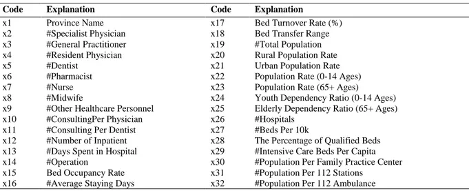
The data set including some health indicators for each province have been provided from a research report of the Ministry of Health of Turkey [7] and given in Table 1. In this report, basic exploratory results have been presented with many measures about health care services according to per province. This report was published in 2016. The latest and up to date data belongs to this year. All variables in this data set are numerical. The clustering methods which are used in this study require numerical data set because of being able to calculate euclidean distances. Therefore, it is appropriate to apply these methods.
It should be noted that İstanbul have the highest scores in all variables scores. Because of having a very special economic and geographic situation, it creates its own cluster in all clustering algorithms and conditions. Additionally, based on the reason which is mentioned in element and variables selection part in this study about including outliers İstanbul has been omitted from the data set. 80 provinces have been evaluated.
Table 1. Variables in Data Set
Code Explanation Code Explanation
x1 x2 x3 x4 x5 x6 x7 x8 x9 x10 x11 x12 x13 x14 x15 x16 Province Name #Specialist Physician #General Practitioner #Resident Physician #Dentist #Pharmacist #Nurse #Midwife
#Other Healthcare Personnel #ConsultingPer Physician #Consulting Per Dentist #Number of Inpatient #Days Spent in Hospital #Operation
Bed Occupancy Rate #Average Staying Days
x17 x18 x19 x20 x21 x22 x23 x24 x25 x26 x27 x28 x29 x30 x31 x32
Bed Turnover Rate (%) Bed Transfer Range #Total Population Rural Population Rate Urban Population Rate Population Rate (0-14 Ages) Population Rate (65+ Ages)
Youth Dependency Ratio (0-14 Ages) Elderly Dependency Ratio (65+ Ages) #Hospitals
#Beds Per 10k
The Percentage of Qualified Beds #Intensive Care Beds Per Capita #Population Per Family Practice Center #Population Per 112 Stations
4.2. The Application of Cluster Analysis
4.2.1. Applying Preprocessing
As mentioned before, preprocessing should be applied to the data set. Firstly PCA has been applied to get orthogonal components and to avoid the high dimensionality. Data dimension has been reduced to nine principal components explaining the variability by % 95. When applying PCA, standardization and centering have been done as default. This approach is utility on reducing negative effects causing both outlier and multicollinearity issues. Multicollinearity can not be existed when apply PCA by the reason of creating orthogonal components. High correlation is foremost indicator about multicollinearity. The correlation between principal components have to be zero. Additionally, outlier analysis process is carried out by using Mahalanobis distance. Based on this process, there is no critical outlier in the data set. The results are given in Appendix B. After preprocessing, aforementioned clustering methods have been applied to these nine principal components by using squared euclid distance via R package program [43].
4.2.2. Assessing Clustering Tendency
In this study, the value of Hopkins statistics is found as 0.2676. This means that the data set is appropriate for clustering.
4.2.3. Using and Comparing Hierarchical Clustering Results
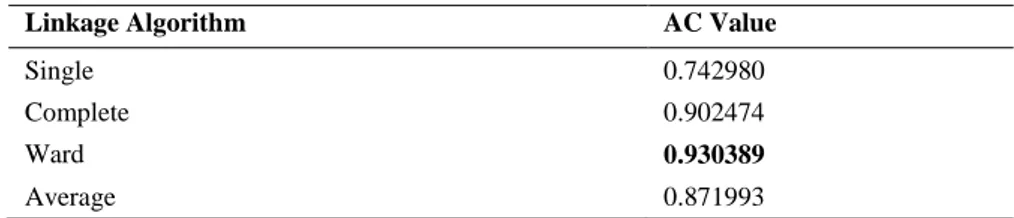
Agglomerative coefficient has been used to compare hierarchical clustering algorithms. The results have been given in Table 2. The maximum AC value has been found as 0.930389 by using Ward linkage. After this step, Ward linkage has been used in hierarchical clustering.
Table 2. Linkage Algorithms and AC Values
Linkage Algorithm AC Value
Single 0.742980
Complete 0.902474
Ward 0.930389
Average 0.871993
Determine The Number of Clusters via Dendrogram in Hierarchical Cluster Analysis
There is no concensus for determining the cutting point in a dendrogram. This point somewhat depends on the researcher and the data set. In other words, there is no definitive answer because of that cluster analysis is essentially an exploratory algorithm. The interpretation and examination of the hierarchical results is context-dependent and often several solutions are equally good from a theoretical point of view. Similar process and logic is conducted in this study.
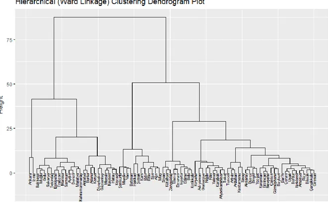
In this study, several solutions are observed and evaulated. In later parts of this study more objective approaches are given for different clustering algorithms but before giving these results it may be useful to discuss several cutting points and results for the dendrogram plot based on Ward linkage which is given in Figure 1. In this plot, if cutting point is taken as 20, there would be five distinct clusters. If this point is placed between 25-40, the number of clusters would be four. Finally after increasing the height to 50, we would have three clusters. Generally speaking, it is observed that the number of clusters which are distinct and clear should be between three and five. In order to making useful interpretations, it is expected that every cluster should have enough observations. It should be considered that including just a few observations may affect the validation of the results.
Figure 1. Hierarchical (Ward Linkage) Clustering Dendrogram Plot 4.2.4. Determining the number of clusters medoids by using cluster validity indices
Determining the number of clusters is the most important part of clustering. Although there is no common sense about this matter, many indices are developed to find and diagnose the ideal number of clusters. In this study, four cluster validity indices and within groups sum of squares (wss) methods have been used. The indices and explainations are given in Table 3. All details, definitions and interpretations about these cluster validity indices have been shared in [36, 44]. One can apply these validity indices to any clustering algorithms such as hierarchical agglomerative clustering, k-means and k-medoids by varying all combinations of number of clusters, distance measures and clustering algorithms [36].
Table 3. The Indices and Explanations
Indice Explanation
1. "Krzanowski&Lai" [45] Maximum value is better 2. "Caliński&Harabasz" [46] Maximum value is better
3. "Hartigan" [23] Max. difference between hierarchy levels of the index 4. "Davies&Bouldin" [47] Minimum value is better
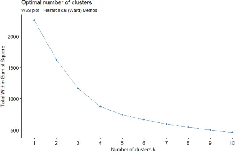
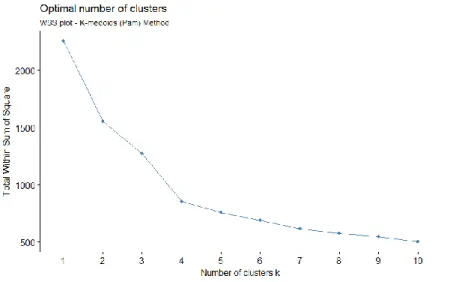
Four indices have been applied to the data set. The findings clearly indicated that there are four distinct and significant clusters are suggested. Also wss plot supports this results. It can be observed in Figure 2. The best values and corresponding suggested number of clusters based on these indices are given in Table 4. All indices values for the range between 2 and 15 clusters is given in Appendix A.
Table 4. Best Indice Values and Suggested Cluster Numbers
Algorithm Best Indice Value Suggested Number of Clusters
KL CH DB Hartigan
Hierarchical 2,35558 39,72372 1,0164 12,8714 4 for All Indices
k-means 6,3407 41,7258 1,0237 12,5809 6 for KL; 4 for CH, DB and Hartigan k-medoids 3,75515 41,53365 1.090984 10.04679 4 for All Indices
One alternative measure for determining the number of clusters is wss plot. This plot gives the change of wss according to the number of clusters. One should look for the location like a bend for the best number of cluster. After this point, it is expected that there will not be a significant change based on the rest of number of clusters. The wss plots drawn for hierarchical clustering, k-means and k-medoids algorithms have been given in Figure 2, Figure 3 and Figure 4. By observing these plots, suggested number of cluster is equal to four.
Figure 2. Wss plot for hierarchical (ward linkage) clustering
Figure 4. Wss plot for k-medoids clustering 4.2.6. Cluster validation
4.2.6.1. Internal validation
Many internal validation measures have been proposed. Similar to determining the number of clusters in a data set, it is hard to say that there is an aggrement for all conditions and purposes. But silhouette width which also preferred in this study, has been used extensively. For interpreting these measures, it should be considered that the silhouette width should be maximized.
Table 5. Comparison between Internal Validation Measure
Clustering Algorithm Validation Measures Score for 4 Clusters Hierarchical k-means k-medoids Silhouette 0.3037 Silhouette 0.3090 Silhouette 0.3033
It can be clearly seen in this table that k-means clustering algorithms slightly predominates to other algorithms under silhouette measure.
4.2.6.2. Stability Measures
Stability measures, a special version of internal measures, which evaluates the consistency of a clustering result by comparing it with the clusters obtained after each column is removed, one at a time. The average of non-overlap (APN), the average distance (AP), the average distance between means (ADM), and the figure of merit (FOM) are the most common and well-known stability measures [30, 48]. While APN measure has the interval [0,1], AD, ADM and FOM changes between zero and infinity. The minimization of each measures provides the best clustering results.
Table 6. Comparison of Stability Validation Measures
Clustering Algorithm Validation Measures Scores for (4) Clusters
Hierarchical APN 0.1838 AD 4.7575 ADM 1.2387 FOM 1.6850 K-means APN 0.1555 AD 4.6206 ADM 0.9253 FOM 1.7056 K-medoids APN 0.2636 AD 4.8410 ADM 1.5204 FOM 1.6853
In reference to Table 6, k-means clustering outperforms the other algorithms under all stability measures except FOM. Under these measures, it has the lowest values. Hierarchical clustering has been found as best for just under FOM measure value. Last of all, k-means has been found as the best algorithm for this data set according to the majority of stability measures.
5. RESULTS
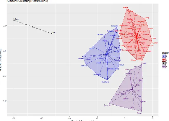
As mentioned in the previous sections of this study, four meaningful and significant clusters have been found by using some cluster validity indices. The results of both internal validation and stability measures indicate that k-means clustering algorithms is the most suitable for this data set. Therefore, it has been applied to the data set for k=4. Because of high dimensions, first two principal components has been used to observed the results visually. The graph is given in Figure 5. Cluster informations such as size and members can be seen in Table 7. Finally cluster centers for original scaled data set are given in Table 8. Cluster centers correspond to the vector fo means of each variable in a cluster.
Table 7. Clusters and Members of Hierarchical Clustering
Cluster {Size} Members Cluster {Size} Members
Cluster 1 {2} Ankara İzmir Cluster 2 {22}
Adana Antalya Aydın Balıkesir Bursa Denizli Diyarbakır Eskişehir Gaziantep Hatay Mersin Kayseri Kocaeli Konya Malatya Manisa Kahramanmaraş Muğla Sakarya Samsun Tekirdağ Trabzon Cluster 3 {41} Afyonkarahisar Amasya Artvin Bilecik Bolu Burdur Çanakkale Çankırı Çorum Edirne Elazığ Erzincan Erzurum Giresun Gümüşhane Isparta Kars Kastamonu Kırklareli Kırşehir Kütahya Nevşehir Niğde Ordu Rize Sinop Sivas Tokat Tunceli Uşak Yozgat Zonguldak Bayburt Karaman Kırıkkale Bartın Ardahan Yalova Karabük Kilis Düzce Cluster 4 {15} Adıyaman Ağrı Bingöl Bitlis Hakkari Mardin Muş Siirt Şanlıurfa Van Aksaray Batman Şırnak Iğdır Osmaniye
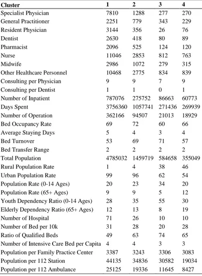
Table 8. Cluster Centers with Original Scale
Cluster 1 2 3 4 Specialist Physician 7810 1288 277 270 General Practitioner 2251 779 343 229 Resident Physician 3144 356 26 76 Dentist 2630 418 80 89 Pharmacist 2096 525 124 120 Nurse 11046 2853 812 763 Midwife 2986 1072 279 315
Other Healthcare Personnel 10468 2775 834 839
Consulting per Physician 9 9 7 9
Consulting per Dentist 1 1 0 1
Number of Inpatient 787076 275752 86663 60773 Days Spent 3756360 1057741 271436 269939 Number of Operation 362166 94507 21013 18929
Bed Occupancy Rate 69 72 60 66
Average Staying Days 5 4 3 4
Bed Turnover 53 69 71 57
Bed Transfer Range 2 2 2 2
Total Population 4785032 1459719 584658 355049
Rural Population Rate 1 4 38 46
Urban Population Rate 99 96 62 54 Population Rate (0-14 Ages) 20 23 34 20 Population Rate (65+ Ages) 9 9 5 12 Youth Dependency Ratio (0-14 Ages) 28 35 55 30 Elderly Dependency Ratio (65+ Ages) 12 13 8 19
Number of Hospital 71 26 10 10
Number of Bed per 10k 31 28 20 28 Ratio of Qualified Beds 49 63 74 65 Number of Intensive Care Bed per Capita 4 4 3 3 Population per Family Practice Center 3387 3243 3306 3083 Population per 112 Station 44135 34836 30582 19034 Population per 112 Ambulance 25125 19336 11645 8427
6. CONCLUSIONS AND DISCUSSIONS
This study set out to get some useful insights about accessing health care services between Turkey provinces. The results show that four clusters exist in Turkey provinces in terms of accessing these services. Cluster analysis revealed that citizens living in different provinces have not equal opportunities to get enough health services.
Despite cluster analysis exploratory nature, this study offers some insights into issues about health rights. In general, it seems that all the members of Cluster 1 & Cluster 2 are metropolises in Turkey. 24 of 30 metropolises in Turkey constitute these two clusters. It can be said that the quality of services is proportional with the development level of provinces. Mardin, Van, Şanlıurfa, Erzurum and Ordu provinces are exceptional. Although each of these provinces is a metropolis, they are below in terms of health service opportunities compared with the other metropolises.
The empirical findings in this study provide a new understanding of the levels of health services in Turkey. When examining the centers of clusters in Table 8, clustering results can be categorized into first level for Cluster 1 and similarly fourth level for Cluster 4. Lower level means better health services. Specificially most of members in Cluster 4 are located in the eastern and the southeastern anatolia regions. It is known that there are some lacks of opportunities because of regional issues in these regions. While most of the provinces in cluster 1 & 2 are located in the west of Turkey, almost all of the eastern provinces which have lower or lowest health indicator scores are included in cluster 4. The third cluster results have a moderate position between these two separations according to the cluster centers.
Consequently, some suggestions related with health services may be introduced. It would be useful to look for the ways which can balance these disparities on health services between provinces. The east provinces should be funded to move forward the economic levels of these provinces. By motivating civil society organizations and academicians to do research on this matter may be beneficial and provide better insights to resolve the health sector problems.
REFERENCES
[1] WHO. Basic Documents, Forty-Third Edition, World Health Organization 2001; apps.who.int/gb/bd/. (Last Access Date: 07/04/2018)
[2] Pala K. Türkiye İçin Nasıl Bir Sağlık Reformu? 2005. Bursa Nilüfer Belediyesi, Bursa.
[3] TTB. Sağlıkta gündem: Herkese eşit fırsat mı? Serbest piyasa egemenliği mi? Sağlık Bakanlığı Ulusal Sağlık Politikası Taslak Dökümanı Değerlendirme Raporu. Türk Tabipleri Birliği 1992; Ankara.
[4] Çınaroğlu S, Avcı K. İstatistiki bölge birimlerinin seçilen sağlık göstergeleri bakımından kümelenmesi. Hacettepe Sağlık İdaresi Dergisi 2014; 17.2.
[5] Tekin B. Temel sağlik göstergeleri açısından Türkiye'deki illerin gruplandırılması: Bir kümeleme analizi uygulaması. Çankırı Karatekin Üniversitesi İktisadi ve İdari Bilimler Fakültesi Dergisi 2015; 5(2): 389.
[6] Taban S. Türkiye'de sağlık ve ekonomik büyüme arasındaki nedensellik ilişkisi. Sosyoekonomi 2006; 4.4.
[7] T.C. Sağlık Bakanlığı, Sağlık İstatistikleri Yıllığı 2016; Ankara. https://dosyasb.saglik.gov.tr/Eklenti/13183,sy2016turkcepdf.pdf?0 (Son Erişim Tarihi: 07/04/2018)
[8] Hamarat B. Türkiye’de sağlık açısından homojen il gruplarının belirlenmesine ilişkin istatiksel bir yaklaşım. Y. Lisans Tezi, Anadolu Üniversitesi, Eskişehir, 1998.
[9] Çilan ÇA, Demirhan, A. Türkiye’nin illere göre sosyoekonomik yapısının çok boyutlu ölçekleme tekniği ve kümeleme analizi ile incelenmesi. Yönetim Dergisi 2002; 42: 39-50.
[10] Albayrak AS, Kalaycı Ş, Karataş A. Türkiye'de coğrafi bölgelere göre illerin sosyoekonomik gelişmişlik düzeylerinin temel bileşenler analiziyle incelenmesi. Süleyman Demirel Üniversitesi İktisadi ve İdari Bilimler Fakültesi Dergisi 2004; 9:2.
[11] Karabulut M, Gürbüz M, Sandal EK. Hiyerarşik kluster (küme) tekniği kullanılarak Türkiye’de illerin sosyo-ekonomik benzerliklerinin analizi. Coğrafi Bilimler Dergisi 2004; 2.2: 65-78. [12] Kaygısız Z, Saraçlı S, Dokuzlar KU. İllerin gelişmişlik düzeyini etkileyen faktörlerin path analizi
ve kümeleme analizi ile incelenmesi. VII. Ulusal Ekonometri ve İstatistik Sempozyumu; 2005. İstanbul Üniversitesi, İstanbul, Türkiye.
[13] Filiz Z. İllerin sosyo-ekonomik düzeylerine göre gruplandırılmasında farklı yaklaşımlar. Eskişehir Osmangazi Üniversitesi Sosyal Bilimler Dergisi 2014; 6.1: 77-100.
[14] Altıparmak A. Sosyo-ekonomik göstergeler açısından illerin gelişmişlik düzeyinin karşılaştırmalı analizi. Erciyes Üniversitesi İktisadi ve İdari Bilimler Fakültesi Dergisi 2005; 24.
[15] Taner T, Erilli A, Yüksel Ö, Yolcu U. İllerin sosyoekonomik verilere dayanarak bulanık kümeleme analizi ile sınıflandırılması. Physical Sciences 2009; 4(1): 1-11.
[16] Yılancı AGV. Bulanık kümeleme analizi ile Türkiye'deki illerin sosyoekonomik açıdan sınıflandırılması. Süleyman Demirel Üniversitesi İktisadi ve İdari Bilimler Fakültesi Dergisi 2010; 15(3).
[17] Yıldız EB, Sivri U, Berber M. Türkiye’de illerin sosyo-ekonomik gelişmişlik sıralaması. Uluslararası Bölgesel Kalkınma Sempozyumu; 2010. Bozok Üniversitesi, Yozgat, Türkiye. [18] Çemrek F. Türkiye’deki illerin gelir ve refah düzeyi değişkenleri arasındaki ilişkinin kanonik
korelasyon analizi ile incelenmesi. Eskişehir Osmangazi Üniversitesi İktisadi ve İdari Bilimler Dergisi 2012; 7.2.
[19] Çelik Ş. Kümeleme analizi ile sağlık göstergelerine göre Türkiye’deki illerin sınıflandırılması. Doğuş Üniversitesi Dergisi 2013; 14 (2): 175-194
[20] Rencher AC. Methods of Multivariate Analysis. (Vol. 492), New York, NY, USA: Wiley, 2002 [21] Sharma S. Applied Multivariate Techniques. New York, NY, USA: Wiley, 1995.
[22] Yıldırım H. The usage of dissimilarity and similarity measures in statistics. Msc, Çukurova University, Adana, Turkey, 2015.
[23] Hartigan J. Clustering algorithms. New York, NY, USA: Wiley, 1975.
[24] Yan M. Methods of determining the number of clusters in a data set and an clustering criterion. Ph.D, Institute and State University, Blacksburg, Virginia, 2005.
[25] Mo'oamin MR, Hamad BS. Using cluster analysis and discriminant analysis methods in classification with application on standard of living family in palestinian areas. International Journal of Statistics and Applications 2015; 5.5: 213-222.
[26] Everitt BS, Landau S, Leese M, Stahl D. Cluster Analysis. 5th Edition. New York, NY, USA: Wiley, 2011.
[27] Choi SS, Cha SH, Tappert, CC. A survey of binary similarity and distance measures. Journal of Systemics, Cybernetics and Informatics 2010; 8.1: 43-48.
[28] Cha SH. Comprehensive survey on distance/similarity measures between probability density functions. City 2007; 1.2: 1.
[29] Lawson RG, Jurs PC. New index for clustering tendency and its application to chemical problems. Journal of Chemical Information and Computer Sciences 1990; 30.1: 36-41.
[30] Kassambara A. Practical guide to cluster analysis in R: Unsupervised machine learning. (Vol. 1). Sthda, 2017.
[31] Banerjee A, Dave RN. Validating clusters using the Hopkins statistic. In: Fuzzy Systems, 2004. Proceedings. 2004 IEEE International Conference On. IEEE; 2004; pp. 149-153.
[32] Dubes RC, Jain AK. Algorithms for clustering data. Prentice Hall, Englewood Cliffs, 1988 [33] Tan PN, Steinbach M, Kumar V. Introduction to data mining. 1st. Boston, Pearson Addison
Wesley, 2005.
[34] Beglinger LJ, Smith TH. A review of subtyping in autism and proposed dimensional classification model. Journal of Autism and Developmental Disorders 2001; 31:4: 411-422. [35] Sokal RR. A statistical method for evaluating systematic relationship. University of Kansas
Science Bulletin 1958; 28: 1409-1438.
[36] Charrad M, Ghazzali BV, Niknafs A. NbClust: An R package for determining the relevant number of clusters in a data set. Journal of Statistical Software 2014; 61(6): 1-36.
[37] Sørensen T. A method of establishing groups of equal amplitude in plant sociology based on similarity of species and its application to analyses of the vegetation on danish commons. Biol. Skr 1948; 5:1: 34.
[38] Ward JR, Joe H. Hierarchical grouping to optimize an objective function. Journal of The American Statistical Association 1963; 58.301: 236-244.
[39] Kaufman L, Rousseeuw PJ. Finding groups in data: An introduction to cluster analysis. New York, NY, USA: Wiley 1990.
[40] Maechler M, Rousseeuw P, Struyf A, Hubert M, Hornik K. Cluster: Cluster analysis basics and extensions. R Package Version 2012; 1.2: 56.
[41] Hartigan JA, Wong MA. Algorithm as 136: A k-means clustering algorithm. Journal Of The Royal Statistical Society. Series C (Applied Statistics) 1979; 28.1: 100-108.
[42] Ansari Z, Azeeem MF, Ahmet W, Babu AV. Quantitative evaluation of performance and validity indices for clustering the web navigational sessions. CoRR 2015. abs/1507.03340
[43] R Core Team. R: A language and environment for statistical computing. R Foundation for Statistical Computing, Vienna, Austria. Url http://www.r-project.org/.
[44] Halkidi M, Vazirgiannis M, Batistakis Y. Quality scheme assessment in the clustering process. In: European Conference On Principles of Data Mining And Knowledge Discovery. Springer, Berlin, Heidelberg 2000; 265-276.
[45] Krzanowski WJ, Lai YT. A criterion for determining the number of groups in a data set using sum-of-squares clustering. Biometrics 1988; 23-34.
[46] Caliński T, Harabasz, J. A dendrite method for cluster analysis. Communications in Statistics-Theory and Methods 1974; 3.1: 1-27.
[47] Davies DL, Bouldin, DW. A cluster separation measure. IEEE Transactions on Pattern Analysis and Machine Intelligence 1979; 2: 224-227.
[48] Brock G, Pihur V, Datta S, Datta S. ClValid: An R package for cluster validation. Journal of Statistical Software 2011.
APPENDIXES
Appendix A. Cluster Validity Indices and Values for Different Cluster Numbers
k KL CH DB Hartigan Hierarchical 2 0,70840 30,28279 1,4976 17,7368 3 1,35100 36,13868 1,2869 37,3416 4 2,35558 39,72372 1,0164 12,8714 5 1,70037 37,86064 1,0436 9,0922 6 1,00609 35,31188 1,1232 8,8833 7 1,37824 33,83445 1,2054 6,3751 8 0,96824 32,23034 1,2479 7,8977 9 1,05587 31,23317 1,2276 4,2481 10 0,97121 30,51831 1,2153 4,5164 11 1,42774 30,19718 1,207 6,0828 12 0,93620 29,45296 1,1688 7,2106 13 1,28897 29,04177 1,0656 3,9248 14 0,97352 28,41967 1,0556 4,4818 15 1,14363 27,99481 1,0834 3,6343 k-means 2 1,9868 35,1855 1,4444 18,8622 3 0,4062 30,8772 1,3355 36,1098 4 4,127 41,7258 1,0237 12,5809 5 1,4489 39,0987 1,2026 9,4638 6 1,053 36,6237 1,1769 8,7564 7 1,7294 35,1096 1,2761 6,045 8 0,663 32,9913 1,2643 7,5358 9 6,3407 32,3748 1,2947 2,9643 10 0,2411 29,8815 1,2594 5,3243 11 0,9322 29,0503 1,2165 5,5054 12 1,5998 28,5965 1,1389 3,9698 13 1,8682 27,6618 1,1334 2,7194 14 0,5522 26,3798 1,2089 3,6847 15 2,6077 25,7304 1,2288 2,1162 Pam 2 0,95778 35,05710 1.356483 17.73934 3 1,48149 39,56545 1.268066 38.03599
4 3,75515 41,53365 1.090984 10.04679 5 1,43605 36,95039 1.392098 7.300226 6 3,60705 33,39535 1.619447 8.998696 7 0,14455 29,70813 1.595953 4.944107 8 2,40677 29,63178 1.341798 4.105301 9 0,74311 28,05652 1.271905 6.84791 10 0,90102 27,31365 1.248767 3.356672 11 1,39389 27,05249 1.186856 6.268196 12 0,63082 26,43769 1.154338 5.893722 13 3,47531 26,93201 1.131464 5.628311 14 0,49406 25,82170 1.162242 4.284865 15 1,05444 25,59464 1.191507 4.930126
Appendix B. Mahalanobis distances for each province
Province Mahalanobis Distance Province Mahalanobis Distance
Adana 10,2129 Konya 3,7026 Adıyaman 5,2329 Kütahya 9,2282 Afyonkarahisar 4,4161 Malatya 10,0358 Ağrı 8,9538 Manisa 5,4698 Amasya 8,8500 Kahramanmaraş 2,7034 Ankara 54,8602 Mardin 8,6804 Antalya 7,2251 Muğla 8,3022 Artvin 8,4693 Muş 9,1464 Aydın 3,7180 Nevşehir 6,4781 Balıkesir 6,6970 Niğde 3,7277 Bilecik 9,9808 Ordu 4,5444 Bingöl 7,7556 Rize 8,1777 Bitlis 5,3094 Sakarya 6,9663 Bolu 21,8144 Samsun 6,7815 Burdur 3,1345 Siirt 9,4724 Bursa 6,7857 Sinop 9,4180 Çanakkale 6,5815 Sivas 7,4770 Çankırı 8,6932 Tekirdağ 7,8448 Çorum 1,9543 Tokat 2,4917 Denizli 3,5163 Trabzon 5,5336 Diyarbakır 7,8941 Tunceli 12,3993 Edirne 8,6321 Şanlıurfa 11,4735 Elazığ 11,2747 Uşak 6,4577 Erzincan 2,2941 Van 8,1625 Erzurum 15,7843 Yozgat 7,7576 Eskişehir 7,1936 Zonguldak 2,3600 Gaziantep 6,4901 Aksaray 9,4581 Giresun 8,9365 Bayburt 17,2620 Gümüşhane 7,5101 Karaman 4,6981 Hakkari 22,1107 Kırıkkale 12,2969 Hatay 3,7345 Batman 7,0845 Isparta 11,2588 Şırnak 13,1138 Mersin 4,7657 Bartın 14,9656 İzmir 17,8494 Ardahan 8,8290 Kars 7,3250 Iğdır 8,3280 Kastamonu 12,3569 Yalova 13,7395 Kayseri 5,4351 Karabük 7,5364 Kırklareli 8,3192 Kilis 15,0111 Kırşehir 6,6924 Osmaniye 12,1420 Kocaeli 5,9578 Düzce 5,7668 Threshold Value = 𝜒2 (0,001;31) = 61.1