Nonnull curves with constant weighted curvature in Lorentz-Minkowski plane with density

© TÜBİTAK

doi:10.3906/mat-1908-2 h t t p : / / j o u r n a l s . t u b i t a k . g o v . t r / m a t h /

Research Article

Nonnull Curves with Constant Weighted Curvature in Lorentz-Minkowski Plane

with Density

Mustafa ALTIN1,∗_{,, Ahmet KAZAN}2 _{,, Hacı Bayram KARADAĞ}3 _, 1_{Technical Sciences Vocational School, Bingöl University, Bingöl, Turkey}

2_{Department of Computer Technologies, Doğanşehir Vahap Küçük Vocational School of Higher Education,}

Malatya Turgut Özal University, Malatya, Turkey

3_{Department of Mathematics, Faculty of Arts and Sciences, İnönü University, Malatya, Turkey}

Received: 01.08.2019 • Accepted/Published Online: 21.02.2020 • Final Version: 17.03.2020

Abstract: In this paper, the parametric expressions of spacelike and timelike curves with constant weighted curvature

for some cases of a and b in Lorentz-Minkowski plane with density eax+by _{are obtained.}

Key words: Lorentz-Minkowski plane, plane with density, weighted curvature

1. Introduction

In 2003, Gromov has introduced the notions of weighted mean curvature of an n -dimensional hypersurface and weighted curvature of a curve on manifolds with density as

Hφ= H− 1 n− 1 dφ dη and κφ= κ− dφ dN,

respectively [5]. Here, H is the mean curvature and η is the normal vector field of an n -dimensional hypersur-face; κ is the curvature and N is the normal vector of the curve.

After these definitions, the differential geometry of the curves and hypersurfaces on manifolds with density in Euclidean, Minkowski and Galilean spaces has been started to be an important topic for geometers, physicists, economists and etc. For instance, in 2006 the authors have defined the weighted Gaussian curvature and they have given a generalization of Gauss-Bonnet formula for 2-dimensional differentiable manifold with density in [4]. In [11–13], F.Morgan has studied the manifolds with density, provided the generalizations of theorems of Myers and others to Riemannian manifolds with density and studied the Perelman’s proof of the Poincare conjecture, respectively.

The classification of constant weighted curvature curves in a plane with a log-linear density has been done in [7] and some other results, such as Fenchel’s type theorem for the class of simple, closed, convex curves and the fact ”the plane with density ex _{contains no isoperimetric region” have been proved in [14]. In [10],}

Lopez has studied the minimal surfaces in Euclidean 3-space with a log-linear density φ(x, y, z) = αx + βy + γz, where α, β and γ are real numbers not all-zero. Also, Belarbi et al. have studied the surfaces in R3 _with

density and they have given some results in a Riemannian manifold M with density in [1] and [2], respectively.

∗_{Correspondence: maltin@bingol.edu.tr}

2010 AMS Mathematics Subject Classification: 53A35, 53B30.

Furthermore, ruled and translation minimal surfaces in R3 _{with density e}z_{; helicoidal surfaces in R}3

with density e−x2−y2 and weighted minimal affine translation surfaces in Euclidean space with density have been studied in [6,18, 19], respectively. Also, some types of surfaces have been studied by geometers in other spaces such as Minkowski 3-space and Galilean 3-space with density. For instance, a helicoidal surface of type I+

with prescribed weighted mean curvature and Gaussian curvature in Minkowski 3-space and weighted minimal translation surfaces in Minkowski 3-space with density ez _{have been constructed in [15] and [16], respectively. In}

[17], weighted minimal translation surfaces in the Galilean 3-space with log-linear density has been classified and in [8], weighted minimal and weighted flat surfaces of revolution in Galilean 3-space with density eax2+by2+cz2

have been investigated.

Now, we’ll recall some basic notions about curves in Lorentz-Minkowski plane.

Let L2 _{be Lorentz-Minkowski plane defined as a space to be usual 2-dimensional vector space consisting}

of vectors {(x0_{, x}1_{) : x}0_{, x}1_{∈ R} but with a linear connection ∇ corresponding to its Minkowski metric g given}

by g(x, y) =−x0_y0_{+ x}1_y1_{. Here, there are three categories of vector fields, namely,} spacelike if g(X, X) > 0 or X = 0 ,

timelike if g(X, X) < 0 ,

lightlike (null) if g(X, X) = 0 , X ̸= 0. In general, the type into which a given vector field X falls is

called the causal character of X .

For a curve α = (α1, α2) : I ⊆ R −→ R2 in Lorentz-Minkowski plane, where I is some interval in R,

it is said that α = α(t) is spacelike (resp. timelike or lightlike) if the tangent vector α′(t) is spacelike (resp. timelike or lightlike) for ∀t ∈ I . Now, let α = (α1, α2) be a spacelike (or timelike) curve which is parametrized

by arc-length; i.e. g(α′(u), α′(u)) = 1 (or g(α′(u), α′(u)) = −1), for ∀u ∈ I . For the curve α = (α1, α2),

the tangent vector of it is T = α′ = (α′₁, α′₂) and we can choose the corresponding normal vector of α as

N = (α′₂, α′₁) . Here, it is obvious that the tangent vector T and normal vector N of α have different causal

characters. If we take g(T, T ) = ϵ , then we have g(N, N ) = −ϵ and the curve α is spacelike for ϵ = 1 and timelike for ϵ =−1. Also, the curvature of α is the function of κ = κ(u) and it is given by

T′(u) = κ(u)N (u), (1.1)

where

κ(u) =−ϵg(T′(u), N (u)) = ϵ(x′′(u)y′(u)− x′(u)y′′(u)). (1.2)

Furthermore, we have

N′(u) = κ(u)T (u). (1.3)

For more details about Frenet dihedron of a curve in Lorentz-Minkowski plane, we refer to [3] and [9].

In the present study, we’ll deal with spacelike and timelike curves in Lorentz-Minkowski plane with density and the aim of this study is to investigate the spacelike and timelike curves with constant weighted curvature in Lorentz-Minkowski plane with density eax+by_.

2. Spacelike Curves with Constant Weighted Curvature in Lorentz-Minkowski Plane with Density

eax+by

In this section, we obtain the weighted curvature κφ of a spacelike curve α in Lorentz-Minkowski plane with

zero constants a and b.

The weighted curvature κφ(u) of a spacelike curve α(u) = (x(u), y(u)) with arc-length paremeter in

Lorentz-Minkowski plane with density eax+by _{is obtained as}

κφ(u) = κ(u)− ⟨∇φ, N(u)⟩ = x′′(u)y′(u)− x′(u)y′′(u) + ay′(u)− bx′(u), (2.1)

where N (u) = (y′(u), x′(u)) . Since α(u) = (x(u), y(u)) is a spacelike curve with arc-length papameter, we can take

x′(u) = sinh(f (u)),

y′(u) = cosh(f (u)). (2.2)

So, from (2.1) and (2.2), the constant weighted curvature κφ(u) can be written as

κφ(u) = a cosh(f (u))− b sinh(f(u)) + f′(u) = λ, (2.3)

where λ∈ R.

Now, let us obtain the spacelike curves with constant weighted curvature λ according to some cases of constants a and b.

2.1. The Case of ” a = b”

In this case, the equation (2.3) can be rewritten as

a cosh(f (u))− a sinh(f(u)) + f′(u) = λ. (2.4)

Using the definition of the hyperbolic functions in (2.4), we have

f′(u)ef (u)= λef (u)− a. (2.5)

Now, we can find the spacelike curves by solving the equation (2.5) according to cases of constant λ.

2.1.1. Solving equation (2.5) for λ = 0 :

Taking λ = 0 in (2.5), we have

ef (u)f′(u) =−a (2.6)

and from (2.6), we get

d(ef (u)) =−adu. (2.7)

By integrating both sides of (2.7), we obtain that

ef (u) = k1− au, k1∈ R. (2.8)

Hence, from (2.2) and (2.8), we have

x′(u) = (k1−au)2−1 2(k1−au) , y′(u) = (k1−au)2+1

2(k1−au) .

(2.9) Thus, from (2.9), we can give the following Theorem:

Theorem 2.1 The spacelike curve α(u) with vanishing weighted curvature in Lorentz-Minkowski plane with

density ea(x+y) _is

α(u) = (

au(2k1− au) + 2 ln(k1− au)

4a + k2,

au(2k1− au) − 2 ln(k1− au)

4a + k3

)

, (2.10)

where k1− au > 0 and ki∈ R, i = 1, 2, 3.

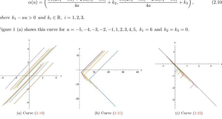
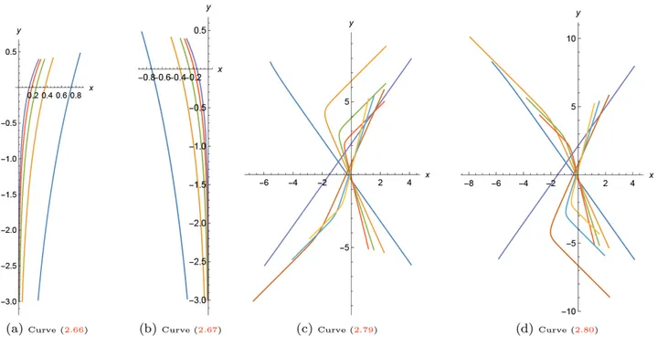
Figure 1 (a) shows this curve for a =−5, −4, −3, −2, −1, 1, 2, 3, 4, 5, k1= 6 and k2= k3= 0 .

Figure 1. The spacelike curves with constant weighted curvature in Lorentz-Minkowski plane with density ea(x+y) _for different values of constant a .

2.1.2. Solving equation (2.5) for λ̸= 0:

Firstly, let’s take f′(u) = 0 . From equation (2.5), we have ef (u)= a

λ. (2.11)

So, from (2.2) and (2.11), we get

x′(u) = a2_2aλ−λ2,

y′(u) = a2_2aλ+λ2. (2.12)

Now, let us take f′(u)̸= 0. Then from (2.5), we get f′(u)ef (u) ef (u)−a λ = λ (2.13) and d(ef (u)) ef (u)₋a λ = λdu. (2.14)

By integrating both sides of (2.14), we have  ef (u)₋a λ   = eλu+k6_{. (2.15)}

From (2.15), we can write

ef (u)= a λ+ e λu+k6 _(2.16) or ef (u) = a λ− e λu+k6_{. (2.17)}

Using (2.16) and (2.17) in (2.2), then we have

x′(u) = a λ+eλu+k6−a 1 λ+eλu+k6 2 , y′(u) = a λ+eλu+k6+a 1 λ+eλu+k6 2 (2.18) and x′(u) = a λ−eλu+k6− 1 a λ −eλu+k6 2 , y′(u) = a λ−eλu+k6+ 1 a λ −eλu+k6 2 , (2.19)

respectively. Hence, from (2.12), (2.18) and (2.19), we can state the following Theorem:

Theorem 2.2 The spacelike curves with non-zero constant weighted curvature κφ= λ in Lorentz-Minkowski

plane with density ea(x+y) _are

i) the straight line of

α(u) = ( a2_{− λ}2 2aλ u + k4, a2_{+ λ}2 2aλ u + k5 ) , (2.20) whose slope is a2+λ2

a2_−λ2. In the case of a = λ , the slope of lines is ∞, i.e. the lines are vertical, where

a λ > 0 and ki∈ R, i = 4, 5; ii) α(u) = ( au + eλu+k6 2λ + lnae−λu+ λek6 2a + k7, au + eλu+k6 2λ − lnae−λu+ λek6 2a + k8 ) , (2.21) where ae−λu λ >−e k6 and k i∈ R, i = 6, 7, 8 or iii) α(u) = ( au− eλu+k6 2λ + lnae−λu− λek6 2a + k9, au− eλu+k6 2λ − lnae−λu− λek6 2a + k10 ) , (2.22) where ae−λu λ > e k6 and k i∈ R, i = 6, 9, 10.

Figure 1 (b) shows the curve (2.21) for λ = 10, a = 1, 2, 3, 4, 5, k6 = 11 and k7 = k8 = 0 and Figure 1 (c)

2.2. The Case of ” a̸= 0, b = 0”

In this case, the equation (2.3) can be rewritten as

a cosh(f (u)) + f′(u) = λ. (2.23)

From (2.23), we have 2f′(u)ef (u)= a [ λ2 a2 − 1 − ( ef (u)−λ a )2] . (2.24)

Now, we can obtain the spacelike curves by solving the equation (2.24) according to cases of constant λ.

2.2.1. Solving equation (2.24) for λ = a:

Firstly, let’s take f′(u) = 0 . From equation (2.24), we have

ef (u) = 1. (2.25)

So, from (2.2) and (2.25), we get

x(u) = c1,

y(u) = u + c2, c1, c2∈ R. (2.26)

Now, let us take f′(u)̸= 0 in equation (2.24). Then, we have 2f′(u)ef (u) ( ef (u)− 1)2 =−a and so, 2d(ef (u)₎ ( ef (u)_{− 1})2 =−adu. (2.27)

By integrating both sides of (2.27), we get

ef (u)= 2

au− c3

+ 1. (2.28)

So, from (2.2) and (2.28)

x′(u) = ( 2 au−c3+1)2−1 2( 2 au−c3+1) , y′(u) = ( 2 au_−c3+1) 2₊₁ 2( 2 au−c3+1) . (2.29)

Thus, from (2.2.1) and (2.29), we have

Theorem 2.3 The spacelike curves α(u) with constant weighted curvature κφ= λ in Lorentz-Minkowski plane

with density eax _{for λ = a are}

i) the straight line of

whose slope of lines is ∞, i.e. the lines are vertical and ci ∈ R, i = 1, 2 or ii) α(u) =  ln((au − c3)(au− c3+ 2)) a + c4, au + ln ( au_−c3 au−c3+2 ) a + c5   , (2.31) where au− c3∈ R − [−2, 0] and ci∈ R, i = 3, 4, 5.

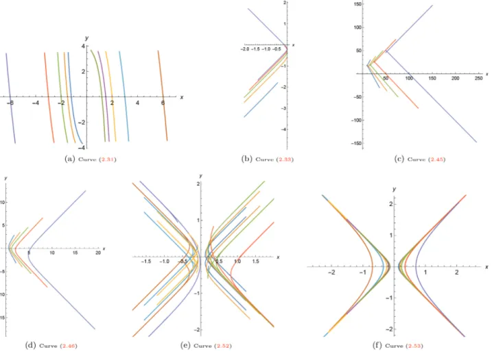
Figure 2 (a) shows the curve (2.31) for λ = a =−5, −4, −3, −2, −1, 1, 2, 3, 4, 5, c3= 21 and c4= c5= 0 .

Figure 2. The spacelike curves with constant weighted curvature in Lorentz-Minkowski plane with density eax _for different values of constant a .

2.2.2. Solving equation (2.24) for λ =−a:

With similar procedure in the case of λ = a , one can easily find that x′(u) = ( 2 au−c6−1)2−1 2( 2 au−c6−1) , y′(u) = ( 2 au−c6−1)2+1 2( 2 au−c6−1) . (2.32)

From (2.32), we can state the following Theorem:

Theorem 2.4 The spacelike curve α(u) with constant weighted curvature κφ= λ in Lorentz-Minkowski plane

with density eax _{for λ =−a is}

α(u) =  ln ((au − c6)(2 + c6− au)) a + c7,−u + ln( au−c6 2+c6−au ) a + c8   , (2.33) where au− c6∈ (0, 2) and ci∈ R, i = 6, 7, 8.

Figure 2 (b) shows this curve for λ =−a = −5, −4, −3, −2, −1, c6= c7= c8= 0.

2.2.3. Solving equation (2.24) for λ a > 1 :

Firstly, let us assume that f′(u) = 0 . From (2.24), we have

a [( ef (u)−λ a )2 + 1−λ 2 a2 ] = 0 and so, ef (u) =λ a ± √ (λ a) 2− 1. _(2.34)

Thus, from (2.2) and (2.34), we have

x′(u) = λ a± √ (λ a)2−1−_λ 1 a ± √ ( λ_a)2−1 2 , y′(u) = λ a± √ (λ a)2−1+ 1 λ a ± √ ( λ_a)2−1 2 . (2.35)

Now, let us take f′(u)̸= 0. From equation (2.24), we get 2f′(u)ef (u) ( ef (u)₋λ a )2 + 1−λ_a22 =−a ⇒   1 ef (u)₋λ a − √ λ2 a2 − 1 − 1 ef (u)₋λ a + √ λ2 a2 − 1   f_√′(u)ef (u) λ2 a2 − 1 =−a ⇒   1 ef (u)₋λ a − √ λ2 a2 − 1 − 1 ef (u)₋λ a + √ λ2 a2 − 1 

 d(ef (u)_{) =−a}

√ λ2

By integrating both sides of (2.36), we get    ef (u)₋λ a − √ λ2 a2 − 1 ef (u)−λ a + √ λ2 a2 − 1   = e−a √ λ2 a2−1u+c11. (2.37)

Thus, we can write

ef (u)−λ_a − √ λ2 a2 − 1 ef (u)−λ a + √ λ2 a2 − 1 = e−a √ λ2 a2−1u+c11 (2.38) or ef (u)₋λ a − √ λ2 a2 − 1 ef (u)−λ a + √ λ2 a2 − 1 =−e−a √ λ2 a2−1u+c11_. (2.39)

From (2.38) and (2.39), we have

ef (u)= (√ λ2 a2 − 1 − λ a ) e−a √ λ2 a2−1u+c11+λ a + √ λ2 a2 − 1 ( 1− e−a √ λ2 a2−1u+c11 ) (2.40) and ef (u) = ( λ a − √ λ2 a2 − 1 ) e−a √ λ2 a2−1u+c11₊λ a + √ λ2 a2 − 1 ( 1 + e−a √ λ2 a2−1u+c11 ) , (2.41)

respectively. So, from (2.2) and (2.40), we obtain

x′(u) = ( (m−n)eamu+c11 +n+m (1−eamu+c11) )2 −1 2 ( (m−n)eamu+c11 +n+m (1−eamu+c11) ) , y′(u) = ( (m−n)eamu+c11 +n+m (1−eamu+c11) )2 +1 2 ( (m−n)eamu+c11 +n+m (1−eamu+c11) ) (2.42)

and from (2.2) and (2.41),

x′(u) = ( (n−m)e−amu+c11 +n+m (1+e−amu+c11) )2 −1 2 ( (n−m)e−amu+c11 +n+m (1+e−amu+c11) ) , y′(u) = ( (n−m)e−amu+c11 +n+m (1+e−amu+c11) )2 +1 2 ( (n−m)e−amu+c11 +n+m (1+e−amu+c11) ) , (2.43) where m = √ λ2 a2 − 1 and n = λ

Theorem 2.5 The spacelike curves with constant weighted curvature κφ= λ in Lorentz-Minkowski plane with

density eax _for λ

a > 1 are

i) the straight line of

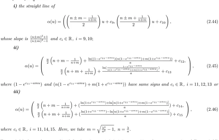
α(u) = (( n± m − 1 n±m 2 ) u + c9, ( n± m + 1 n±m 2 ) u + c10 ) , (2.44)

whose slope is (n_(n±m)_±m)22+1₋₁ and ci∈ R, i = 9, 10;

ii) α(u) =    u 2 ( n + m−_n+m1 )

+ln((1−ec11−amu)(n(1−ec11−amu_a )+m(1+ec11−amu)) + c12, u 2 ( n + m + _n+m1 ) + ln( 1−ec11−amu n(1−ec11−amu)+m(1+ec11−amu)) a + c13    , (2.45)

where (1− ec11−amu_{) and (n(1}− ec11−amu_{) + m(1 + e}c11−amu_{)) have same signs and c}

i∈ R, i = 11, 12, 13 or iii) α(u) =   u 2 ( n + m−_n+m1 )

+ (ln(1+ec11−amu)+ln|n(1+ec11−amu_a )+m(1−ec11−amu)|) + c14, u 2 ( n + m + 1 n+m )

+ (ln(1+ec11−amu)−ln|n(1+ec11−amu_a )+m(1−ec11−amu)|) + c15



 , (2.46)

where ci∈ R, i = 11, 14, 15. Here, we take m =

√

λ2

a2 − 1, n =

λ a.

Figure 2 (c) shows the curve (2.45) for λ = 6, a = 1, 2, 3, 4, 5, c11 = 50 and c12 = c13= 0 and Figure 2 (d)

shows the curve (2.46) for λ = 6, a = 1, 2, 3, 4, 5, c11= 1 and c14= c15= 0 .

2.2.4. Solving equation (2.24) for λ a <−1:

From equation (2.24), we get

ef (u)₋λ a − √ λ2 a2 − 1 ef (u)−λ a + √ λ2 a2 − 1 = e−a √ λ2 a2−1u+c11. (2.47)

With the similar calculations with the previous subsection, from (2.47), we have the equation (2.42). So,

Theorem 2.6 The spacelike curve with constant weighted curvature κφ= λ in Lorentz-Minkowski plane with

density eax _for λ

a <−1 is given by (2.45).

2.2.5. Solving equation (2.24) for −1 < λ a < 1 :

From equation (2.24), we have

2f′(u)ef (u) ( ef (u)₋λ a )2 + 1−λ2 a2 =−a

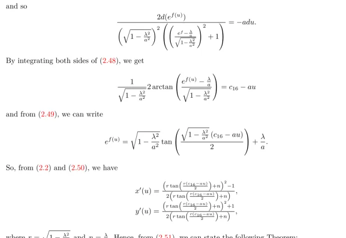
and so 2d(ef (u)₎ (√ 1−λ2 a2 )2  ( ef₋λ a √ 1−λ2 a2 )2 + 1   =−adu. (2.48)

By integrating both sides of (2.48), we get 1 √ 1−λ2 a2 2 arctan  e_√f (u)−λa 1−λ2 a2   = c16− au (2.49)

and from (2.49), we can write

ef (u) = √ 1−λ 2 a2 tan   √ 1−λ_a22(c16− au) 2   + λ a. (2.50)

So, from (2.2) and (2.50), we have

x′(u) = ( r tan(r(c16−au)₂ )+n)2₋₁ 2(r tan(r(c16−au)₂ )+n) , y′(u) = ( r tan(r(c16−au)₂ )+n)2+1 2 ( r tan ( r(c16−au) 2 ) +n ) , (2.51) where r =√1−λ_a22 and n = λ

a. Hence, from (2.51), we can state the following Theorem:

Theorem 2.7 The spacelike curve α(u) with constant weighted curvature κφ= λ in Lorentz-Minkowski plane

with density eax _{for −1 <} λ

a < 1 is

α(u) =  

nc16+2 lncos(r(c16−au)2 )+2 ln(n cos(r(c16−au)2 )+r sin(r(c16−au)2 ))

2a + c17,

n(2au−c16)+2 lncos(r(c16−au)2 )−2 ln (n cos(r(c16−au)2 )+r sin(r(c16−au)2 ))

2a + c18



 , (2.52)

where tan(r(c16−au)

2 ) >− n r, r = √ 1−λ_a22, n = λ a and ci∈ R, i = 16, 17, 18.

Figure 2 (e) shows this curve for λ = 1, a =−5, −4, −3, −2, 2, 3, 4, 5, c16= 1 and c17= c18= 0 .

So, taking λ = 0 in (2.52), we have:

Corollary 2.8 The spacelike curve α(u) with vanishing weighted curvature κφ in Lorentz-Minkowski plane

with density eax _{is given by}

α(u) =  ln  sin(c16−au) 2   a + c17, lncot(c16−au 2 ) a + c18   , (2.53)

where tan(r(c16−au)

2 ) >− n

r and ci∈ R, i = 16, 17, 18.

2.3. The case of ” a = 0, b̸= 0”

In this case, the equation (2.3) can be rewritten as

f′(u)− b sinh(f(u)) = λ. (2.54)

So, from (2.54), we have

2f′(u)ef (u)= b [( ef+λ b )2 − ( λ2 b2 + 1 )] . (2.55)

Now, we can find the spacelike curves by solving the equation (2.55) according to cases of constant λ.

2.3.1. Solving equation (2.55) for λ = 0 :

Firstly, let us assume that f′(u) = 0 . Then, from equation (2.55) we have

ef (u) = 1. (2.56)

So, from (2.2) and (2.56), we get

x(u) = d1,

y(u) = u + d2, d1, d2∈ R. (2.57)

Now, let us take f′(u)̸= 0. From equation (2.55),

2f′(u)ef (u)= b[(ef (u) )2 − 1 ] (2.58) and so, ( 1 ef (u)− 1− 1 ef (u)_{+ 1} )

d(ef (u)) = bdu. (2.59)

By integrating both sides of (2.59), we get 

e_ef (u)f (u)− 1_{+ 1}

 = ebu+d3_{. (2.60)}

Thus, we can write

ef (u)= 1 + e bu+d3 1− ebu+d3 (2.61) or ef (u)= 1− e bu+d3 1 + ebu+d3. (2.62)

Hence, using (2.61) and (2.62) in (2.2), we reach that

x′(u) = 1+ebu+d3 1−ebu+d3− 1−ebu+d3 1+ebu+d3 2 , y′(u) = 1+ebu+d3 1−ebu+d3+ 1−ebu+d3 1+ebu+d3 2 (2.63)

and x′(u) = 1−ebu+d3 1+ebu+d3− 1+ebu+d3 1−ebu+d3 2 , y′(u) = 1−ebu+d3 1+ebu+d3+ 1+ebu+d3 1−ebu+d3 2 , (2.64)

respectively. Thus, from (2.3.1), (2.63) and (2.64) we can give the following Theorem:

Theorem 2.9 The spacelike curves with vanishing weighted curvature κφ in Lorentz-Minkowski plane with

density eby _are

i) the straight line of

α(u) = (d1, u + d2), (2.65)

whose slope of lines is ∞, i.e. the lines are vertical and di∈ R, i = 1, 2;

ii) α(u) = ( ln(e−bu+ed3 e−bu−ed3) b + d4,−( ln(e−2bu− e2d3₎ b + u) + d5 ) , (2.66) where bu + d3< 0 and di∈ R, i = 3, 4, 5 or iii) α(u) = ( ln(e−bu_−ed3 e−bu+ed3) b + d6,−( ln(e−2bu− e2d3₎ b + u) + d7 ) , (2.67) where bu + d3< 0 and di∈ R, i = 3, 6, 7.

Figure 3 (a) and (b) show the curves (2.66) and (2.67), respectively, for b =−1, −2, −3, −4, −5, d3=−1 and d4= d5= d6= d7= 0 .

2.3.2. Solving equation (2.55) for λ̸= 0:

Firstly, let’s assume that f′(u) = 0 . From equation (2.55), we get

b [( ef (u)+λ b )2 − ( λ2 b2 + 1 )] = 0 (2.68) and so, ef (u) = √ (λ b) 2_{+ 1}−λ b. (2.69)

Thus, from (2.2) and (2.69), we have

x′(u) = √ (λ b)2+1−λb−√ 1 ( λ_b)2 +1− λ_b 2 , y′(u) = √ (λ b)2+1− λ b+ 1 √ ( λ_b)2 +1− λ_b 2 . (2.70)

Figure 3. The spacelike curves with constant weighted curvature in Lorentz-Minkowski plane with density eby _for different values of constant b .

Now, if f′(u)̸= 0, then the equation (2.55) can be rewritten as 2f′(u)ef (u) ( ef (u)₊λ b − √ λ2 b2 + 1 ) ( ef (u)₊λ b + √ λ2 b2 + 1 ) = b (2.71) and so,   1 ef (u)₊λ b − √ λ2 b2 + 1 − 1 ef (u)₊λ b + √ λ2 b2 + 1   d(e_√ f (u)) λ2 b2 + 1 = bdu. (2.72)

By integrating both sides of (2.72), we get    ef (u)₊λ b − √ λ2 b2 + 1 ef (u)₊λ b + √ λ2 b2 + 1   = eb √ λ2 b2+1u+d10. (2.73) Thus ef (u)₊λ b − √ λ2 b2 + 1 ef (u)₊λ b + √ λ2 b2 + 1 = eb √ λ2 b2+1u+d10 ⇒ ef (u)₌( λ b + √ λ2 b2 + 1)e b √ λ2 b2+1u+d10+ √ λ2 b2 + 1− λ b 1− eb √ λ2 b2+1u+d10 (2.74)

or ef (u)+λ_b − √ λ2 b2 + 1 ef (u)₊λ b + √ λ2 b2 + 1 =−eb √ λ2 b2+1u+d10 ⇒ ef (u) ₌ √ λ2 b2 + 1− λ b − ( λ b + √ λ2 b2 + 1)e b √ λ2 b2+1u+d10 1 + eb √ λ2 b2+1u+d10 . (2.75)

So, using (2.74) and (2.75) in (2.2), we have

x′(u) = ( (t+s)ebsu+d10 +s−t 1−ebsu+d10 )2 −1 2 ( (t+s)ebsu+d10 +s−t 1−ebsu+d10 ) , y′(u) = ( (t+s)ebsu+d10 +s−t 1−ebsu+d10 )2 +1 2 ( (t+s)ebsu+d10 +s−t 1−ebsu+d10 ) (2.76) and x′(u) = ( s−t−(t+s)ebsu+d10 1+ebsu+d10 )2 −1 2 ( s−t−(t+s)ebsu+d10 1+ebsu+d10 ) , y′(u) = ( s−t−(t+s)ebsu+d10 1+ebsu+d10 )2 +1 2 ( s−t−(t+s)ebsu+d10 1+ebsu+d10 ) , (2.77) respectively, where s = √ λ2 b2 + 1 and t = λ b.

So, from (2.70), (2.76) and (2.77), we have

Theorem 2.10 The spacelike curves with non-zero constant weighted curvature κφ= λ in Lorentz-Minkowski

plane with density eby _are

i) The straight line of

α(u) = ( ( s− t − _s−t1 2 ) u + d8, ( s− t +_s−t1 2 ) u + d9), (2.78)

whose slope of lines is (s_(s−t)−t)22+1₋₁ and di∈ R, i = 8, 9;

ii) α(u) =   u 2 ( 1 t+s− t − s ) −1 b (

ln(e−bsu− ed10)− ln(ed10_{(t + s) + (s}− t)e−bsu_{)) + d}

11, −u 2 ( 1 t+s + t + s ) −1 b (

ln(e−bsu− ed10)_{+ ln(e}d10_{(t + s) + (s}− t)e−bsu_{)) + d} 12



 , (2.79)

iii) α(u) =   u 2 ( 1 t+s− t − s ) −1 b (

lne−bsu− ed10 − ln_(s− t)e−bsu− ed10(t + s))_{+ d} 13, −u 2 ( 1 t+s+ t + s ) −1 b (

lne−bsu+ ed10_{+ ln}(s− t)e−bsu− ed10(t + s))_{+ d} 14



 , (2.80)

where ebsu+d10 _< s−t

s+t and di∈ R, i = 10, 13, 14. Here we take s =

√

λ2

b2 + 1 and t = λ b.

Figure 3 (c) and (d) show the curves (2.79) and (2.80), respectively, for λ = 1, b =−4, −3, −2, −1, 1, 2, 3, 4,

d10=−10 and d11= d12= d13= d14= 0 .

3. Timelike curves with constant weighted curvature in Lorentz-Minkowski plane with density

eax+by

In this section, we obtain the weighted curvature κφ of a timelike curve β in Lorentz-Minkowski plane with

density eax+by _{and investigate the timelike curves with constant weighted curvature for some cases of not all}

zero constants a and b with the same procedure in the previous section.

The weighted curvature κφ(u) of a timelike curve β(u) = (x(u), y(u)) with arc-length paremeter in

Lorentz-Minkowski plane with density eax+by _{is obtained as}

κφ= x′(u)y′′(u)− x′′(u)y′(u) + ay′(u)− bx′(u). (3.1)

Since β(u) = (x(u), y(u)) is a timelike curve with arc-length papameter, we can take x′(u) = cosh(f (u)),

y′(u) = sinh(f (u)). (3.2)

So, from (3.1) and (3.2), the constant weighted curvature κφ can be written as

κφ= f′(u) + a sinh(f (u))− b cosh(f(u)) = λ, (3.3)

where λ∈ R.

Now, let us obtain the timelike curves with constant weighted curvature λ according to some cases of constants a and b.

3.1. The case of ” a = b”

In this case, the equation (3.3) can be rewritten as

f′(u) + a sinh(f (u))− a cosh(f(u)) = λ. (3.4)

Using the definition of the hyperbolic functions in (3.4), we have

f′(u)ef (u)= a + λef (u). (3.5)

Now, we can find the timelike curves by solving the equation (3.5) according to cases of constant λ.

Theorem 3.1 The timelike curve β(u) with vanishing weighted curvature in Lorentz-Minkowski plane with density ea(x+y) _is β(u) = ( au(au + 2l1) + 2 ln(au + l1) 4a + l2, au(au + 2l1)− 2 ln(au + l1) 4a + l3 ) , (3.6) where au + l1> 0 and li∈ R, i = 1, 2, 3.

Figure 4 (a) shows this curve for a =−5, −4, −3, −2, −1, 1, 2, 3, 4, 5, l1= 6 and l2= l3= 0 .

Figure 4. The timelike curves with constant weighted curvature in Lorentz-Minkowski plane with density ea(x+y) _for different values of constant a .

Theorem 3.2 The timelike curves with non-zero constant weighted curvature κφ = λ in Lorentz-Minkowski

plane with density ea(x+y) _are

i) the straight line of

β(u) = ( −a2_{− λ}2 2aλ u + l4, λ2_{− a}2 2aλ u + l5 ) , (3.7) whose slope is a2_−λ2

a2_+λ2. In the case of a =−λ, the slope of lines is 0, i.e. the lines are horizontal, where

a λ < 0 and li∈ R, i = 4, 5; ii) β(u) = ( eλu+l6− au 2λ + lnλel6− ae−λu 2a + l7, eλu+l6− au 2λ − lnλel6− ae−λu 2a + l8 ) , (3.8) where ae−λu λ < e l6 and l i∈ R, i = 6, 7, 8 or iii) β(u) = ( lnae−λu+ λel6 2a − eλu+l6_{+ au} 2λ + l9,− lnae−λu+ λel6 2a − eλu+l6_{+ au} 2λ + l10 ) , (3.9)

where −el6 _> ae−λu

Figure 4 (b) shows the curve (3.8) for λ = 1, a =−5, −4, −3, −2, −1, 1, 2, 3, 4, 5, l6= 10 and l7= l8= 0 and

Figure 4 (c) shows the curve (3.9) for λ = 10, a = 1, 2, 3, 4, 5, l6=−1 and l9= l10= 0.

3.2. The case of ” a = 0, b̸= 0”

In this case, the equation (3.3) can be rewritten as

f′(u)− b cosh(f(u)) = λ. (3.10) From (3.10), we have 2f′(u)ef (u) = b [( ef (u)+λ b )2 + 1−λ 2 b2 ] . (3.11)

Now, we can obtain the timelike curves by solving the equation (3.11) according to cases of constant λ. So, we have the following Theorems which can be obtained with the same procedure in Subsection 2.2.

Theorem 3.3 The timelike curves β(u) with constant weighted curvature κφ= λ in Lorentz-Minkowski plane

with density eby _{for λ =−b are}

i) the straight line of

β(u) = (u + h1, h2) (3.12)

whose slope of lines is 0, i.e. the lines are horizontal and hi∈ R, i = 1, 2 or

ii) β(u) =  bu + ln ( bu+h3−2 bu+h3 ) b + h4,− ln((bu + h3)(bu + h3− 2)) b + h5   , (3.13) where bu + h3∈ R − [0, 2] and hi∈ R, i = 3, 4, 5.

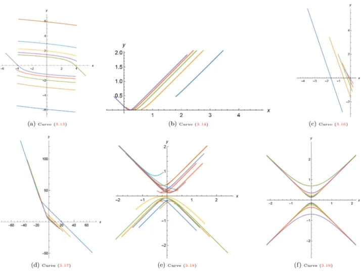
Figure 5 (a) shows the curve (3.13) for λ =−b = −5, −4, −3, −2, −1, 1, 2, 3, 4, 5, h3= 20 and h4= h5= 0.

Theorem 3.4 The timelike curve β(u) with constant weighted curvature κφ= λ in Lorentz-Minkowski plane

with density eby _{for λ = b is}

β(u) =  −bu + ln   h6+bu 2+h6+bu   b + h7,− ln|(h6+ bu)(2 + h6+ bu)| b + h8   , (3.14) where bu + h6∈ (−2, 0) and hi∈ R, i = 6, 7, 8.

Figure 5 (b) shows this curve for λ = b = 1, 2, 3, 4, 5 and h6= h7= h8= 0 .

Theorem 3.5 The timelike curves with constant weighted curvature κφ= λ in Lorentz-Minkowski plane with

density eby _for λ

Figure 5. The timelike curves with constant weighted curvature in Lorentz-Minkowski plane with density eby _for different values of constant b .

i) the straight line of

β(u) = (( −t ± p + 1 −t±p 2 ) u + h9, ( −t ± p − 1 −t±p 2 ) u + h10 ) , (3.15) whose slope is (−t±p)2−1 (−t±p)2₊₁ and hi ∈ R, i = 9, 10; ii) β(u) =    −u2 ( t + p +_t+p1 ) − (ln( e−bpu−eh11 (p−t)e−bpu+(p+t)eh11) b ) + h12, −u 2 ( t + p−_t+p1 )

− (ln((e−bpu_−eh11_)((p−t)e−bpu_+(p+t)eh11₎₎

b ) + h13

 

 , (3.16)

where (1− eh11+bpu_{) and ((p + t)e}bpu+h11_{+ p}− t) have same signs and h

iii) β(u) =   −u2 ( t + p +_t+p1 )

− (ln(e−bpu+eh11)−ln|(pb−t)e−bpu−(p+t)eh11|) + h14, −u

2

(

t + p−_t+p1 )

− (ln(e−bpu+eh11)+ln|(pb−t)e−bpu−(p+t)eh11|) + h15



 , (3.17)

where hi∈ R, i = 11, 14, 15. Here, we take p =

√

λ2

b2 − 1, t =

λ b.

Figure 5 (c) shows the curve (3.16) for λ = 6, b = −1, −2, −3, −4, −5, h11 =−61 and h12 = h13 = 0 and

Figure 5 (d) shows the curve (3.17) for λ = 11, b =−1, −2, −3, −4, −5, h11= 10 and h14= h15= 0 .

Theorem 3.6 The timelike curve with constant weighted curvature κφ= λ in Lorentz-Minkowski plane with

density eby _for λ

b > 1 is given by (3.16).

Theorem 3.7 The timelike curve β(u) with constant weighted curvature κφ= λ in Lorentz-Minkowski plane

with density eby _{for −1 <} λ

b < 1 is

β(u) =   −

t(h16+2bu)+2 lncos(q(bu+h16)2 )−2 ln(t cos(q(bu+h16)2 )−q sin(q(bu+h16)2 ))

2b + h17, th16−2 lncos(q(bu+h16)2 )  −2 ln(t cos(q(bu+h16) 2 )−q sin(q(bu+h16)2 ))   2b + h18   , (3.18)

where tan(q(bu+h16)

2 ) > t q, q = √ 1−λ2 b2, t = λ b and hi∈ R, i = 16, 17, 18.

Figure 5 (e) shows this curve for λ = 1, b =−5, −4, −3, −2, 2, 3, 4, 5, h16= 1 and h17= h18= 0 .

So, taking λ = 0 in (3.18), we have:

Corollary 3.8 The timelike curve β(u) with vanishing weighted curvature κφ in Lorentz-Minkowski plane with

density eby _{is given by} β(u) = ( lntan(bu+h16 2 ) b + h17, − ln1 2sin(bu + h16) b + h18 ) , (3.19)

where tan(q(bu+c16)

2 ) > t

q and hi∈ R, i = 16, 17, 18.

Figure 5 (f) shows this curve for b =−5, −4, −3, −2, −1, 1, 2, 3, 4, 5, h16= 1 and h17= h18= 0 .

3.3. The case of ” a̸= 0, b = 0”

In this case, the equation (3.3) can be rewritten as

f′(u) + a sinh(f (u)) = λ. (3.20)

So, from (3.20), we have

2f′(u)ef (u)=−a [( ef−λ a )2 − ( λ2 a2 + 1 )] . (3.21)

Now, we can find the timelike curves by solving the equation (3.21) according to cases of constant λ.

So, we have the following Theorems which can be obtained with the same procedure in Subsection 2.3.

Theorem 3.9 The timelike curves with vanishing weighted curvature κφ in Lorentz-Minkowski plane with

density eax _are

i) the straight line of

β(u) = (u + g1, g2), (3.22)

whose slope of lines is 0, i.e. the lines are horizontal and gi∈ R, i = 1, 2;

ii) β(u) = ( ln(e2au_{− e}2g3₎ a − u + g4, ln(eau_−eg3 eau_+eg3) a + g5 ) , (3.23) where au > g3 and gi∈ R, i = 3, 4, 5 or iii) β(u) = ( ln(e2au_{− e}2g3₎ a − u + g6, ln(eau+eg3 eau_−eg3) a + g7 ) , (3.24) where au > g3 and gi∈ R, i = 3, 6, 7.

Figure 6 (a) and (b) show the curves (3.23) and (3.24), respectively, for a = 1, 2, 3, 4, 5, g3 = −11 and g4= g5= g6= g7= 0 .

Figure 6. The timelike curves with constant weighted curvature in Lorentz-Minkowski plane with density eax _for different values of constant a

Theorem 3.10 The timelike curves with non-zero constant weighted curvature κφ= λ in Lorentz-Minkowski

plane with density eax _are

i) The straight line of

β(u) = ( ( v + n +_v+n1 2 ) u + g8, ( v + n−_v+n1 2 ) u + g9), (3.25)

whose slope of lines is (v+n)_(v+n)22−1₊₁ and gi∈ R, i = 8, 9; ii) β(u) =   u2 ( 1 n−v + n− v )

+1_a(ln(eavu_{− e}g10_{) + ln(e}g10_(n− v)2_{+ e}avu_{)) + g} 11, u 2 ( n− v −_n−v1 )

+1_a(ln(eavu− eg10₎− ln(eg10_(n− v)2_{+ e}avu_{)) + g} 12



 , (3.26)

where avu > g10 and gi∈ R, i = 10, 11, 12 or

iii) β(u) =   u2 ( 1 n−v + n− v ) +1 a(ln(e

avu_{+ e}g10_{) + ln(e}avu− eg10_(n− v)2_{)) + g} 13, u 2 ( n− v − 1 n−v ) +1 a(ln(e

avu_{+ e}g10₎− ln(eavu− eg10_(n− v)2_{)) + g} 14



 , (3.27)

where eavu−g10 _>n−v

n+v and gi∈ R, i = 10, 13, 14. Here we take v =

√

λ2

a2 + 1 and n = λ a.

Figure 6 (c) and (d) show the curves (3.26) and (3.27), respectively, for λ = 1, a = −5, −4, −3, −2, −1, 1, 2, 3, 4, 5, g10=−11 and g11= g12= g13= g14= 0 .

4. Conclusion and future work

In this study, we have obtained the weighted curvature κφof spacelike and timelike curves in Lorentz-Minkowski

plane with density eax+by _{and we have given the parametric expressions of the spacelike and timelike curves}

with constant weighted curvature for the cases of ” a = b”, ” a̸= 0, b = 0” and ”a = 0, b ̸= 0”. Also, we have construct some examples of obtained curves for different values of constants a and b.

We hope that, this study will bring a new viewpoint and break fresh ground to geometers who are dealing with the curves in a plane with density. And in the near future, spacelike and timelike curves in Lorentz-Minkowski plane with different densities can be investigated by geometers.

Acknowledgment

“This paper has been supported by Scientific Research Projects (BAP) unit of İnönü University (Malatya/TURKEY) with the Project number FDK-2018-1349.”

References

[1] Belarbi L, Belkhelfa M. Surfaces in R3_{with Density. i-manager’s Journal on Mathematics 2012; 1 (1): 34-48. doi:}

10.26634/jmat.1.1.1845

[2] Belarbi L, Belkhelfa M. Some Results in Riemannian Manifolds with Density. Analele Universitatii din Oradea. Fascicola Matematica 2015; Tom XXII, Issue No. 2: 81-86.

[3] Castro I, Castro-Infantes I, Castro-Infantes J. Curves in the Lorentz-Minkowski plane: elasticae, catenaries and grim-reapers. Open Mathematics 2018; 16: 747-766. doi: 10.1515/math-2018-0069

[4] Corwin I, Hoffman N, Hurder S, Sesum V, Xu Y. Differential geometry of manifolds with density. Rose-Hulman Undergraduate Mathematics Journal 2006; 7 (1): 1-15. Available at https://scholar.rose-hulman.edu/rhumj/vol7/iss1/2.

[5] Gromov M. Isoperimetry of waists and concentration of maps. Geometric and Functional Analysis 2003; 13: 178-215. [6] Hieu DT, Hoang NM. Ruled Minimal Surfaces in R3 _{with Density e}z_{. Pacific Journal of Mathematics 2009; 243(2):}

277-285.

[7] Hieu DT, Nam TL. The classification of constant weighted curvature curves in the plane with a log-linear density. Communications on Pure and Applied Analysis 2014; 13 (4): 1641-1652. doi: 10.3934/cpaa.2014.13.1641

[8] Kazan A, Karadağ HB. Weighted Minimal and Weighted Flat Surfaces of Revolution in Galilean 3-Space with Density. International Journal of Analysis and Applications 2018; 16 (3): 414-426. doi: 10.28924/2291-8639-16-2018-414

[9] López R. Differential Geometry of Curves and Surfaces in Lorentz-Minkowski space. International Electronic Journal of Geometry 2014; 7 (1): 44-107.

[10] López R. Minimal surfaces in Euclidean space with a log-linear density. arXiv:1410.2517v1 2014.

[11] Morgan F. Manifolds with Density. Notices of the American Mathematical Society 2005; 52 (8): 853-858. [12] Morgan F. Myers’ Theorem with Density. Kodai Mathematical Journal 2006; 29: 455-461.

[13] Morgan F. Manifolds with Density and Perelman’s Proof of the Poincare Conjecture. Mathematical Association of America 2009; 116 (2): 134-142.

[14] Nam TL. Some results on curves in the plane with log-linear density. Asian-European Journal of Mathematics 2017; 10 (2): 1-8. doi: 10.1142/S1793557117500851

[15] Yıldız ÖG, Hızal S, Akyiğit M. Type I+ _{Helicoidal Surfaces with Prescribed Weighted Mean or Gaussian Curvature}

in Minkowski Space with Density. Analele Universitatii ”Ovidius” Constanta-Seria Matematica 2018; 26 (3): 99-108. doi: 10.2478/auom-2018-0035

[16] Yoon DW. Weighted Minimal Translation Surfaces in Minkowski 3-space with Density. International Journal of Geometric Methods in Modern Physics 2017; 14 (12): 1-10. doi: 10.1142/S021988781750178X

[17] Yoon DW. Weighted Minimal Translation Surfaces in the Galilean Space with Density. Open Mathematics 2017; 15: 459-466. doi: 10.1515/math-2017-0043

[18] Yoon DW, Kim DS, Kim YH, Lee JW. Constructions of Helicoidal Surfaces in Euclidean Space with Density. Symmetry 2017; 9, 173: 1-9. doi: 10.3390/sym9090173

[19] Yoon DW, Yüzbaşı ZK. Weighted Minimal Affine Translation Surfaces in Euclidean Space with Density. Interna-tional Journal of Geometric Methods in Modern Physics 2018; 15 (11). doi: 10.1142/S0219887818501967