Balancing straight and U-Type assembly lines with stochastic process times

i

BALANCING STRAIGHT AND U-TYPE ASSEMBLY

LINES WITH STOCHASTIC PROCESS TIMES

A THESIS

SUBMITTED TO THE DEPARTMENT OF INDUSTRIAL ENGINEERING AND THE INSTITUTE OF ENGINEERING AND

SCIENCE OF BİLKENT UNIVERSITY

IN PARTIAL FULFILLMENT OF THE REQUIREMENTS FOR THE DEGREE OF

MASTER OF SCIENCE

By

Halil Şekerci

August, 2003

ii

I certify that I have read this thesis and that in my opinion it is fully adequate, in scope and in quality, as a thesis for the degree of Master of Science.

Prof. İhsan Sabuncuoğlu (Principal Advisor)

I certify that I have read this thesis and that in my opinion it is fully adequate, in scope and in quality, as a thesis for the degree of Master of Science.

Prof. Erdal Erel

I certify that I have read this thesis and that in my opinion it is fully adequate, in scope and in quality, as a thesis for the degree of Master of Science.

Asst. Prof. M. Murat Fadıloğlu

Approved for the Institute of Engineering and Science:

Prof. Mehmet Baray

iii

ABSTRACT

BALANCING STRAIGHT AND U-TYPE ASSEMBLY LINES

WITH STOCHASTIC PROCESS TIMES

Halil Şekerci

M.S. in Industrial Engineering

Advisor: Prof. İhsan Sabuncuoğlu

August,2003

In this thesis, we study the problem of assembly line balancing with stochastic task process times. The research considers both the well-known straight line balancing problem and U-line balancing problem where the line is paced, with no buffer inventories between stations. The objective is to minimize a two component cost function where the cost terms come from cost of manning the line and cost of finishing the incomplete units off the line. Cost is measured by an existing exact method for straight line balancing and a heuristic cost measurement method is developed for U-line balancing. The key idea in the core of this research is a task's marginal desirability for assignment at a given station. This idea is embedded in a beam search heuristic for solving both the straight line and U-line balancing problem. Extensive computational experiments and simulation experiments are made with well-known problems in the literature under the assumption of normally distributed task processing times. The quality of the solutions found by beam search for the straight-line balancing problem is compared to an existing method in literature. A simulation model of the assembly design is constructed and sample results from the U-line balancing problem are tested against the simulation results. The algorithm presented in this thesis improves the objective function by up to 24 percent.

iv

ÖZET

RASSAL İŞ ZAMANLI DÜZ VE U TİPİ MONTAJ HATLARININ

DENGELENMESİ

Halil Şekerci

Endüstri Mühendisliği, Yüksek Lisans

Tez Yöneticisi: Prof. Dr. İhsan Sabuncuoğlu

Ağustos 2003

Bu tezde Rassal İş Zamanlı Montaj Hatlarının Dengelenmesi problemi üzerinde çalışıldı. Araştırmamız hem iyi bilinen anuyumlu düz montaj hatlarını hem de anuyumlu U tipi montaj hatlarını istasyonlar arasında tampon envanterlerin yokluğunda incelemektedir. Amacımız işgücü maliyeti ve ürünü çevrimdışı montajlama maliyeti gibi iki bileşenli bir maliyet fonksiyonunu en azlamaktır. Maliyet düz hatlar için kesin, U tipi hatlar için ise sezgisel bir yöntemle hesaplanmaktadır. Bu araştırmanın temelinde yatan ana fikir bir işin verilen istasyondaki konuma atanması için marjinal istenilirliğinin belirlenmesidir. Bu fikir düz ve U tipi montaj hatlarının dengelenmesinde kullanılmak üzere bir ışın taraması sezgisel yönteminin içerisinde kullanılmıştır. İş zamanlarının normal dağılıma sahip olduğu varsayımı altında literatürdeki iyi bilinen problemler üzerinde kapsamlı hesapsal deneyler ve benzetim deneyleri gerçekleştirilmiştir. Işın taraması kullanılarak elde edilen sonuçların kalitesi düz montaj hatları için literatürdeki bir diğer yöntemin sonuçlarıyla karşılaştırılmıştır. Montaj hattının bir benzetim modeli kurularak U tipi montaj hatları için elde edilen sonuçlar benzetim modelinin sonuçlarıyla karşılaştırılmıştır. Bu tezde sunulan yöntem amaç fonksiyonunda % 24’lere varan iyileştirmeler sağlamıştır.

v

vi

ACKNOWLEDGEMENTS

I would like to express my deepest gratitude to Prof. İhsan Sabuncuoğlu and Prof. Erdal Erel who supervised me through all stages of this research. They are certainly not only supervisors of this thesis, but also a shareholder of it.

I am also indebted to Asst. Prof. M. Murat Fadıloğlu for his accepting to read and review this thesis.

My special thanks goes to İlktuğ Çağatay Kepek, for his invaluable friendship through my whole university life. He made me, never feel alone and was an indispensable part of our intelligent talks.

I would also like to thank to my friends, Aykut Özsoy, Onur Özkök, Hüseyin Özsert, Sabri Çelik, Müge Yayla, Savaş Çevik, Gökhan Metan, Ali Koç, Evren Emek, Sibel Alumur, Ünal Akmeşe for their friendship and morale support all the time. I am indebted to many others whose names are not on this page but whose love is in my heart for sure.

Finally, I owe so much to my family. Without their support, I could have never been the man I am.

vii

TABLE OF CONTENTS

CHAPTER 1 ... 1

INTRODUCTION... 1

1.1 A BRIEF HISTORY... 1

1.2 PRELIMINARIES OF THE ALBP ... 2

1.3 PRELIMINARIES OF U-LINE BALANCING... 5

1.4 VARIATIONS OF THE BALANCING PROBLEM... 8

1.5 IMPORTANCE OF THE PROBLEM... 9

1.6 THE SCOPE OF THIS STUDY... 10

1.7. ASSUMPTIONS OF THIS STUDY... 11

1.8 SUMMARY OF WORK DONE... 12

1.9 POTENTIAL CONTRIBUTIONS TO THE LITERATURE... 13

CHAPTER 2 ... 14

LITERATURE SURVEY... 14

2.1 SINGLE MODEL DETERMINISTIC ALBP ... 15

2.1.1 Optimum-Seeking Approaches ... 16

2.1.2 Heuristic Solution Approaches... 18

2.2 SINGLE MODEL STOCHASTIC ALBP ... 20

2.3 SINGLE MODEL DETERMINISTIC ULBP... 22

2.4 SINGLE MODEL STOCHASTIC U-LINE... 25

CHAPTER 3 ... 27

PROPOSED METHOD... 27

3.1 STRUCTURE OF BEAM SEARCH... 27

3.2 BEAM SEARCH BASED ALGORITHM FOR OUR PROBLEM... 29

3.2.1 Search tree representation ... 30

3.2.2 Search methodology ... 31

3.2.3 The search procedure... 31

viii

3.3.1 Heuristic for completing partial designs... 33

3.3.2 Procedure for evaluating designs... 35

3.4 THE EVALUATION MECHANISM FOR U-LINE... 40

3.4.1 Heuristic for completing partial designs... 40

3.4.2 Heuristic for evaluating designs... 41

CHAPTER 4 ... 44

EXPERIMENTAL SETTING ... 44

CHAPTER 5 ... 48

COMPUTATIONAL RESULTS ... 48

5.1 COMPUTATIONAL RESULTS FOR SLBP ... 48

5.2 COMPUTATIONAL RESULTS FOR ULBP... 57

5.3 ANALYSIS OF RESULTS FOR ULBP AND SLBP ... 66

CHAPTER 6 ... 73

ix

LIST OF TABLES

TABLE 2.1: SUMMARY OF LITERATURE ON STOCHASTIC PACED STRAIGHT LINE

BALANCING PROBLEM... 24

TABLE 2.2: SUMMARY OF WORK DONE ON PACED U-LINE BALANCING PROBLEM.. 26

TABLE 3.1: SUPPORTING DATA FOR THE EXAMPLE PROBLEM... 38

TABLE 3.2: ALL INCOMPLETION COMBINATIONS AND THEIR RESPECTIVE PROBABILITIES... 39

TABLE 3.3: TASK MEANS:(TI FOR THE ITH TASK)... 42

TABLE 3.4: TASK VARIANCES:(σ2I FOR THE ITH TASK) ... 42

TABLE 5.1: RESULTS FOR JACKSON'S 11 TASK PROBLEM... 51

TABLE 5.2 RESULTS FOR MITCHELL'S 21 TASK PROBLEM... 52

TABLE 5.3RESULTS FOR SAWYER'S 30 TASK PROBLEM... 53

TABLE 5.4: RESULTS FOR KILBRID'S 45 TASK PROBLEM... 54

TABLE 5.5: RESULTS FOR WARNECKE'S 58 TASK PROBLEM... 55

TABLE 5.6: RESULTS FOR TONGE'S 70 TASK PROBLEM... 56

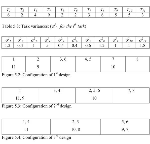
TABLE 5.7. TASK MEANS:(TI FOR THE ITH TASK)... 58

TABLE 5.8: TASK VARIANCES:(σ2I FOR THE ITH TASK) ... 58

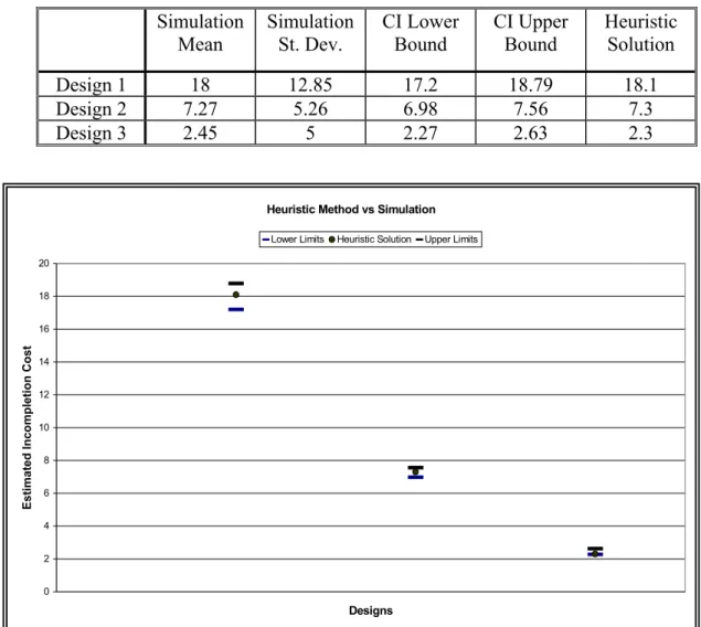
TABLE 5.9: COMPARISON OF SIMULATION RESULTS AND PROPOSED HEURISTIC RESULTS... 59

TABLE 5.10: RESULTS FOR JACKSON'S 11 TASK PROBLEM... 62

TABLE 5.11: RESULTS FOR MITCHELL'S 21 TASK PROBLEM... 62

TABLE 5.12: RESULTS FOR SAWYER'S 30 TASK PROBLEM... 63

TABLE 5.13: RESULTS FOR KILBRIDGE'S 45 TASK PROBLEM... 63

TABLE 5.14: RESULTS FOR WARNECKE'S 58 TASK PROBLEM... 64

TABLE 5.15: RESULTS FOR TONGE'S 70 TASK PROBLEM... 64

TABLE 5.16: COST COMPARISON OF DIFFERENT LINE CONFIGURATIONS... 65

TABLE 5.17: ANALYSIS OF VARIANCE FOR EFFECT OF LINE CONFIGURATION ON LINE COST... 68

TABLE 5.18: ANALYSIS OF VARIANCE FOR EFFECT OF LINE CONFIGURATION ON LINE COST... 68

TABLE 5.19: ANALYSIS OF VARIANCE FOR EFFECT OF LINE CONFIGURATION ON LINE COST... 69

x

TABLE 5.20: ANALYSIS OF VARIANCE FOR EFFECT OF LINE CONFIGURATION ON LINE COST... 69 TABLE 5.21: ANALYSIS OF VARIANCE FOR EFFECT OF VARIABILITY ON STRAIGHT

LINE COST... 70 TABLE 5.22: ANALYSIS OF VARIANCE FOR EFFECT OF VARIABILITY ON U-LINE COST

... 70 TABLE 5.23: FACTORS AND THEIR LEVELS... 71 TABLE 5.24: ANALYSIS OF VARIANCE OF LINE OPERATING COST FOR THREE

xi

LIST OF FIGURES

FIGURE 1.1: A PRECEDENCE RELATIONSHIP DIAGRAM. ... 3

FIGURE 1.2: STRAIGHT AND U-LINE CONFIGURATIONS. ... 6

FIGURE 1.3: SINGLE MODEL STOCHASTIC LINE BALANCING COSTS... 10

FIGURE 2.1: CLASSIFICATION OF ALBP AND RELATED SOLUTION PROCEDURES.... 15

FIGURE 3.1: REPRESENTATION OF A BEAM SEARCH TREE... 28

FIGURE 3.2: A PRECEDENCE DIAGRAM AND CORRESPONDING SEARCH TREE... 30

FIGURE 3.3: FLOW CHART OF LINE BALANCING ALGORITHM... 36

FIGURE 3.4: PRECEDENCE DIAGRAM OF THE EXAMPLE PROBLEM... 38

FIGURE 3.5: PRECEDENCE DIAGRAM OF THE EXAMPLE PROBLEM... 42

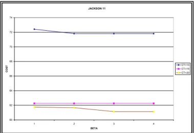
FIGURE 4.1:THE IMPACT OF BEAM WIDTH FOR JACKSON'S 11 TASK PROBLEM. ... 47

FIGURE 4.2:THE IMPACT OF BEAM WIDTH FOR SAWYER'S 30 TASK PROBLEM... 47

FIGURE 4.3:THE IMPACT OF BEAM WIDTH FOR TONGE'S 70 TASK PROBLEM. ... 47

FIGURE 5.1: PRECEDENCE DIAGRAM FOR THE TEST PROBLEMS. ... 58

FIGURE 5.2: CONFIGURATION OF 1ST DESIGN... 58

FIGURE 5.3: CONFIGURATION OF 2ND DESIGN... 58

FIGURE 5.4: CONFIGURATION OF 3RD DESIGN... 58

FIGURE 5.5: CONFIDENCE INTERVAL AND HEURISTIC SOLUTION FOR TEST PROBLEMS. ... 59

1

Chapter 1

Introduction

1.1 A brief history

Development of assembly lines is perhaps one of the most important triumphs of the twentieth century. The advent of assembly line in production systems, triggered mass production and made many products available to the benefit of mankind at reasonable prices. Although the first assembly line is credited to Henry Ford who developed such a line in 1913 and used it to produce Ford automobiles, the analysis and analytical statement of the assembly line balancing problem dates back only to 1955 (Salveson 1955). Jackson (1956), Bowman (1960), Supnik and Solinger (1960), White and Hu (1961) later followed his work. Extensive research on the assembly line balancing problem (ALBP) has accumulated since then, but the structure of the problem consistently defied the development of exact algorithms. Several survey papers review the work published on the subject: Kilbridge and Wester (1962), Ingall (1965), Mastor (1970), Buxey et al. (1973), Johnson (1981), Baybars (1986b), Yano and Bolat (1989), Erel and Sarin (1998), Amen (2000). In this section the concept of assembly line and the problem of assembly line balancing is introduced on straight shaped and U-shaped line configurations.

2

1.2 Preliminaries of the ALBP

An assembly line is a production sequence of stations connected together by a material handling system, where parts are assembled together at stations to form an end product. In this system there are work elements to be performed each of which is called a task. A task is the smallest indivisible work element in the assembly process.

Several tasks are performed at a physical location by a single worker and other tasks are similarly performed by other workers at different stations. A station is a location along the line at which tasks are performed by completing the assembly operations.

Task performance time, ti is the duration of task i, and cycle time C is the

amount of time available at each station. Equivalently cycle time is defined as the amount of time elapsed between two successive units entering or leaving the assembly line. Accordingly, station time Sj is defined as the sum of task times of

the tasks assigned to station j on the line.

After the line begins to give the first product, a partially assembled product remains at each station during each cycle, while the set of tasks assigned to this station is performed on it. The material handling system then moves all partially assembled parts forward to next station and a new cycle begins. Thus all the units at every station advance to their next station in sequence at the same time. This time point is the end of cycle time. Thus, if tasks are completed on a unit before the cycle time ends, the unit waits idle until the end of cycle time. Because of this synchronization in movement, these type of assembly lines are sometimes called as "synchronous lines".

Since there must exist at least one station and at least one task at each station, cycle time is bounded by the following relation :

Tasks are not completed arbitrarily, rather there exists a precedence relationship between the tasks, dictating the completion of some tasks before

1,.., 1,.., ₁

max _i max _j N _i

3 others can be started. A precedence diagram depicts the ordering, in which tasks must be performed to achieve a successful assembly of the product. This precedence diagram is either represented by a network of tasks or by an upper triangular NxN matrix, where N is the number of tasks in the assembly process. In the network representation, an arc originating from task i and ending at task j represents that task i must be completed before task j can be begun. In the matrix representation the entry [i,j] is 1 if task j follows task i in the precedence diagram, otherwise it is zero. Network representation is illustrated in Figure 1.1.

Figure 1.1: A precedence relationship diagram.

The assembly line balancing problem (ALBP) can be stated as assigning tasks to an ordered sequence of stations such that the precedence relations among the tasks are satisfied and some performance measure is optimized. The most commonly used objectives can be classified into two categories. In the first category one desires to minimize the number of stations given the cycle time. In this category we minimize number of stations subject to the following constraints.

(1) All tasks must be performed

(2) The work content in any station is less than or equal to the cycle time C. (3) Precedence relations are not violated.

Notice that such an objective is equivalent to minimizing the total idle time, since

where K is the number of stations in the design, under consideration.

Thus, when idle time is minimized K is also minimized. The reduction is due to the fact that is constant and C is given. This category is known as the Type I problem. 1 * N _i i Idle time K C t = = −

∑

∑

4 In the other category the objective is to minimize cycle time given the number of stations. This category is known as Type II problem. In both categories minimization is subject to precedence constraints.

A general integer programming formulation to the Type I problem is given as follows:

1 0 ij

if task i is assigned to station j i I and j J x othervise ∀ ∈ ∀ ∈   =    

N represents the number of tasks in the problem, K represents the total number of stations in the design (K≤ N), and F(i) represents the set of tasks that are immediate precedence followers of task i.

In this formulation the objective function (1) minimizes the number of stations opened by minimizing the station number assigned to the terminating task. Constraint (2) is known as assignment constraint and states that each task is assigned exactly to one station. Constraint (3) is the precedence constraint and states that all predecessors of task i must previously be assigned in order to assign it to a station. Constraint (4) is the cycle time constraint and states that station times can’t exceed the cycle time. Constraint (5) is the nondivisibility constraint of tasks.

Although the problem is easy to formulate, it has enormously large number of feasible solutions. Ignoring the precedence constraints, there are N! different orderings possible. Precedence relations decrease the number of feasible solutions

{ }

∑

∑

∑

∑

∑

5 drastically, but nevertheless the solution space is still too large to enumerate. Both Type I and Type II assembly line balancing problems are known to be NP-hard because the partition problem is known to be NP-hard (Papadimitriou, 1982). There is a vast number of heuristics and exact procedures in the literature to solve this problem.

There are also some other objectives offered in the literature other than the ones mentioned above. Smoothness index is a measure of how uniformly the workload is distributed among stations and is given by

Here sj represents the total mean task duration at station j. Smax is the maximum of

these statistics among all stations.

A measure of efficiency is balance delay, which is the ratio of the total idle time and the total time spent by a product moving from beginning to the end of line. It is given by:

Balance delay measures the idle percent of time that the unit spends on line.

1.3 Preliminaries of U-line balancing

The key difference between the traditional (straight) assembly line balancing problem and the U-line balancing problem is the following: In the straight line balancing problem, units to be processed enter the line from the head of the line and proceed their way to next station as operations are completed on them. Finally completed units leave the line from the end of the line. Hence the units flow in one direction which is from the head of the line to its rear. However, in a U-line units enter the line and traverse all stations from first to last and return all the way back from last station to first. In U-line configuration a station has at any time two units, one moving in forward direction and the other in backward direction. Workers at any station first complete the necessary tasks on the forward moving

∑

∑

6 unit, then they may turn to finish tasks on backward moving unit. Hence the completed parts leave the line from the first station. Straight line and U-line configurations are illustrated in Figure 1.2.

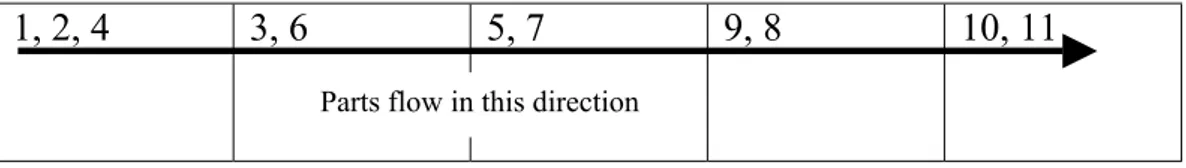
1, 2, 4 3, 6 5, 7 9, 8 10, 11

A straight line configuration with 11 tasks assigned to stations.

1, 2 11 4, 6 9 3 10 5 7, 8

A U-line configuration with 11 tasks assigned to stations.

Figure 1.2: Straight and U-line configurations.

Feasible U-line designs can be generated quite easily; the procedure is very similar to the straight line balancing case but proceeds in both forward and backward directions. In the straight line balancing problem, tasks are selected from a set of available tasks for assignment in order to form a station. These tasks are the ones whose predecessors have already been assigned. In the U-line balancing problem, the set of tasks available for assignment is the union of the set of tasks whose predecessors and successors have already been assigned. In other words, tasks with all predecessors assigned, are available for assignment in forward direction. Similarly tasks with all successors assigned, are available for assignment in backward direction.

The need for U-line configuration in manufacturing environments arises from attempts to improve productivity and increase flexibility. Miltenburg and Wijngaard (1994) state the following advantages of U-line configurations:

Parts flow in this direction

7 1. Quick response to changes in environment (machine breakdowns, worker

absenteeism etc.)

2. Ease to adapt to changes in cycle time because of high potential to rebalance the line.

3. High level of participation between workers. 4. Flexibility for adding or removing workers

5. Require at most the same or fewer amount of stations than traditional lines.

U-lines also present some operational difficulties such as scheduling the movement of workers, dispatching jobs, etc. Moreover the line balancing problem of a U-line is much more complicated than the traditional line due to increased search space.

An integer programming formulation of U-line balancing problem due to Urban (1998) is as follows: min * min max 1 0 1 0 1 ij ij j Let

m theoretical minimum number of stations

m m m n

if task i of the original network is assigned to station j x

otherwise

if task i of the phantom network is assigned to station j y otherwise if stati z = ≤ ≤ ≤      =    =   = ; . ., 0

on j is utilized i e it is assigned tasks otherwise

  

8 When making assignments to stations two copies of the precedence network is used. One copy is considered for forward assignments and the other is used for backward assignments. The copy of the precedence network is also called as "phantom network". Forward assignments are made through the original network and backward assignments are made through the phantom network . In this formulation, P is the precedence set for which the element (r,s) indicates that task

r immediately precedes task s.

Constraint (1) ensures that every task is assigned to only one station either in original or phantom network. Constraint (2) and (3) ensures that sum of the task times assigned to each station does not exceed cycle time. Constraints (5) and (6) enforce the precedence relationships between tasks.

1.4 Variations of the balancing problem

The assembly line problem has not remained as originally formulated. In time there arose many varieties of the original problem such as mixed model line balancing, U-type line balancing, stochastic assembly line balancing, etc. One such category that deserves special attention is the one that assumes stochastic

(

)

(

)

(

)

(

)

(

)

(

)

∑

∑

∑

∑

∑

(

)

{ }

∑

9 task times rather than deterministic. In the stochastic assembly line balancing problem task times are assumed to be random variables. Thus with such a setting one cannot guarantee that all the tasks assigned at a station be completed within the cycle time. Therefore, stochastic line balancing problem considers incompletion to occur at stations and alternative policies to adapt in incompletion situations. Naturally, the objective function in the formulation of stochastic line balancing may be different from the ones in deterministic cases. Incompletion ratio (Suresh and Sahu 1994) and expected line operating cost (Kottas and Lau 1973, Silverman and Carter 1986) are two example objectives used in literature.

1.5 Importance of the problem

The motivation for this study stems from the fact that assembly lines play important roles in today's manufacturing technology and understanding their behavior under variability is crucial to a firm's competitiveness. In general, variability is known to be detrimental but at the same time impossible to eliminate totally. Production plants, although designed for perfect synchronization, unfortunately do not operate at full efficiency due to the considerable variability inherent to the system. Conway et al. (1987) mentions that even in today's manufacturing plants a value of 10 for the ratio of flow time to total processing time is hard to achieve. Since the laws governing the performance of manufacturing systems are not understood to the full extent, it would be useful to provide the manufacturer with some design principles and guidelines. Without doubt a generic line balancing heuristic that employs these principles will reveal valuable information to the manufacturer and this will in turn reduce the operating cost of the plant and increase its competitiveness.

The use of JIT production methods also initiated the need for multi-functional workers and proper design of machinery layout. This resulted in U-shaped production lines which improved visibility and communication between workers as well as reducing the number of stations. The number of stations required on a U-line is never more than that required on a traditional line. This property of U-lines indicates their importance on the cost of production. Although

10 U-lines are important, there is little amount of work available in the literature. Therefore we believe that this study will contribute to the U-line literature especially if we consider that the stochastic U-line balancing problem has only one published journal paper.

1.6 The scope of this study

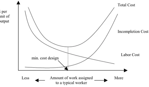
The problem investigated in this thesis is single model stochastic paced assembly line with straight and U-type configurations. Since task times are considered stochastic, operating costs incurred by balancing the line are affected by the cost of manning the line (labor cost), and the cost that arises from not completing the tasks as the unit moves down the line. These two cost terms are inversely related because the line operates at a constant output rate and amount of work to complete each unit on the line remains constant. The more work assigned to a worker reduces the number of workers needed but however it also increases the probability that the allocated work will not be completed within the given cycle time. Thus, a balance is to be established between these two cost terms given the cycle time. Figure 1.3 illustrates the situation.

Figure 1.3: Single model stochastic line balancing costs. (From Kottas and Lau (1973)) Total Cost Incompletion Cost Labor Cost $ per unit of output

Less Amount of work assigned More

to a typical worker min. cost design

11 Kottas and Lau (1973) report that industrial practice is to give some time allowance to the workers so that a variation in task time can be compensated without necessitating an incompletion. For this reason the industrial approach is to group the tasks into work assignments so that the sum of the expected task times does not exceed some specified percentage of the cycle time. However, as Kottas and Lau (1973) point out, this approach leaves two critical questions unanswered: Up to what percent of the cycle time should work stations be filled, and should this percentage be the same for all stations?

1.7. Assumptions of this study

The following assumptions are made about the assembly line considered in this research. These assumptions are the same as the ones adopted by Kottas and Lau (1973).

1. The cycle time and precedence relationships are the only restrictions on task assignments.

2. Each worker is paid the same wage regardless of the assignment 3. A task can only be begun if all its predecessors are completed.

4. The time to complete any task i is normally distributed with mean µi and

standard deviation σi and further, the performance time of any task is

independent of other task times and ordering of tasks within a station. 5. Whenever a task is not finished, the unit goes down the line with as many

of the remaining tasks being completed as possible. All unfinished tasks are completed off-line. The cost to complete task i offline is not a function of what fraction of the task i was completed on the line.

The first three assumptions are very common in the assembly line balancing literature (Kottas and Lau (1973), Silverman and Carter (1986)). Normally distributed task times are widely used in the stochastic line balancing literature e.g. Mansoor (1968). Assumption 5 is just one of the possible line operating policies and closely approximates the situation often encountered in the assembly of automobiles and appliances (Kottas and Lau (1973)).

12 In this research stochastic straight line and stochastic U-type line balancing are studied. Therefore throughout the study tasks are assumed to come from a distribution function which is known in advance. The research concentrates on the ways to minimize the operating cost of these lines. To achieve this, line designs are generated and evaluated by heuristic methods.

1.8 Summary of work done

In this research a line balancing algorithm is developed for each of stochastic straight line balancing problem and stochastic U-line balancing problem. The objective in both problems is to minimize total cost of the line which comprises of labor cost and incompletion cost.

For the stochastic straight line balancing problem, Kottas and Lau's (1973) stochastic straight line balancing procedure and Kottas and Lau's (1976) straight line exact cost evaluation method is embedded in a beam search based algorithm to generate better designs in terms of cost than that of Kottas and Lau (1981). Several test problems are solved by the proposed method and the results are compared to that of Kottas and Lau's (1981) algorithm. Results indicate that the proposed heuristic can improve the solution found by Kottas and Lau's (1981) algorithm by up to 24 percent.

For the stochastic U-line balancing problem, Kottas and Lau's (1973) stochastic straight line balancing procedure is modified and streamlined. This procedure is embedded in a beam search based procedure together with a U-line cost evaluation heuristic which is developed by the author of this research. The efficiency of the heuristic cost estimation is compared with simulation results for several test problems. The results indicate for the test problems that the solution found by the heuristic is within 95% confidence interval of the simulation run results. The method developed for the U-line balancing problem is successful in that, it correctly estimates the cost of line with 95% confidence. Moreover, it is the first method in literature to estimate a cost based objective for the stochastic U-line balancing problem. Using the modified procedure together with beam search improves the quality of the solutions found.

13

1.9 Potential contributions to the literature

The contribution of this research to the existing literature is twofold. First the research presents a method for the stochastic U-type line balancing problem for which the first publication appeared only on February 2003. There is quite vast room for research on this field and U-type lines are becoming much more common as the JIT production philosophies get more popular. The second contribution is stemming from the heuristic method used in this research. Beam search, which is the main heuristic on which this research relies on, has never been used for single model assembly line balancing problem. In this respect this research is the first to use this search methodology for single model assembly line balancing problem. Beam search was previously being used in scheduling problems (Sabuncuoglu and Karabuk (1997), Sabuncuoglu and Bayiz (2000)) and for sequencing product types in mixed model assembly lines (Matanachai and Yano (2001)). Therefore this research presents a new usage area of beam search, namely the assembly line balancing. Moreover, the research gives valuable information on the basic principles of a good design over dominated designs.

14

Chapter 2

Literature Survey

ALBP's can be classified into four categories depending on whether task times are deterministic or stochastic and based on the variety of products assembled. These are: Single Model Deterministic (SMD), Single Model Stochastic (SMS), Multi/Mixed Model Deterministic (MMD) and Multi/Mixed Model Stochastic (MMS). The SMD version of the problem is the most common and the simplest version of the problem. In this version task times are known constants. The SMS version introduces stochastic task times, where the task times are not known in advance but rather the task time distribution is known. MMD version deals with the case when more than one type of item is produced on the same line and task times are known constants. Finally version MMS deals with producing more than one item on a single line where the task times are stochastic.

There are also other classification schemes based on movement of assembled parts along the line. In this scheme there are two distinct types, non-mechanical and moving belt lines. Operators on non-non-mechanical lines are unpaced since in these kind of lines a unit moves independent of other units when the process at the current station is complete. This type of transfer is called

asynchronous transfer. Moving belt lines are simply characterized by a conveyor

belt and are known as paced lines. In paced lines units at all stations move simultaneously. This type of transfer is called synchronous transfer.

In this survey single model deterministic and single model stochastic line balancing problems are covered. One classification of the ALBP and related solution procedures is presented in the survey paper of Erel and Sarin (1998). Their classification is introduced in Figure 2.1.

15 Figure 2.1: Classification of ALBP and related solution procedures

2.1 Single Model Deterministic ALBP

In this version of the problem, line is designed to produce only one model for which the task times are known with certainty. Thus, the problem is, given a finite set of tasks, a set of precedence constraints and a cycle time value, to assign tasks to an ordered sequence of stations such that the precedence relations are satisfied, total duration of tasks in any station does not exceed the cycle time and some performance measure is optimized. This problem is in the general class of sequencing and scheduling problems and is closely related to other problems in this class, such as single machine scheduling problem, bin packing and knapsack problem. Most of the studies on single model deterministic ALBP are about Type

Assembly Line Balancing Problems

Single Model Multi/mixed Model

Deterministic (SMD) Stochastic (SMS) Deterministic (MMD) Stochastic (MMS)

Exact

Algorithms Heuristics Heuristics Heuristics Algorithms Exact Heuristics

Single-pass

Procedures Procedures Multi-pass Backtracking Procedures Modified versions of SMD problem procedures Procedures developed solely for SMS problem

16 I problem. There are two approaches in the literature for this problem: optimum-seeking algorithms and heuristics.

2.1.1 Optimum-Seeking Approaches

The exact methods in Type I and Type II problems can be treated under two main categories. In the first category the commonly used formulations are 0-1 IP and solution methodologies are enumerative techniques like branch-and-bound. The first branch-and-bound algorithm was developed by Jackson (1956). Many other researchers followed his work with various optimum branching and optimum search strategies.

Johnson (1973) constructed a newest-node branch-and-bound algorithm and in 1981 he developed an improved version of his previous work (1973) by changing only the bounding mechanism.

Patterson and Albracht (1975) proposed a 0-1 IP formulation and the Fibonacci search procedure. In this method a sequence of 0-1 IP problems are examined to determine feasible solutions. They also used lower and upper bounds to reduce the number of variables.

Wee and Magazine (1981a) proposed a branch-and-bound algorithm that depends on two heuristics rather than the IP formulation. The first heuristic is called IUFFD (Immediate Update First-Fit Decreasing) and is a variation of the bin packing heuristic FFD (First-Fit Decreasing). The second heuristic is called IUBRPW (Immediate Update Backward Recursive Positional Weight) which is a reverse application of the well-known RPW (Ranked Positional Weight) technique.

Talbot and Patterson (1984) constructed a general IP algorithm and used network cuts and chains in order to expedite the backtracking in the problem. They have obtained optimal solutions for assembly lines up to 100 tasks in reasonable computational time.

Johnson (1988) proposed a method called FABLE (Fast Algorithm for Balancing Lines Effectively) which is a depth-first branch-and-bound algorithm. He used eight fathoming rules to shorten the search time.

17 Hoffman (1992) developed a depth-first branch-and-bound algorithm called EUREKA. This procedure searches all the branches by considering the "theoretical minimum slack time" fathoming rule. The method starts with theoretical minimum number of stations and if the cumulative sum of station slack times exceeds "theoretical minimum total slack time" then all emanating branches are fathomed. This method requires much computational effort.

Nourie and Venta (1991) proposed a method called OptPack which is a depth first search algorithm that checks solutions in lexicographic order until optimum is found.

Klein and Scholl (1996) proposed a branch-and-bound algorithm named as SALOME-2 for the Type II problem adapted from SALOME-1 (Scholl and Klein, 1994). This method uses a new enumeration technique, local lower bound method together with unidirectional and bi-directional search mechanisms.

Sprecher (1999) offered a competitive branch-and-bound algorithm for the Type I problem. His algorithm relies on a precedence tree guided enumeration scheme. He reformulates the ALBP as a resource-constrained project scheduling problem with single renewable resource whose availability varies with time and then uses branch-and-bound to solve the problem.

Amen (2000) proposed an exact method for cost oriented assembly line problem. He introduces an exact backtracking method in which the enumeration process is limited by modified and new bounding rules.

In the second category are the algorithms based on DP. The very first algorithm in this category was developed by Jackson (1956) although it was not formulated using the conventional DP terminology. A few years later a new DP algorithm was reported by Held and Karp (1962). Schrage and Baker (1978) proposed an efficient method for generating feasible sets. In their method, they define the feasible subsets of tasks and enumerate all of them with a labeling scheme. Their work was followed by Kao and Queyranne (1982). They defined a minimum cost function with the minimum number of stations needed for all tasks in their procedure. Computational experience indicates that as the size of the problem grows, the computational effort involved in DP algorithms increase enormously.

18

2.1.2 Heuristic Solution Approaches

The problem size sometimes makes it almost impossible to solve optimally. Therefore heuristic solution methodologies are developed to save from computational time at the cost of not guaranteeing the optimal solution. Heuristic procedures in single model deterministic ALBP are classified in three categories.

In the first category a single-pass decision rule is used. Such procedures prioritize some task based on a single attribute of each task using a list processing scheme.

The first and well-known was constructed by Helgeson and Birnie (1961) under the name Ranked Positional Weight Technique (RPWT). In this technique each task is given a weight equal to sum of its task time and task times of its followers. Then tasks are listed in decreasing weight and selection is made in that order as long as the cycle time and precedence constraints are not violated. If precedence constraints or cycle time constraint is violated, next task in the list is considered. If no further task can be assigned to the station, a new station is opened. Though its popularity, the method is shown to give very poor solutions by Ignall (1965) and by Mastor (1970) in their example problems.

There are other similar procedures which rank tasks according to some rule and selecting the highest rank task. Kilbridge and Wester (1961), proposed another heuristic that groups the tasks into columns in the precedence diagram and assigns them to stations by shifting their place in between groups.

Baybars (1986b) developed a heuristic that combines some tasks to reduce the size of the problem. Then he decomposes problem into smaller sub-problems to seek their solutions and finally he combines these solutions and decomposes tasks to reach the solution of the problem.

Wee and Magazine (1982) developed two heuristic procedures named RA (Rank-and-Assign) and GFF (Generalized First-Fit). These heuristics assign numerical scores to all tasks, ranks them in the descending order and selects them according to their rank and precedence relations.

19 The second category belongs to multiple-pass procedures. Arcus's (1966) technique called 'Computer Method of Sequencing Operations for Assembly Lines' (COMSOAL ) is well-known example in this category. The main idea in COMSOAL is random generation of a feasible sequence. The method determines the available tasks for assignment at every iteration and selects randomly among the available tasks to fill the remaining station time. The author also used variations of the method by biasing the selection of tasks available for assignment. Among the variants the combined method gave the best results.

Later, Schofield (1979), Nksau and Leung (1995) constructed similar procedures in which best design is selected among several generated.

Hackman, Magazine and Wee (1989) developed several heuristic fathoming rules for the branch-and-bound algorithm so that the size of the problem is reduced.

The third and the last category comprises procedures that try to improve a solution or a station assignment by some iterative backtracking methods. An example to this category is the two phase procedure of Moodie and Young (1965) where in the first phase a preliminary balance is obtained by selecting among the available tasks the one with the largest performance times. In the second phase of this algorithm tasks are transferred between stations so that idle time is evenly distributed among the stations. Chiang (1998) uses tabu search for the ALBP. In his paper he considers four different approaches that use either first or best improvement strategies with or without task aggregation. Goncalves and Almeida (2002) used a hybrid genetic algorithm for ALBP. Their chromosome representation of the problem is based on random keys. The assignment of tasks to stations are made by some heuristic rules. They also use a local search to improve the solution.

20

2.2 Single Model Stochastic ALBP

The Stochastic Assembly Line Balancing Problem can be stated as assigning a set of tasks to an ordered sequence of stations, where performance times of tasks are distributed according to a probability distribution, subject to precedence constraints such that some performance measure is optimized. Now that the task times are random variables, a task can be incomplete either because the task is not completed within cycle time C or it is the precedence follower of another incomplete task. Incompletions reduce the efficiency of the line because they decrease throughput. So an incompletion cost term is associated with SALBP and this term depends on how incompletions are handled. Incompletions can be completed off the line and in this case the cost includes the labor cost of completing the task off the line. Incompletions can be handled by other ways as follows:

(1) The entire line can be stopped for the time necessary to complete the incomplete task

(2) Incomplete products can be inspected and repaired at special stations strategically located along the line.

(3) A skilled team can serve as a mobile repair station to help where needed. When the task performance times are assumed to be random, the station time may exceed the cycle time C. As a result the enumeration and evaluation of the feasible solutions is much complex in the stochastic case. Hence the effort in the SALBP is limited to heuristics.

The stochasticity of task times are recognized to be normally distributed by several authors (Moodie and Young 1965, Mansoor and Ben-Tuvia 1966, Kottas and Lau 1973, Silverman and Carter 1986, Yano and Bolat 1989), however there are exceptions to this (Arcus 1966, Raouf and Tsui 1982).

The solution procedures to the SALBP can be classified into three categories. The first category involves modified versions of the solution procedures for SMD. The formulations in this category attempts to minimize labor cost either by filling the station up to a predetermined portion of the cycle time (Sj ≤ aC, for all j,

21 there is at least a given probability of completing the work within the cycle time

C. The two formulations are shown to be equivalent under certain circumstances.

Moodie and Young (1965), in order to provide an allowance at each station, computes the station time as:

where r is a constant multiplier. Assuming that the tasks are independent a confidence level can be determined by adjusting r. Typical values for this parameter takes values around 1 (Moodie and Young (1965)).

Kao (1976) used a DP procedure to minimize the number of stations, while satisfying the precedence constraints and the constraint that, for all j, P(Sj ≤C)≥ α,

where α is the given lower bound.

Suresh and Sahu (1994) used simulated annealing to solve the SMS problem with the objectives of minimizing the smoothness index and the probability of line stoppage.

In the second category simulation is used to examine the problem and compare its deterministic and stochastic versions. Reeve and Thomas (1973) used a procedure that starts with an initial balance and rearranges tasks such that the probability of one or more tasks exceeding the cycle time is minimized. Buxey et

al. (1973) used Monte Carlo simulation to examine SMS assembly lines. Driscoll

and Abdel-Shafi (1985) used a balancing procedure similar to ranked positional weight technique and linked it with simulation to evaluate the performance of solutions.

The third category involves procedures developed solely for the SALBP. Kottas and Lau (1973) developed a heuristic procedure which attempts to minimize the total cost function comprised of total labor cost and total expected incompletion cost. They assume that whenever a task is not finished, the unit goes down the line with as many of the remaining tasks being completed as possible. In their procedure a task is assigned to the current station only if its anticipated labor savings are greater than its expected incompletion cost. Kottas and au (1981) developed an extension of their earlier work in which they use several selection

∑

∑

22 rules to generate several promising line designs. Sarin et al. (1997) developed an enumeration based approximation methodology. The proposed procedure divides the problem into sub-problems and obtains an initial solution to each sub-problem by a DP procedure. These solutions are then improved by using a branch and bound type of procedure. Finally these improved solutions are appended to each other to obtain the final solution. Erel et al. (1999) developed a methodology for SALBP. In their method they get an initial solution using dynamic programming and try to improve this solution by using a branch-and-bound procedure which uses approximate solution instead of lower bounds for fathoming nodes. A summary of the work done in literature is given in Table 2.1.

2.3 Single model deterministic ULBP

The literature on U-lines is sparse and new as compared to the traditional straight lines. In this literature there are two distinct groups. One concentrates on identifying the important design factors an their effects on the performance of U-lines. The other group, which is core to the scope of this research, concentrates on the problem of balancing U-type assembly systems to minimize either cycle time or the number of stations. Monden (1993) brought the U-lines to the attention of scientific community and since then the literature on U- lines accumulated at an increasing rate.

Miltenburg (2001-1) studied the effect of breakdowns on synchronized U-shaped production lines. This study assumes that small buffer inventories are placed between stations to reduce the effect of breakdowns. Miltenburg used line effectiveness, which is percent of time the line is up, as performance measure with constant repair rate and failure rate is assumed to be a linear function of the work done in the station. He suggested a markov chain model to investigate the effect of breakdowns and showed that U-lines dominate straight lines in terms of effectiveness in the presence of buffer inventories.

Nakade and Ohno (1999) worked on the optimal worker allocation problem on U-shaped production lines. They assume no buffer inventory between stations and derive a lower bound for the number of workers under the required

23 cycle time and propose an algorithm to find the allocation of workers to the line that minimizes the cycle time under the minimum number of workers which satisfies the demand.

Miltenburg (2001-2) published his tutorial-like study which analyzes one-piece flow manufacturing on U-shaped production lines. In his study he gave valuable ideas on designing the U-shaped lines, determining when one-piece flow manufacturing is appropriate etc. He also gave an integer programming, a dynamic programming and a Markov Chain representation of the problem and studied several example problems.

Miltenburg (2001-3) studied the U-shaped production lines. He described several U-line layouts such as simple U-lines, embedded U-lines, multi-lines in a single U, doubly dependent U-lines etc. He also gave examples of experiences of manufacturing companies with U-lines and the use of them in JIT production systems.

Erel, Sabuncuoglu and Aksu (2001) used simulated annealing to balance U-lines. In their study they try to minimize the number of stations. To achieve this they started with an initial solution and tried to decrease the number of stations by relaxing the cycle time constraint. Interestingly, they used simulated annealing to restore feasibility and used swapping and inserting as the neighborhood generation strategy. The authors also experimented the algorithm on several problems of varying size.

Scholl and Klein (1999) developed an algorithm for the several types of the U-line assembly line balancing problem. These types are UALBP-1 in which the number of stations are minimized given the cycle time, UALBP-2 in which cycle time is minimized given the number of stations and UALBP-E in which line efficiency is maximized with cycle time and number of stations are free to take any value. In their study line efficiency is defined as the sum of task times over number of stations multiplied with cycle time. Their solution methodology is branch and bound which uses several dominance rules and branching strategies. The authors show that their results are optimal for small size problems for which the optimal solutions are known.

24

SOLUTION

METHODOLOGY Branch and bound

like heuristic

Sim

ulated Annealing Dynam

ic

Pro

gr

ammi

ng

Priority based single

pass heuristic

Single pass heuristic Enum

eration based

exact m

ethod

Single pass heuristic Branch and bound

like heuristic

Single pass heuristic

CPU TIME Up to 380 seconds

-

101 sec for _{21 task}

prob. - Up to 300 seconds - Up to 63 seconds Up to 90 sec. COMPARISON WI T H OTHERS

Kottas and Lau Kottas and Lau Moodie, Reeve Moodie and

Youn

g

Moodie and Youn

g - - - - IBM-W estin ghouse SIZE OF _PROBLEM

INSTANCES 11 to 60 tasks _{11 task problem} 9 to 48 tasks 11 to 21 tasks _{11 task problem} 21 to 70 tasks 21 to 70 tasks

OBJECTIVE FUNCTION

Incom

pletion cost + _{labor cost}

Incom

pletion cost + _{labor cost}

Incom pletion probabilit y Num ber of stations Variation within a station Incom

pletion cost + _{labor cost}

Num

ber of stations

Incom

pletion cost + _{labor cost}

Incom

pletion cost + _{labor cost}

Incom pletion probabilit y Sm oothness Index AUTHOR

Erel et al. (1999) _{Gokcen H. (1999)}

Suresh and Sahu (1994) Carraway R. (1989) Raouf and Tsui (1982) Kottas and Lau (1981)

Kao (1976)

Kottas and Lau (1976) Kottas and Lau (1973)

Reeve and Thom

as (1973)

Moodie and Young (1965)

Table 2.1: Sum

m

ary of literature on stochastic paced straight line balancing problem

25 Miltenburg and Wijngaard (1994) describe the U-line balancing problem and the importance of such lines in JIT production systems. They also show that classical assembly line balancing algorithms can be streamlined to solve U-line balancing problem. They illustrate this idea by a dynamic programming procedure and a heuristic ranked positional weight method. The authors also report some good computational results on some problems with number of tasks ranging from 7 to 111.

Miltenburg (1997) suggested a dynamic programming algorithm to minimize the number of stations subject to precedence, cycle time and location constraints. The author also adopts a secondary objective to concentrate the idle time in one station so that improvement efforts can be focused in that station in accordance with the JIT principles. The author's method however, does not prove to be effective for problems with size more than 22 and with sparse precedence graphs.

Urban (1998) presented an integer programming formulation for the U-lines. He solved the Type-I ULBP in which number of stations is minimized subject to cycle time and precedence relations. He solved problems up to 45 tasks with this formulation with the computation time ranging from 1 second to two hours.

2.4 Single model stochastic U-Line

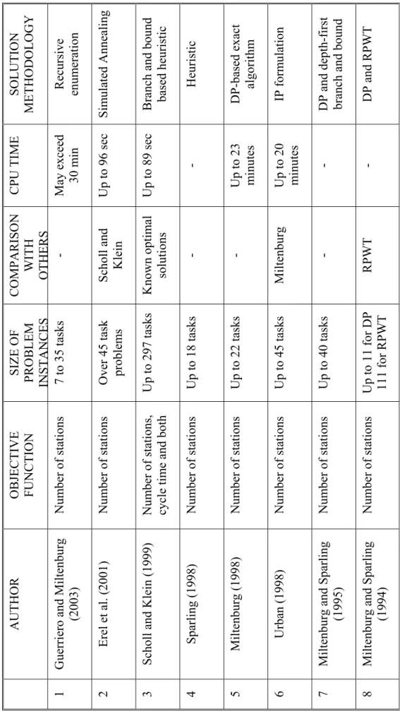
Guerriero and Miltenburg (2003) suggested an exact recursive algorithm for the U-line balancing problem in which the objective is lexicographic minimization first over the number of stations and then over the incompletion probability in the last station. This paper assumes that task times have any distribution function and hence differ from any other work in the literature which assumes deterministic task times. The authors also make computational experiment for problems of size up to 30 tasks. The computation time however, exceeds 30 minutes in some instances. A summary of work done in literature is given in Table 2.2.

26 SOLUTION METHODOLOGY Recursive _enum eration Sim ulated Annealing

Branch and bound based heuristic

Heuristic

DP-based exact

algorithm

IP form

ulation

DP and depth-first branch and bound DP and RPW

T

CPU TIME May exceed 30 m

in Up to 96 sec Up to 89 sec - Up to 23 minutes Up to 20 minutes - - COMPARISON WI T H OTHERS -

Scholl and Klein

Known optim al solutions - - Miltenburg - RPW T SIZE OF _PROBLEM

INSTANCES 7 to 35 tasks Over 45 task problem

s

Up to 297 tasks Up to 18 tasks Up to 22 tasks Up to 45 tasks Up to 40 tasks Up to 11 for DP 111 for RPW

T OBJECTIVE FUNCTION Num ber of stations Num ber of stations Num ber of stations, cycle tim e and both Num ber of stations Num ber of stations Num ber of stations Num ber of stations Num ber of stations AUTHOR

Guerriero and Miltenburg

(2003)

Erel et al. (2001)

Scholl and Klein (1999)

Sparling (1998) _{Miltenburg (1998)} Urban (1998)

Miltenburg and Sparling

(1995)

Miltenburg and Sparling

(1994)

T

able 2.2: Sum

m

ary of work done on paced U-line balancing problem

27

Chapter 3

Proposed Method

3.1 Structure of beam search

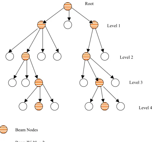
The method proposed to solve the problems stated in chapter 1 is a heuristic based on beam search. Beam search is a fast and approximate branch-and-bound method which operates on a search tree. However it differs from branch-and-bound because a certain number of best paths is selected and the rest is permanently pruned. Thus, at any level in the search tree only the promising nodes are kept for further branching and the other nodes are simply ignored. Beam search moves downward from the best β promising nodes at each level and β is called the beam width. Hence the heuristic is a partial enumeration technique which progresses level by level without backtracking.

In order to select the best β nodes, an estimate of the promise of each node is determined. This value can be determined in various ways: One way is to employ an evaluation function which estimates the minimum total costs of the best solution that can be obtained from the partial design represented by the node. In this case evaluation is based on the global view of the solution. Another approach would be to use one-step evaluation function which may rely on one or several surrogate measures. Unfortunately, there is a trade off between these approaches. One step evaluation is quick but may discard good solutions. On the other hand, a thorough evaluation by the global evaluation function is more accurate but computationally more expensive. Disregarding the complexity of global and local evaluation functions, beam search itself has polynomial time

28 complexity of O(n3) where n is the number of tasks in the problem (Sabuncuoglu

and Karabuk 1998). The running time of the algorithm is polynomial in the size of the problem because a large part of the search tree is pruned off.

A filtering mechanism is also proposed in the literature to reduce the computational effort in beam search. With this mechanism a fast local evaluation function is used to discard some of the nodes based on their local evaluation function values, then only the remaining nodes are subjected to global evaluation. In this approach the number of nodes retained for global evaluation is called the

filter width (α). However we would rather not use this approach because such a good local evaluation function is hard to find and the minimum cost objective is very sensitive to small changes in design. Hence it could be the case that a partial design that is locally evaluated to be bad can prove to be good when globally evaluated.

Figure 3.1: Representation of a beam search tree.

Root Level 1 Level 2 Level 3 Level 4 Beam Width = 2 Beam Nodes

29

In Figure 3.1, a sample beam search tree is shown. We select the best β

number of nodes from the nodes emanating from the root node by comparing the value of the global evaluation function of these nodes. After determining the first beam nodes at level 1, the algorithm is applied to these nodes independently and a partial tree is generated from each of them. Since there are beam width number of nodes in the current level and we progress by keeping one descendant only at each beam node, we have at any level beam width number of nodes and the search progresses from β parallel beams resulting in β different solutions in the end.

Without doubt, the quality of the solutions found by beam search depends both on the beam width β and quality of the global evaluation function.

This search technique was first used by Lowerre (1976) as an artificial intelligence method for the speech recognition problem. Later Fox (1983) used it to solve complex scheduling problems. In another study Chang et al. (1989) used beam search as a part of FMS scheduling algorithm. Sabuncuoglu and Karabuk (1997) developed a beam search based algorithm to evaluate scheduling approaches for flexible manufacturing systems. Leu et al. (1997) used beam search technique for sequencing mixed model assembly lines. Later Sabuncuoglu and Bayiz (1999) applied beam search for job shop scheduling.

Beam search has not been used in the context of assembly line balancing other than sequencing in mixed model lines. Thus, to the best of my knowledge this research is first to use beam search technique for balancing assembly lines. An overview of beam search and its applications can be found in Morton and Pentico (1993).

3.2 Beam search based algorithm for our problem

When using a beam search algorithm there are two important issues to consider: (1) search tree representation and (2) application of a search methodology.

30

3.2.1 Search tree representation

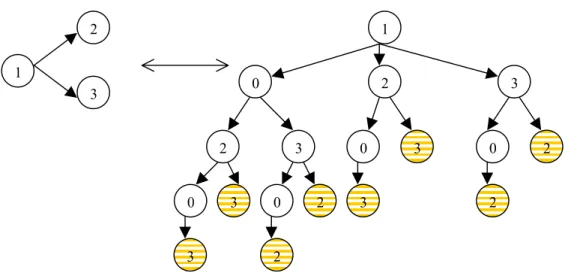
As previously mentioned, each node in the tree corresponds to a partial design. A partial design is an incomplete design where some tasks are allocated to opened stations but there are still tasks to assign and probably more stations to be opened. In this scheme a line between two nodes represents a decision to add a task to the existing station. Since at any level it may be desirable to close the station, we use a dummy task named task 0, the selection of which implies that the current station is closed and a new station is opened. Dummy task can be assigned again and again without being exhausted and is independent of any precedence relations. Once dummy task is assigned at a level, it is prohibited to assign it in the next level because this would mean opening and closing a station without assigning any task to it. Finally, the leaf nodes at the end of the tree correspond to complete designs. To facilitate understanding, the search tree representation of a small precedence diagram is given in Figure 3.2. According to the search tree in Figure 3.2, the path 1-2-0-3 implies that the tasks 1 and 2 are assigned to first station in the given order and task 3 is assigned to second station. The dashed nodes represent the final nodes of their paths.

Figure 3.2: A precedence diagram and corresponding search tree

1 3 2 1 0 2 3 2 3 0 3 0 2 0 3 0 2 3 2 3 2

31

3.2.2 Search methodology

The second issue in beam search is determination of a search methodology. In the proposed algorithm beam search is used to perform search in the tree. No filtering mechanism is used, because filtering mechanism may cause to lose some good solutions for saving from computation time. However, our main concern is the quality of the solutions found rather than reduced computational time. Moreover there is no known filtering mechanism for assembly line balancing problem that is proved to work well. All the nodes at level 1 are globally evaluated to determine the best β number of promising nodes. The selected nodes become the first nodes of the β parallel beams. Subsequently the descendants of these selected nodes are globally evaluated to select the beam node at each parallel beam. If the number of nodes expanded at very first level are less than the specified beam width, then all the nodes in the following levels are expanded until the number of nodes at a level is greater than the specified beam width.

3.2.3 The search procedure

The procedural form of the proposed beam search algorithm is given as follows:

Step 0 :(Initial node generation) Determine the set of available tasks for

assignment considering the precedence relations. These tasks constitute the level 1 nodes. Each node represents a partial design in which the selected task is assigned to the first position in the first station.

Step 1:(checking the number of nodes) If number of level 1 nodes is less than the

specified beam width then expand nodes by generating further level nodes until the total number of nodes in the last level is greater than the specified beam width. Else go to Step 2.

32

Step 2: (completing the partial designs) Since these nodes represent only partially

completed designs, they can't be evaluated globally. In order to evaluate these partially completed designs, they must be completed by assigning the remaining tasks by some heuristic rule. (More on this in the following sections)

Step 3: (computing global evaluation function) Compute the global evaluation

function for all the nodes and select the best β of them. (initial beam nodes) For each beam node:

Step 4: (node generation) Generate descendants of these beam nodes by considering the set of available tasks for that node. Set of available tasks for a node is determined by deducing all up to then assigned tasks for that node from the precedence diagram and choosing the ones with no unassigned predecessors for straight line balancing. For U-line balancing a task must have both its predecessors and followers assigned in order to be available for assignment. Consider also dummy task as the descendant provided that the beam node under consideration has not assigned it in the previous level. (closing the current station)

Step 4.1: (computing global evaluation function) Compute the global evaluation

values of each of these nodes.

Step 4.2: (selecting beam nodes) For each beam in the tree select the node with

the lowest global evaluation value(i.e., beam node). Go to step 2 and proceed until there is no task to assign.

Step 5 : (selecting the solution design) Among the beam width number of designs

generated, select the one with the minimum objective value.

3.3 The evaluation mechanism for straight line

In the beam search based algorithm implemented in this research, when the search procedure comes to evaluate a node, which represents a partial design, it performs two operations. First the line design must be completed by some heuristic rule so that all tasks are assigned to their appropriate stations and secondly this complete design must be evaluated in terms of total expected cost

33 again by some other heuristic or exact procedure. Since this research does not propose any filter mechanisms all the generated nodes are evaluated globally.

3.3.1 Heuristic for completing partial designs

There are several variations of the main heuristic method considered for completing a partially complete design. These variations are all adapted from Kottas, Lau (1973), (1981).

The first heuristic considered is the same heuristic presented by Kottas and Lau (1973) with one slight modification. This heuristic successively builds up stations taking into account the precedence relationships. In order to achieve this, tasks that are available for assignment are classified in desirable list, which comprises tasks, whose placement in the current station increases cost no more than the cost of opening a new station. The selection is then made from sets by some priority rules depending on the status of the station under consideration. This heuristic proceeds in the following manner:

Given a node it first determines the set of assigned tasks and the precedence relations among the remaining tasks. To do this, precedence relationships are preserved for the unassigned tasks but the restrictions arising from tasks that are assigned are no more active. In other words the arcs originating from the tasks that are previously assigned are removed from the precedence diagram.

The very first step in this heuristic is determination of tasks available for assignment. Available tasks must have all their predecessors assigned. Hence if a task has no unassigned predecessor in the precedence diagram it is available for assignment. Such tasks are placed in a set called available list. The heuristic computes available tasks at each step to update the available list. If the available list happens to be empty, this means that there are no more tasks to assign and hence the line design is complete.

The next step in the heuristic is selection of tasks from the available list which are marginally desirable to perform. A task is considered marginally