Robust LQ control for harmonic reference/disturbance signals

Proceedings of the 39" IEEE Conference on Decision and Control Sydney, Australia December, 2000

Robust

L Q

Control for Harmonic Reference/Disturbance

Signals

Hakan Koroglu

Omer Morgul

Bilkent University, Dept. Electrical & Electronics Engineering, Bilkent, 06533, Ankara, Turkey.

Cor. Author: H. Koroglu, Tel.: (90-312) 290-2384, Fax: (90-312) 266-4192, E-Mail: korogluQee. bilkent

.

edu. tr

Abstract

Linear Quadratic (LQ) controller design is considered for continuous-time systems with harmonic signals of known frequencies and it is shown that the design is reducible t o an interpolation problem. All LQ optimal loops are parametrized by a particular solution of this interpolation problem and a (free) stable/proper trans- fer function. The appropriate choice of this free pa- rameter for optimal stability robustness is formulated as a multiobjective design problem and reduced t o a Nevanlinna-Pick interpolation problem with some in- terpolation points on the boundary of the stability do- main. Using a related result from the literature, it is finally shown that, if there is sufficient penalization on the power of the control input, the level of optimum sta- bility robustness achievable with LQ optimal controllers is the same as the level of optimum stability robustness achievable by arbitrary stabilizing controllers. - Keywords : Control design, LQ control, Rm control, Harmonic signals.

1 Introduction

Consideration of harmonic signals in control systems is important from theoretical as well as practical view- points. Theoretical motivation comes from the fact that harmonic signals can be expressed as the superposition of countably many sinusoids. This fact can be utilized to launch a frequency domain approach for the treat- ment of harmonic signals in feedback systems. On the other hand, many engineering systems experience har- monic disturbances. Two common examples are he- licopters experiencing vibrations [l], and disk drives subjected to periodic disturbances [13]. The solutions of the standard control problems of reference tracking and disturbance rejection for deterministic signals uti- lize the (by now classical) Internal Model Principle of [5]. In accordance with this principle, the dynamics of the deterministic signal is replicated in the loop, and the overall design is formulated as the minimization of an appropriate LQ cost. This minimization can then be performed via the state-space methods available for LQ

design (see e.g. [2, 71). An LQ design problem with har- monic signals is considered only recently in [ll], with a formulation similar t o the original LQ problem, by defining the cost directly for the original system. The development is considered for multivariable discrete- time systems and the optimal solutions are described by some interpolation conditions. A much simpler for- mulation of the LQ problem for harmonic signals was done in [9]. The present work extends the development of 191 to achieve some results which can be easily inter- preted and employed in multiobjective design problems. The rest of the paper is organized as follows. In the next section, we describe the setup and give the basic problem formulation of LQ control for harmonic signals (LQH control). In Section 3, we review the internal sta- bility of linear time-invariant (LTI) single-input single- output (SISO) feedback control systems. In Section 4, we show that the problem of LQH control is reducible to an interpolation problem and parametrize all LQH

optimal controllers by a particular solution of this in- terpolation problem and a free stable/proper transfer function. Motivated by this parametrization, we con- sider a multiobjective design problem in Section 5 and develop a robust controller synthesis procedure. After we present a simple example in the penultimate section, we conclude by summarizing our results.

2 Problem Formulation

Throughout the paper, we restrict our attention to SISO and LTI continuos-time systems, though the re- sults are applicable to discrete-time systems with some minor modifications. We consider plants and con- trollers with real rational transfer ,functions. The minor notational preferences are as follows. The space of sta- ble and proper rational functions, H ( s ) , is denoted by

31,

and the well-known

31,

norm is expressed via the standard notation: llHlloo = supw IH(jw)I. Occasion- ally, we treat transfer functions as operators acting on time signals for notational convenience. The complex conjugate of H ( j w ) is shown as H * ( j w ) and the relative degree of H (degree of the denominator minus degree of the numerator) is denoted by p ~ .

d

Y

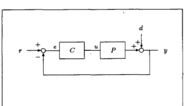
Figure 1: Unity feedback control system.

We consider the unity feedback configuration of Fig- ure 1, where P is the LTI plant and C is the LTI con- troller. The external signals r and d are respectively the reference and the disturbance signals, wheras the internal signals e (= T

-

y) and U are respectively the tracking error and the control input. The infinite hori- zon frequency weighted LQ cost can be defined for SISO continuous-time systems as

[e(t)I2-+ [ F ( s ) u ( t ) I 2 , (1) where F is a LTI stable and minimum phase filter. With the minimization of the LQ cost, the plant output is forced to follow the reference command quadratically optimally with appropriately low control effort. In this paper, we- will study the LQ control problem with har- nals can be expressed as

monic reference and disturbance signals. Harmonic sig-

where wi are the frequencies present in the signal and ai

and 0i are respectively the associated magnitudes and phases. In this setup, the problem of LQH control can be stated as follows:

.

Problem 1 [LQH-Control] Given a LTIplant P and the information that r and d are harmonic-signals with known frequencies (and possibly unknown magnitudes and phases), find a LTI feedback controller C such that the feedback system of Figure 1 minimizes JLQ.

3 Internal Stability Constraints

For simplicity of presentation, we consider in the follow- ing parts of our paper that the plant P has simple strict right half plane poles p i ; i = 1, ..,np and simple right half plane zeros (excluding infinity) zi; i = 1,

..,

n,. We will refer t o p i as unstable poles and to zi as unstable

zeros. With the well-known Blaschke products of poles and zeros are defined as

(3) s - zi nP n. i=l s

+

p ; i=l we can express P as P ( s ) = B*(s)B;1(s)P(s), (4) where is a stable and minimum-phase transfer func- tion. The well known Youla parameter, sensitivity and the complementary sensitivity function of the closed loop system of Figure 1 are defined as

Q ( s ) 4 [ 1 + P ( s ) C ( s ) ] - l C ( s ) , ( 5 )

S(S) 4 [l

+

P ( s ) C ( s ) ] - l

,

( 6 )

T ( s ) 4 [l

+

P ( S ) C ( S > ] - ~ P ( S ) C ( S ) . (7)

It is easy to find that S and T relate to Q as

Q

C ( S ) = T.

S (13)

The system of Figure 1 is internally stable if and only if the functions S , Q, P S and T are all ?t, (i.e. stable and proper) transfer functions [SI. It is well known that this internal stability requirement can equivalently be expressed as some interpolation constraints on the feedback system functions Q, S and T [3, 4, 61). The key observation a t this point is the unacceptability of unstable pole/zero cancellations among P and C . From this we can infer that PC should interpolate t o zero at

z, and to infinity a t p i . It then follows that & ( p i ) = 0,

S ( p i ) = 0 and T ( z i ) = 0, or equivalently

where

a,

and are ?tm transfer functions (see [3]).

Noting that T = PQ (from (4), (9) and ( l o ) ) , and S

+

T = 1 .(from ( 6 ) and (7)), we can write

Bz(s)&)Q(s)

+

B p ( s ) S ( s ) = 1. (11) This relation imposes on Q a group of interpolation constraints which can be expressed as

This way the problem of an internally stable system design is reduced t o finding an

3-1,

transfer function Q

which satisfies (12). After the construction of such a

Q, equation (11) can be solved for S and the feedback controller can be obtained from ( 5 ) and ( 6 ) (after some necessary cancellations) as the minimal realization of

4 LQ Design for Harmonic Signals as an Interpolation Problem

With x defined as

the tracking error and the control input in the feedback system of Figure 1 are determined by

where the relations are expressed in operator notation.

If the control system of Figure 1 is internally stable and

x is a quasi-stationary signal with spectrum

a X x ,

the spectral input/output relations and Parseval's identity (see e.g. [12]) can be used to evaluate the LQ cost as

where ~ L Q can be found (after some straightforward manipulations) to be 2 -1 2 j L Q ( W ) =

(PI' +

1 ~ 1 ~ 1

IQ

- P*

+

IFI2

(pq2

+

p l y .

+

IPI

I

(18) If z is a harmonic signal of the form (Z), 9,, can be found as [12]

where 6 is the well-known Dirac's delta function. Using this in (17) and noting that we are working with real rational transfer functions, we can immediately obtain the expression of the LQH cost ( J L Q with the 2 of (2))

as

Our preliminary result, stated in the following theorem, is a direct consequence of this expression.

Theorem 1 Let the control system of Figure 1 be in- ternally stable and x be a harmonic signal given b y (2).

The feedback loop is LQH optimal (minimizes J L Q H ) if and only if Q , defined according to (lo), satisfies

The optimal LQH cost as given b y

As understood from this theorem, the LQ design for harmonic signals necessitates the determination of a stable/proper transfer function which satisfies the in- terpolation constraints of (21). It is then obvious that Problem 1 is equivalent to the following one.

Problem 2 [Equivalent Problem of LQH Con- trol] Find a transfer function Q E

X,

which satisfies the interpolation constraints given by (12) and (21). This problem can be solved by some standard meth- ods. Given the interpolation data, a stable polynomial of appropriate degree (to satisfy the relative degree re- quirement) can be assigned as the denominator polyno- mial o f f ' and the problem can be reduced t o a polyno- mial interpolation problem, which can be solved by -for example- Lagrange interpolation. Once the equivalent problem is solved, the corresponding controller can be obtained via (13). Obviously there are infinitely many solutions of the LQ design problem for harmonic sig- nals. If &O is a particular solution of the equivalent

problem and B, is the Blaschke product of the har- monics defined as

'

(23) then all LQH optimal controllers can be parametrized as

where H is an arbitrary 7-l- transfer function and

30

is the minimal realization of B;'(l - B,p&). This parametrization describes the whole set of universally optimal (see [ll]) LQH controllers. In other words, the controllers which can be expressed as in (24) optimize

JLQ for any x of the form (2), independent of the mag- nitudes ai and phases

&.

5 Robust LQ Design for Harmonic Signals The principal result of the previous section is the re- duction of an LQ design problem t o an interpolation problem. It is well known that some basic 31, design problems also reduce to interpolation problems (see e.g. [4]). As the LQ design problem of the previous section admits infinitely many solutions parametrized in (24), other design objectives can also be considered. Com- mon framework of treatment with 3-1, control moti- vates us for multiobjective designs in which an 'H, cost is t o be minimized in addition t o the LQH cost. Two

'If wi is zero, the corresponding term in the product should be replaced by s/(s

+

1).

basic problems of

31,

control are the weighted sensitiv- i t y minamization problem and the stability robustness optimization problem [4]. We consider below the sta- bility robustness optimization problem together with LQH minimization.

Stability robustness optimization (for additive plant perturbations) in an

31,

setting considers the mhi- mization of the cost

(25) where W is a stable, proper and minimum phase trans- fer function (see [3]). This problem (as well as some other

X,

control problems) is closely related with the Nevanlinna-Pick interpolation problem (see [4]).

Nevanlinna-Pick interpolation problem (in its classi- cal formulation) considers the determination of transfer functions in

X,,

which satisfy a group of interpola- tion constraints at given strict right half plane points and which have

31,

norms less than or equal t o unity. The stability robustness optimization problem reduces to such a problem as a result of the internal stability constraints imposed by the unstable poles. If we define

G as

we can replace

Jx,

with

llGll,,

as we have IBp(jw)I = 1. It follows from (26) and (12) that G E Z,

G(s) W ( 4 Q ( s ) , (26)

1,

{ H E

31,

: H ( p i ) = ai;Vi;i=l,..,n,.}, (27) and CY( 's are defined as

ai W(pi)B,'(pi)P-' ( p i ) ; i = 1,

..,

np. (28)

If the relative degree of W is greater than zero, we should also impose p~ = pw. Yet, independent of the relative degree constraint on G, the optimum value of

Jx,

is equal to the maximum lower bound of the

31,

norms of the transfer functions in

I,,

which we define as

It is well known from classical theory [4, 81 that ? ( I p ) is given by

where A and B are the matrices defined as

and Amax denotes the maximum eigenvalue. If we scale the interpolation data with 7 - ' ( Z P ) , we end up with the classical Nevanlinna-Pick interpolation problem, for which we have closed form solutions [S] as well as itera- tive construction algorithms [3, 41. The relative degree

constraint leads to a technical hindrance in 31, opti- mization. For this reason, usually the optimum cannot be achieved by proper controllers. Yet it can be ap- proached arbitrarily by an appropriate modification of

the optimal (improper) controller [3, 41.

The observation that optimization can also be treated in the interpolation framework motivates us for the following multiobjective design problem:

Problem 3 [Robust LQH Control] Given a LTI plant with simple unstable poles and zeros having positive real parts, determine among the LQH op-

timal controllers of (24) the one which minimizes

IIW(S)QLQH(S)II, for a stable, proper and minimum phase transfer function W .

Among the transfer functions G E Z,, the ones corre- sponding t o an LQH optimal loop are in 1,where

{ H E

31,

: H ( j w i ) = ,&;W;i=l, ..,nu.}

,

(32)

5

and pi's are defined as

In other words, for LQH optimality we should have G E Zp

n I,.

This means that we can state the equivalent problem of robust LQ control for harmonic signals as follows.

Problem 4 [Equivalent Problem of Robust LQH

Control]

Given

a LTI

plant

with

sample unstable poles/zeros having positive real parts, and a stable, proper and minimum phase transfer function W , find a

transfer function G E TpnZw of relative degree PG = pw

such that llGll, is (arbitrarily close to its) minimum.

It follows from the discussion above that, the determi- nation of the optimum cost necessitates the use of the Nevanlinna-Pick theory. Due t o the presence of interpo- lation points on the boundary of the stability domain (which is the imaginary axis for our case), the stan- dard theory (which assumes no boundary interpolation points) is not applicaple. An extended treatment of the Nevanlinna-Pick problem t o include boundary interpo- lation points is done by Khargonekar and Tannenbaum in [8]. For the sake of completeness, we cite below their relevant result with necessary adaptations.

Theorem 2 ([SI) Let pi be distinct strict right plane points and jwi be distinct imaginary axis points. Let the sets (of transfer functions) 1,and Z, be defined by (27) and (32). The maximum lower bound for the

31,

norms of the transfer functions in 1,

n

Z, is given b y

Application of this result to our case gives us the bound on the maximum attainable stability robustness to- gether with LQ optimality for harmonic signals. The result also has an important implication concerning the simultaneous optimization of JLQH and

Jx,

.

Before we present this as a theorem, we define a new cost JRLQH

as

JRLQH JLQH

+

Jxa.

(35) The following theorem, which states an important re- sult on the minimization of JRLQH, is a direct corollary

of Theorem 2.

T h e o r e m 3 Let P be a plant with simple unstable poles (pi) and zeros (zi) with positive real parts, and let Z, and y(Zp) be defined as in (27) and (29).

If

F satisfies

for all i = 1, ..,nu, then the infimum of JRLQH is given

b y inf JRLQH =

J;gH

+

inf Jx,

.

R e m a r k 1 Conditions given by (36) determine the best achievable level of tracking/rejection for a har- monic signal of known frequencies, if stability robust- ness optimization is the principal concern. It also shows

the significance of the presence of the frequency weight- ing filter in the LQ cost (which was mainly for the pe- nalization of the power of the control input) from the aspect of stability robustness.

Obviously the optimum of our multiobjective design problem is generally unattainable due to the relative degree constraint and the degeneracy imposed by the interpolation conditions at the harmonics. Yet any (slightly) greater cost, which is arbitrarily close to the optimum, is achievable (similarly to the

31,

optimiza- tion). We outline below a procedure, with which such solutions can be constructed.

P r o c e d u r e 1 [Robust LQH Design] Given P , F ,

W and wi; 1. 2. 3.

4.

5. 6.

Determine y(Z,

n

Tu)

using (30) and (34).

Find G E

z,ng

such that

llG1103

5

y(ZpnZu)+c

with (arbitrarily small) c

>

0.

Modify G as G

+

G ( l

-

B p B u ( ~ s ) / ( ~ s

+

l ) ) P w

with (arbitrarily small) E

>

0. Set QRLQH = W-IG.

Set SRLQH(S) as the minimal realization of

B

;

'

(1

-

B, PQR LQH).

Obtain CRLQH as CRLQH = QRLQH/SRLQH.

The second step of this procedure necessitates a Nevanlinna-Pick interpolation algorithm that can treat boundary interpolation points. Such an algorithm can be found in

[lo].

Actually, the algorithm of

[lo]

can also cope with unity relative degree requirement, and this might be useful in obtaining low degree controllers. If G is constructed to have a certain relative degree, the third step of the algorithm should b e modified accord- ingly.

6 I l l u s t r a t i v e Design E x a m p l e

We illustrate the robust LQ design with harmonic sig- nals for a simple plant with transfer function P = l / ( s - 1 ) . Clearly, we have

B,

= 1, Bp = ( 5 - l ) / ( s + l )

and P = l / ( s

+

1). The internal stability constraint on Q is simply Q ( l ) = 2. With -W = (s

+

0.2)/(s

+

1)2, the infimum of (25) is W ( l ) Q ( l ) = 0.6 and thus the minimizing G is simply 0.6 (see [4]). This solution cannot be achieved by any proper controller (as the required relative degree for G is unity), yet can arbi- trarily be approached. If robust LQH design is consid- ered for frequencies wi = {0.5,1,2}, conditions of (36) are (just) satisfied by F(0.5j) = 0, F ( j ) = 0.3177 and

F ( 2 j ) = 0.3156, Assuming a denominator polynomial of (s

+

1)6 for Q, and finding the appropriate numera- tor polynomial to satisfy (12) and (21), we can obtain a particular LQH optimal controller as

cLQH

(s) = 8.993se+ll.O5s5+45.2s4+22.08s5+32.93s2+4.376s+3.376 s6 - 0 . 9 9 2 9 ~ ~ +8.962~4 - 1.241~3 +11 .68s2 -0.2482s+2.376

Applying the procedure for robust

LQH

design (by making use of the algorithm of [lo] with relative degree treatment), we can construct a robust LQH controller with c = 0.05 as

. . .

+14.33s2+14.74s-0.0819 +0.6084s2 +9.926s-0.1071

The magnitude variation of W Q correponding to the optimally robust loop, LQH optimal loop and robust LQH optimal loop are are displayed in Figure 2. As the figure shows, WQRLQH has a similar magnitude varia- tion with the W Q x , except at the harmonics and the high-pass band. The

31,

norm of WQRLQH is 0.65. If CRLQH is constructed with a smaller c, the varia- tions will look more similar and the

3-1,

cost of CRLQH

will be closer to 0.6, however the numerical sensitiv- ity of the synthesis algorithm does not allow extremely small E ' S . Moreover, the results of the simulations per-

formed with a harmonic disturbance and zero reference (see Figure 3) show that, the robust LQH controller has a poor transient behaviour (control is started af- ter the second period). With smaller e 's, the transient response gets worse. This is the most remarkable trade- off in the robust design.

I I _{Acknowledgements: We would like to express our}

sincere thanks to Prof. Hitay Ozbay and Prof. Peter Dorato for supplying us some references and comment- ing on our work.

Figure 2: Magnitude Msiation of WQ (WQRLQH : solid, W Q L Q H : dashed, W Q x , : dash-dotted).

I

*.a 60 Im 760 200 160 PO

-

ua

$(- I

Figure 3: Simulation results with wi = {0.5,1,2}, ai = {1,0.5,0.3} and Oi = 0 (CLQH : top, CRLQH : bottom).

7 Conclusions

We considered the LQ design problem for linear time- invariant continuous-time systems with harmonic sig- nals of known frequencies and showed that the de- sign is reducible to an interpolation problem. We then parametrized all LQH optimal controllers in terms of a particular LQH optimal solution and a free parameter. The choice of this free parameter t o obtain a desired overall closed-loop behaviour motivated a multiobjec- tive design problem, in which an

31,

cost as well as the LQH cost is to be minimized. Here we considered the stability robustness optimization together with LQ optimization for harmonic signals and showed that this problem is reducible to a Nevanlinna-Pick interpolation problem with some interpolation points on the bound- ary of the stability domain. If the frequency weighting filter in the LQ cost has sufficiently great magnitudes a t the harmonics under consideration, the optimal robust stability level can arbitrarily be approached while si- multaneously satisfying the LQH optimality conditions. This result finds its use in a design procedure in which stability robustness is the principal concern and track- ing/rejection of the harmonic signals is the secondary aim. Our results apply to discrete-time systems with some minor modifications. Several other 31, design problems (e.g. weighted sensitivity minimization, gain margin optimization) can be considered together with LQ optimal design for harmonic signals and they can be solved via similar interpolation methods.

'

References

[l] S. Bittani, F. Lorito, and S. Strada. An LQ ap- proach t o active control of vibrations in helicopters.

ASME Journal of Dynamic Systems, Measurement, and Control, 118(3):482-488, 1996.

[2] E. J. Davison and P. Patel. Application of the robust servomechanism controller t o systems with peri- odic tracking/disturbance signals. International Jour- nal of Control, 47(1):111-127, 1988.

[3] P. Dorato, L. Fortuna, and G. Muscato. Robust Control for Unstructured Perturbations: A n Introduc- tion. Springer-Verlag, NY, 1992.

[4] J. C. Doyle, B. A. Francis, and A. R. Tannen- baum. Feedback Control Theory. Macmillan Publishing Company, NY, 1992.

[5] B. A. Francis and W. M. Wonham. The Inter- nal Model Principle of control theory. Automatica,

[6] J. W. Helton and 0. Merino. Classical Control Using

31,

Methods: Theory, Optimization, and De- sign. SIAM, NY, 1998.

[7] A. Iftar. Optimal solution t o the servomecha- nism problem for systems with stochastic and deter- ministic disturbances. International Journal of Control, 51(6):1327-1341,1990.

[SI P. P. Khargonekar and A. R. Tannenbaum. Non- Euclidian metrics and the robust stabilization of sys- tems with parameter uncertainty. IEEE Transactions on Automatic Control, AC-30(10):1005-1013, 1985. [9] H. Koroglu and 0. Morgiil. LQ optimal design at countably many frequencies. In Proceedings of the 37th IEEE Conference on Decision and Control, pages 1195-1196, Tampa, Florida, USA, December 1998.

[lo] Y. Li. U-Parameter Design: Feedback System De- sign with Guaranteed Robust Stability. PhD thesis, De- partment of Electrical and Computer Engineering, Uni- versity of New Mexico, February 1989.

[ll] A. Lindquist and V. A. Yakubovich. Universal regulators for optimal tracking in discrete-time systems affected by harmonic disturbances. IEEE Transactions on Automatic Control, AC-44(9):1688-1704, 1999. [12] L. Ljung. System Identification: Theory for the User. Prentice-Hall, Englewood Cliffs, N J , 1987. [13] A. Sacks, M. Bodson, and P. Khosla. Experimen- tal results of adaptive periodic disturbance cancellation in a high performance magnetic disk drive. ASME Jour- nal of Dynamic Systems, Measurement, and Control,

12(5):457-465, 1976.