WITH TRANSPORTATION CAPACITY
a thesis
submitted to the department of industrial engineering
and the institute of engineering and science
of bilkent university
in partial fulfillment of the requirements
for the degree of
master of science
By
Nasuh C
¸ a˘gda¸s B¨uy¨ukkaramıklı
December, 2006
Prof. ¨Ulk¨u G¨urler (Advisor)
I certify that I have read this thesis and that in my opinion it is fully adequate, in scope and in quality, as a thesis for the degree of Master of Science.
Asst. Prof. Osman Alp (Co-advisor)
I certify that I have read this thesis and that in my opinion it is fully adequate, in scope and in quality, as a thesis for the degree of Master of Science.
Asst. Prof. Alper S¸en
I certify that I have read this thesis and that in my opinion it is fully adequate, in scope and in quality, as a thesis for the degree of Master of Science.
Asst. Prof. Pelin Bayındır
Approved for the Institute of Engineering and Science:
Prof. Mehmet B. Baray Director of the Institute
ECHELON INVENTORY SYSTEMS WITH
TRANSPORTATION CAPACITY
Nasuh C¸ a˘gda¸s B¨uy¨ukkaramıklı M.S. in Industrial Engineering
Supervisor: Prof. ¨Ulk¨u G¨urler , Asst. Prof. Osman Alp December, 2006
In this study, we examine the stochastic joint replenishment problem in the pres-ence of a transportation capacity. We first study the multi-retailer and single-echelon setting under a quantity based joint replenishment policy. A limited fleet of capacitated trucks is used for the transportation of the orders from the ample supplier in our setting. We model the shipment operations of the trucks as a queueing system, where the customers are the orders and trucks are the servers. Consequently, different transportation limitation scenarios and meth-ods of approach for these scenarios are discussed. We then extend our model to a two-echelon inventory system, where the warehouse also holds inventory. We characterize the departure process of the warehouse inventory system, which becomes the arrival process of the queueing system that models the shipment operations between the warehouse and the retailers. This arrival process is then approximated to an Erlang Process. Several numerical studies are conducted in order to assess the sensitivity of the total cost rate to system and cost parameters as well as the performance of the approximation.
Keywords: Stochastic Joint Replenishment Problem, Queueing Theory,
Trans-portation Limitation, Inventory Theory. iii
ULASIM KISITLI ˙IK˙I D ¨
UZEYL˙I ENVANTER
S˙ISTEMLER˙INDE TOPLU S˙IPAR˙IS¸ PROBLEM˙I
Nasuh C¸ a˘gda¸s B¨uy¨ukkaramıklı End¨ustri M¨uhendisli˘gi, Y¨uksek Lisans
Tez Y¨oneticisi: Prof. Dr. ¨Ulk¨u G¨urler , Yard. Do¸c. Dr. Osman Alp Aralık, 2006
Bu ¸calı¸smada ula¸sım kapasiteli envanter sistemlerindeki toplu sipari¸s problemi incelenmi¸stir. Once tek d¨uzeyli ¸cok perakendecili bir ortamda miktar bazlı¨ toplu sipari¸s politikaları incelenmi¸stir. Sipari¸slerin, kapasitesi sınırsız olan bir tedarik¸ciden perakendeciye ta¸sınmasında kapasiteli kamyonlardan olu¸smu¸s bir filo kullanılmaktadır. Toplu sipari¸slerin kamyonlar tarafindan ta¸sınması i¸slemleri, kamyonların birer i¸sgoren, sipari¸slerin de birer m¨u¸steri oldu˘gu bir kuyruk sis-temi ile modellenmi¸stir. Bu model altında sisteme ait toplam maliyet fonksiy-onu yazılmı¸s, farklı ula¸sım kısıtı senaryoları i¸cin ¸ce¸sitli ¸c¨oz¨um yakla¸sımları geli¸stirilmi¸stir. Daha sonra model, tedarik¸cide de envanter tutulan iki d¨uzeyli bir envanter sistemine geni¸sletilmi¸stir. Depo envanter sisteminin ¸cıkı¸s s¨urecinin, depo ile perakendeciler arasındaki ta¸sıma sisteminin modellenmesinde kullanılan kuyruk sisteminin giri¸s s¨urecine e¸sde˘ger oldu˘gu g¨ozlemlenmi¸s ve bu s¨ure¸c karak-terize edilmi¸stir. Bu giri¸s s¨urecini bir Erlang s¨ureci ile yakla¸sıklayarak, sisteme ait toplam maliyet fonksiyonu t¨uretilmi¸stir. Yapılan yakla¸sıklamanın perfor-mansını ¨ol¸cmek ve sistem parametrelerinin duyarlılı˘gını g¨ozlemlemek amacıyla ¸ce¸sitli sayısal ¸calı¸smalar y¨ur¨ut¨ulm¨u¸st¨ur.
Anahtar s¨ozc¨ukler : Rassal Toplu Sipari¸s Problemi, Kuyruk Kuramı, Ula¸sım
Kısıtlamaları, Envanter Kuramı.
First and foremost, I would like to express my sincere gratitude to my supervisors Prof. ¨Ulk¨u G¨urler and Asst. Prof. Osman Alp for their concern and guidance during my M.S. study. They have been always ready to provide help, support and trust. I have learned a lot of things from them, not only in academic but also in personal and intellectual matters. I consider myself lucky to have worked under their supervision.
I would like to thank to Asst. Prof. Alper S¸en and Asst. Prof. Pelin Bayındır for accepting to read and review this thesis and their substantial comments and suggestions.
Also, I would like to express my gratitude to TUBITAK for its financial sup-port throughout my Master’s study.
I am indebted to Banu Y¨uksel ¨Ozkaya for her academic and morale support at all times. She has always provided help even when she was very far away.
I want to thank ¨Onder Bulut, Ahmet Camcı and Sıtkı G¨ulten. It would have been very hard without their comradeship.
I indebted to my dear friends Nurdan Ahat, Ay¸seg¨ul Altın, C¸ i˘gdem Ataseven, Didem Ekmek¸ci, C¸ a˘grı Latifo˘glu and Berkay Toprak for their morale support. Also, I want to thank to all of my office-mates for their understanding as well as to all of the friends that I failed to mention here.
Finally, I would like to express my deepest gratitude to my family for their everlasting love and support.
1 Introduction and Literature Review 1
2 Single-Echelon Environment 9
2.1 Model Characteristics . . . 9
2.2 Preliminary Analysis . . . 12
2.3 Derivation of the Operating Characteristics . . . 14
2.3.1 Derivation of the Waiting Time Distribution of an Order for a Truck . . . 18
2.3.2 Objective Function . . . 20
2.4 Analysis of the Total Cost Rate Function . . . 22
2.5 Different Scenarios and Solution Procedures . . . 25
2.6 Numerical Study . . . 28
3 Two-Echelon Environment 33 3.1 Model Characteristics . . . 33
3.2 Preliminary Analysis . . . 36
3.2.1 General Characteristics of the Departure Process of a (S − 1, S) Inventory System . . . . 38 3.2.2 Analysis of the Shipment Operations of the Retailer Orders
at the Truck Base . . . 42 3.3 Derivation of the Operating Characteristics . . . 46 3.4 Numerical Study . . . 48
3.4.1 Sensitivity of the Total Cost Rate to Cost and System Pa-rameters . . . 48 3.4.2 Accuracy of the Approximation . . . 54
4 Conclusion and Future Studies 57
A Algorithms Part 64
A.1 Accuracy Check Algorithm . . . 64 A.2 Search Algorithms for Different Types of Transportation
Limita-tion Scenarios . . . 65
B Proof Part 68
2.1 Illustration of the environment . . . 10 2.2 Realization of the model . . . 13 2.3 Illustrations of how backordering and holding costs per unit are
incurred . . . 15 2.4 Illustration of the change of AC(Q, (S∗(Q, K)), K, C) in K . . . . 23 2.5 Illustration of the change of AC(Q, (S∗(Q, K)), K, C) in Q for a
given K . . . . 24 2.6 Illustration of the change of AC∗, S∗ and Q∗/C with λ
0 . . . 31
3.1 Illustration of the extended model . . . 34 3.2 Illustration of the Shipment Operations of the Retailer Orders . . 36 3.3 Illustration of the Consecutive Demand Departures . . . 39 3.4 Comparison of the Erlang Approximation with the Queue
Inter-arrival Times . . . 44 3.5 Comparison of the Erlang Approximation with the Queue
Inter-arrival Times . . . 45 3.6 Illustration of the change of AC∗% with Q . . . . 50
3.7 Illustration of the change of AC∗ with K for different C . . . . 51
3.8 Illustration of the change of the difference between simulated AC and approximated AC with ρ . . . . 56
2.1 The Effects of the Change in a = A(C)/C and K on Total Cost Rate . . . 28 2.2 The Effects of the Change in βi and K on Total Cost Rate . . . . 29
2.3 The Effects of C and K on Total Cost Rate for C = 2, 4, 8, 16 and 32 . . . 30 2.4 The Effects of K on Optimal Cost Parameters for different N . . 32 3.1 The Effects of the Change in A(C) and K on Total Cost Rate . . 49 3.2 The Effects of the Change in βi and K on Total Cost Rate . . . . 52
3.3 The Effects of the Change in D and K on Total Cost Rate and Other System Parameters . . . 53 3.4 The Effects of λ0 on AC∗ and Other System Parameters . . . 53
3.5 The Impacts of Lwh on AC∗ and Other System Parameters . . . . 54
3.6 The Accuracy of the Approximation for different ρ . . . . 55
Introduction and Literature
Review
Current research trend in logistics management stresses the importance of in-tegration of different functional operations within a firm throughout the supply chain. By the integration of the supply chain, many companies have succeeded in reducing costs and increasing service levels. Recent advances in the infor-mation technology enable the sharing of available inforinfor-mation among different parts of the supply chain more effectively, which facilitates the coordination of the different functional areas within a firm.
Inventory and transportation costs comprise the bulk of the total operating costs of a distribution system. Substantial reduction in total costs is achiev-able by incorporating transportation and inventory control decisions carefully. In general, there is a trade-off between the inventory and transportation costs in a logistics system. Hence, coordinated planning of the inventory and transportation decisions can greatly reduce the total operating costs of the system.
In this study, we focus on coordinated replenishment policies in single-echelon and two-echelon single-item/multi-location inventory settings under transporta-tion capacity. In particular, we study Stochastic Joint Replenishment Problem (SJRP) in settings, where transportation is capacitated.
SJRP is the determination of replenishment and stocking decisions for dif-ferent items (or retailers) to minimize total expected operating (i.e. holding, shortage and order setup/transportation) costs per unit time, when demands are random and joint ordering cost structures are present. In most of the real world systems, the ordering cost structure presents an opportunity to benefit from the economies of scale in replenishment by giving orders jointly. This is possible when the items are purchased from the same supplier or they share the same transportation vehicle.
In most of the distribution systems, the transportation of items are capac-itated. Most of the firms have their own limited fleet for their transportation operations. (e.g. Shell, BP, etc...), whereas some of the firms contract with a 3PL provider for running of their transportation operations. In both of the cases, the transportation is not unlimited. The fleet size and the capacity of the trucks have their own kind of cost structures. Hence, the size of the fleet that is used in the transportation of the orders and the capacity of the vehicles are also the challenging decisions companies have to make. So, considerable cost savings can be achieved by coordinating the joint replenishment policy decisions with these aforementioned transportation related decisions in the supply chain systems.
The stochastic joint replenishment problem (SJRP) differs from the determin-istic joint replenishment problem greatly in modelling methodologies and policy structures. We refer the reader to Aksoy and Ereng¨uc [1] and Goyal and Satir [20] for the extensive review of the works about the deterministic JRP .
To our knowledge, Ignall [23] is the only study that analyzes the optimal joint replenishment policy in the SJRP . The optimal policy, even for a two-item case and zero lead-times has a very complicated structure. As the number of items in the system increases, the structure of the optimal policy would be more complicated. Therefore, the control and the implementation of the optimal joint order policies in practice would be even more challenging. This is one of the main reasons why most of the existing studies in the literature is mostly focused on finding and evaluating intuitive heuristic policy classes, which are easier to control and implement in practice.
Balintfy [6], which is the earliest study in the stochastic joint replenishment problem literature, develops a continuous-review joint ordering policy: (S, c, s), which is referred to as the can-order policy. This policy determines the reorder, s = (s1, s2, ..., sN) and can-order, c = (c1, c2, ..., cN) points as well as the order
up-to levels, S = (S1, S2, ..., SN) for each item i. The policy operates as follows:
a demand to item i triggers a replenishment order whenever the inventory po-sition of that item drops to its reorder point si. After the replenishment order,
the inventory position of item i is increased to its order up-to level Si. At the
same time, any other item j whose inventory position is less than or equal to its can-order point, cj (sj < cj < Sj) is also included to the joint replenishment
order, and their inventory positions are raised to their order up-to levels Sj. The
implementation of the policy seems to be simple, however the calculation of op-erating characteristics under this policy is very difficult, even in the presence of unit Poisson demands.
Silver [34] studies a special case of the can-order policy. In his study, the lead-time is zero, the items face unit Poisson demands, shortages are not allowed and c = S-1 and s=0. With the objective of minimizing the expected total cost per unit per time, Silver [34] proves that the can-order policy performs better than the individual control policy if the cost of ordering an item is equal to that of ordering two items jointly. If these ordering costs are not equal, he shows that there exists a critical value for the fixed item ordering cost above which joint replenishment policy becomes more profitable compared to individual replenishment policy.
Silver [36] also develops a new approximation technique for the analysis of the can-order policies. In this approximation technique, the N-item problem is decomposed into N single-item problems. This single-item problem is first ana-lyzed by Silver [35] and solved optimally by Zheng [44]. Subsequently, Thompson and Silver [39], Federgruen et al. [16], Silver [37], Van Eijs [42] and Schultz and Johansen [33] focus on the different aspects of can-order type policies.
the size of the optimization problem (for an N-item setting, can-order policy em-ploys 3N policy parameters) call for the need for more parsimonious continuous-review control policies.
The continuous-review (Q, S) policy, one of the most frequently used policies in the industry, is first proposed by Renberg and Planche [30]. In this policy, whenever a total demand of Q units accumulate for all items, a joint order of size
Q is given to the supplier, and the inventory positions of each item is raised to
the vector of order-up-to levels S=(S1, S2, ..., SN). This policy uses N + 1 policy
parameters for an N-item setting. Pantumsinchai [29] subsequently presents the exact analysis of the (Q, S) policy and compares the performance of it with that of (S, c, s) policy. The numerical results indicate that the (Q, S) policy performs better than the can-order policy if the fixed ordering cost is high and the backorder cost is low, whereas the can-order policy only performs better if the fixed ordering cost is low.
Atkins and Iyogun [2] suggest two periodic review replenishment policies for unit Poisson demands. In the first proposed policy, which is referred as P , inven-tory positions of all items are raised to their order up-to levels S at the end of each period of length T . In the second policy, which is represented by MP , the review periods are integer multiples of a base period and review periods can differ for each item. From the numerical results, Atkins and Iyogun [2] assert that P and MP type policies outperform the (S, c, s) policy as the fixed ordering cost increases.
Nielsen and Larsen [26] suggest a new policy referred to as the Q(S, s) policy. This policy functions as follows: whenever a total demand of Q units are accu-mulated since the last review, a replenishment order is triggered and the items whose inventory positions at or below s in this review epoch are raised to their order-up-to levels S.
Cachon [10] proposes a new policy for the dispatchment of the trucks in a single-echelon distribution system, and compares the performance of this new policy with those of (Q, S) and P type policies. This new policy, which is referred to as the (Q, S|T ) policy operates as follows: the retailer reviews its inventory
every T time units and trucks are dispatched if the accumulated retailer orders can fill the trucks in such a way that one of the trucks has at least Q units and others are full. Note that Q can take a value less than or equal to the truck capacity in this particular policy.
In a recent study, ¨Ozkaya et. al [28], suggest a new parsimonious policy for unit Poisson demands as well as for the batch demands. This policy, which is referred to as (Q, S, T ) policy, is a sort of hybrid of the continuous review (Q, S) and periodic review P policies. It performs as follows: the items are reviewed continuously and the inventory positions of all items are raised to S = (S1, S2, ..., SN) whenever a total Q demands accumulate for the items or T time
units have elapsed, whichever occurs first. It is shown numerically that (Q, S, T ) policy performs better than the other joint replenishment policies under most of the settings. Next, we elaborate on the multi-echelon joint replenishment literature.
There is a vast literature on multi-echelon inventory systems. For a general review of the literature, the reader is referred to Federgruen [15]. The analytical treatment of the policies for the SJRP in two-echelon inventory systems is more difficult compared to single-echelon inventory systems. Therefore the studies about SJRP in single-echelon inventory systems outnumber the studies in multi-echelon inventory systems. Among the related works, Axs¨ater and Zhang [5] and Cheung and Lee [13] study the SJRP for continuous review models in two-echelon divergent inventory systems.
¨
Ozkaya [27] provides a modeling methodology for a general policy class for the SJRP in two-echelon inventory systems. Via this modeling methodology, she analyzes most of the joint replenishment policies in the literature in two-echelon distribution systems and compares the performance of these policies in various parameter settings.
Lastly, we mention about Vendor Managed Inventory (VMI) systems, which is a related topic in the multi-echelon inventory management. The recent studies by C¸ etinkaya and Lee [11] and Kiesm¨uller and de Kok [24] focus on different aspects of consolidation policies in the V MI systems. In the V MI systems, small retailer
orders are combined to larger shipments at the warehouse level according to a consolidation policy. In most of the V MI literature, the problem is analyzed from the warehouse perspective, though the impact of the consolidation policies on the retailers’ performance is mostly neglected.
Existing literature in SJRP overlooks some important transportation matters such as the effects of a limited fleet size and cargo capacity constraints. To our knowledge, Cachon [10] and G¨urb¨uz [21] are the only studies that incorporate the truck capacity considerations with the analysis of the joint replenishment policies, but in their studies, they both assume that there is an unlimited availability of transportation vehicles. However, unlimited availability of transportation vehicles is not possible in most of the real life applications. Therefore, the transporta-tion limitatransporta-tion problem has been analyzed in the supply chain literature both in deterministic and stochastic demand cases. In some of these studies, system parameters are optimized for a given truck capacity and/or fleet size, whereas there are some studies, where they are taken as decision variables, too. Next, we briefly review the relevant supply chain literature on the transportation limitation problem.
In both deterministic and stochastic demand cases, there are various models that handle the truck/cargo capacity problem under the assumption of an unlim-ited fleet size similar to Cachon [10]. In such a case, truck capacity constraint greatly determines the ordering cost structure of the system.
In the deterministic demand case, Toptal et al.[41], C¸ etinkaya and Lee [12] study different types of coordination problems in the presence of cargo capac-ity constraints. Also, Benjamin [8] considers a joint production, transportation and inventory problem with deterministic demand, allowing supply capacity con-straints.
In the random demand case, Yano and Gerchak [43], Henig et al. [22] and Ernst and Pyke [18] analyze different types of models with the truck capacity consideration. Note that truck capacity is also considered to be one of the decision variables in these aforementioned studies.
In the literature, fleet size consideration is generally taken into account in inventory-vehicle routing problems. Ball et al. [7] address the problem of finding an optimal fleet size as well as determining the vehicle routes where the demand is deterministic. In the stochastic demand case, Federgruen and Zipkin [17] study an integrated vehicle routing and allocation problem with a given fleet of capacitated vehicles. For a broader review of inventory-vehicle routing problems, we refer the reader to Dror and Ball [14] and Ben-Khedher and Yao [9].
In a recent paper, Sindhuchao et al.[38] develop a mathematical programming approach for the multi-item joint replenishment problem in an inventory-routing system with a limited vehicle capacity. In this study, the demand is assumed to be deterministic. Although the motivations behind this work are parallel to ours, the methodology of the approach differs greatly in our problem due to the random demand structure.
In this study we study a specific kind of a control policy for the SJRP, which is (Q,S) policy, in the presence of a truck capacity and fleet size limitation in both single and two-echelon divergent multi-retailer systems with unit Poisson demands. To our knowledge, our study is the first one that incorporates the decisions of the truck capacity and fleet size in the stochastic joint replenishment problem.
The shipment operations of the trucks is modelled as a queueing system, where the customers are the orders and trucks are the servers. By using some of the key results in the queueing theory, we derive the operating characteristics of the single-echelon inventory systems in the presence of the limited fleet size of the capacitated trucks analytically. We investigate the characteristics of the total cost rate function and construct methods of approach for different kinds of transportation limitation when there is a maintenance/depreciation cost rate factor per truck. We also present the results of our numerical study to assess the sensitivity of decision variables to the system parameters.
The analysis for the single-echelon inventory system is extended to a two-echelon system, where the upper two-echelon also holds inventory. In this two-two-echelon
system, a joint retailer order has to be satisfied by the warehouse inventory sys-tem before it is dispatched by the trucks. Since the operations of the trucks are modeled as a queueing system, the departure process of the warehouse inventory system constitutes the arrival process for this queueing system. This problem in our setting leads us to a more general problem, and we derive the general characteristics of the departure process of an (S-1, S) inventory system where the arrivals occur according to a renewal process. From these general results, we obtain the first two moments of the inter-departure times of the warehouse inven-tory system. Working with the original departure process, which has dependent increments is analytically intractable due to its complicated nature, therefore, we approximate the departure process to an Erlang Process, and derive the operat-ing characteristics of the system accordoperat-ing to this approximation. We compare the approximation results with the simulation results and present the sensitivity of the system to the decision and system variables in the numerical study part. We observe that our approximation method works fairly well except for very high traffic rate. (ρ > 98%)
The remainder of the thesis is organized as follows:
In Chapter 2, we analyze the SJRP with transportation limitation in the single-echelon inventory systems. In Chapter 3, the analysis is extended to a two-echelon inventory system, where the upper two-echelon also holds inventory. Finally, in Chapter 4, we conclude the thesis by giving an overall summary of our work, our contribution to the existing literature and its practical implications with future research directions.
Single-Echelon Environment
In this chapter we present an analytical model for the coordination of inventory and transportation decisions in a single echelon, single item, multi-retailer dis-tribution system under transportation capacity. Main assumptions of the model are presented in Section 2.1. Section 2.2 presents a preliminary analysis, which is followed by the derivation of the expressions for the key operating character-istics and the statement of the optimization problem in Section 2.3. In Section 2.4, we discuss some of the characteristics of the total cost rate function of the system, which we use in Section 2.5, while constructing the search algorithms according to different scenarios of transportation limitation. Finally in Section 2.6, we present the numerical results, where we assess the total cost rate of the system with respect to the system parameters.
2.1
Model Characteristics
We consider a single item, multi-retailer inventory setting under continuous re-view. (The model presented in this Chapter can be easily adopted to a multiple-items/single-retailer setting). The retailers face stationary and independent unit Poisson demands with rate λi (i = 1, 2, ..N ), and all unmet demands are fully
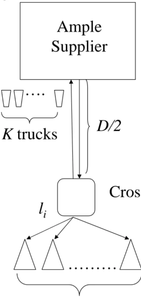
Figure 2.1: Illustration of the environment
Ample
Supplier
………
N retailers
l
iD/2
Cross-dock
….
K trucks
backordered. Retailers are supplied from an ample supplier via a fleet of K iden-tical trucks of capacity C that are used in the transportation of retailer orders. When a truck is available, units are carried from the ample supplier to a cross-dock station, which takes D/2 time units. The truck returns back to its base at the ample supplier after unloading at the cross-dock station. At the cross-dock station, items destined to each retailer are transferred to smaller sized vehicles to be conveyed to the retailers. We do not allow for any re-allocation of items to the retailers at the cross-dock station. We assume that the transportation is not capacitated after the cross-dock point. The lead time between retailers and the cross-dock point, which we refer as minor lead time, is li for retailer i.
Therefore, the order delivery lead time for retailer i is Li, where Li = li+ D/2.
Figure 2.1 illustrates the considered system. Holding cost per unit per time is charged at each retailer with rate hi. There is a common fixed order setup cost
for each order, which is linear to the truck capacity, A(C) = a × C for a > 0. The shortage cost per unit per time at retailer i is incurred at a rate of βi. Any
possible additional costs for monitoring the inventory system continuously are ignored. The joint orders are satisfied based on the first come-first serve (FCFS) rule at the ample supplier. Under this policy and cost structure, the objective is to minimize the expected total cost per unit time.
Due to the ordering cost structure, retailers implement a joint replenishment policy to manage their inventory and replenishment decisions. Since we are con-sidering an ample supplier, the orders received from the retailers constitute a compound renewal process, where inter-order time, Y , and the order quantity,
Q0, have a joint density, fY,Q0(y, q). Joint orders received by the ample supplier
are shipped immediately by trucks if there are sufficiently many trucks available to hold the existing order. In such a case, any given loaded truck spends a total of D time units to reach to the cross-dock point, unload the item and return back to its base. If there are not sufficiently many trucks available at the time of an order trigger at the base, then the order waits until enough number of trucks become available. Hence, the shipment operations of the retailer orders at the ample supplier can be modeled as a queueing model where the orders are the
customers in the system and the trucks are the servers which are busy while
carrying the materials to the cross-dock point and return back.
We assume that the retailers use (Q, S) policy of Renberg and Planche [30] as the joint replenishment policy for controlling their inventory in this study. In this continuous review policy, whenever a total demand of Q units are accumu-lated at the retailer level, a joint order of size Q is given to the supplier, and the inventory positions of the retailers are raised to the vector of order-up-to levels S=(S1, S2, ..., SN). We ignore the truck loading and unloading times,
how-ever they could be easily incorporated to our model by modifying the existing parameters.
2.2
Preliminary Analysis
In this section we present the methods that we use in our analysis. First, we introduce our notation. Let ri be the probability that the demand is for retailer
i, given that a demand arrival has occurred. Since demand process is Poisson, we
have ri = λi/λ0, where λ0 = ΣNi=1λi. Under the (Q, S) policy, a cycle is defined
as the time between two consecutive joint order placements, where the inventory positions of all retailers are raised to S = (S1, S2, ..., SN). Inter-order time, which
is denoted by X is the cycle length. Since the last epoch, total of Q retailer demands must be accumulated to place an order again. Hence, fX,Q0(x, q) = 0 for q 6= Q, which means that Q0is always equal to Q, where f denote the joint density
of X and Q0. Since the inter-arrival times of the demands are exponential, X has
an Erlang Q distribution with scale parameter λ0. Let F (x, k, λ) and f (x, k, λ)
denote the probability distribution and density functions of an Erlang random variable with shape and scale parameters k and λ, respectively and F (·)= 1−F (·) is the complementary distribution for any distribution function. For clarity and later use, we have the following definitions. At any given time t, IPi(t) denotes
the inventory position at retailer i and IP (t) denotes the total inventory position at the retailer level. IP (t) = ΣN
i=1IPi(t) ≤ ΣNi=1Si = S0. Also, let NIi(t) denote
the net inventory level at retailer i, and NI(t) = ΣN
i=1NIi(t) denote the total
inventory level at any given time t. A joint order is placed by the retailers when
IP (t) falls to S0− Q. If there are enough trucks on hand to meet the joint order
that is placed at time t, the order is immediately dispatched, otherwise it waits until a truck becomes available.
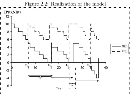
A typical realization is depicted in Figure 2.2. In this particular realization we ignore minor lead times li, and assume there are K = 2 trucks, S0 = 10,
C = 8 and Q = 5. Figure 2.2a shows the total inventory position IP (t) and
net inventory NI(t) at the retailer level and Figure 2.2b shows the number of available trucks on hand. First joint order occurs at t1, and it is dispatched
immediately since there are enough trucks available. Second order occurs at t2,
and it is dispatched without any delay, too. However the third joint order placed at time t3 is not dispatched immediately, since there is no available truck at
Figure 2.2: Realization of the model -6 -4 -2 0 2 4 6 8 10 12 0 10 20 30 40 Time NI(t) IP(t) -2 -1 0 1 2 3 0 10 20 30 40 Time Truck Level IP(t),NI(t) Truck Level D D/2 (a) (b) t3 t1 t2 t4 w t1 t2 t3 w
time t3. After the placement of the third joint order, number of trucks on hand
decreases from 0 to −1. When the number of trucks on hand is negative, there is at least one order that is waiting for a truck to be dispatched. The third joint order in this illustration is dispatched at t1 + D = t3+ w, when a truck returns
back to the ample supplier.
Let W denote the time a joint order waits for dispatching. In our particular realization, W = 0 for the first and the second joint orders, and W = w for the third one. The lead-time (total transit time) for retailer i, (Li), with the
is denoted by Li = Li+ W . W is a random variable and its distribution function
is denoted by FW(w) for w ≥ 0.
As mentioned above, joint orders are received from the retailers with an
Erlang − Q distributed inter-arrival time with scale parameter λ0 in a (Q, S)
policy. If Q ∈ (C/2, C] and there is an order integrity constraint, each joint order occupies exactly one truck. Hence, dispatching operations act as an EQ/D/K
queue when more than a 50% truck utilization is guaranteed. Enforcing a min-imum truck utilization may result in suboptimal policy parameters, however it is a common practice in industry due to the transportation limitations and high order set-up costs. Hence, FW(w), which is essential for deriving the operating
characteristics of our system, is identical to the waiting time distribution of an
EQ/D/K queue.
2.3
Derivation of the Operating Characteristics
In this section, the operating characteristics of our system are derived, and these expressions are used in calculating the total cost rate. Total cost of the system consists of two parts. The first part is the order setup cost and the latter is the holding and backorder costs. We begin with expected cycle length, E[X]. As noted in Section 2.2, X has an Erlang Q distribution with scale parameter λ0.
Therefore, expected cycle length is simply Q/λ0. In each cycle, the fixed ordering
cost of a joint retailer order is incurred once, and order setup cost rate is simply
A(C) × λ0/Q. The evaluation of the expected costs under the (Q, S) policy with
capacitated trucks and unlimited fleet size is analyzed by Cachon [10]. Note that
W = 0 and the lead-times (L1, L2, ..., LN) of the system are constants if there is
no limit on the fleet size. On the contrary, when the fleet size is limited, effective lead-times, Li = Li+ W , are random variables which may take any value on the
interval [Li, ∞).
Axsater [3] presents an approach, which can be used to evaluate the expected holding and backorder cost rate of a two-echelon inventory system consisting of
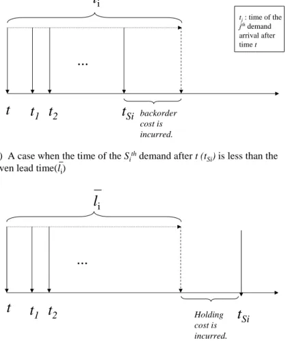
Figure 2.3: Illustrations of how backordering and holding costs per unit are in-curred
...
t
1t
2t
Si backorder cost is incurred....
t
1t
2t
Si Holding cost is incurred.j
j
t
t
tj: time of the jthdemand arrival after time tl
il
i(a) A case when the time of the Sithdemand after t (t
Si) is less than the
given lead time(li)
(b) A case when the time of the Sithdemand after t (t
Si) is greater than the
given lead time(li)
a single depot and multiple retailers, both following base-stock policies with base stock levels Si and deterministic lead-times. This approach is based on the
obser-vation that in such distribution systems, a unit ordered by retailer i is used to fill the Sth
i subsequent demand following this order. Accordingly, expected time for a
unit that is held in the inventory and the expected time a unit is backordered can be evaluated by relating the arrival time of the order and the arrival time of the
Sth
i subsequent demand. The illustrations of how the backordering and holding
costs are incurred for a unit are given in Figure 2.3a and Figure 2.3b, respectively. The unit demand that occurs at time t arrives after the Sth
i subsequent demand
the contrary, the unit demand that occurs at time t arrives before its Sth
i
subse-quent demand in Figure 2.3b. and holding cost per time is incurred for that unit. Cachon [10] adopts this approach to a similar environment, where the retailers use the (Q, S) policy in a coordinated fashion; there is an ample supplier, and an unlimited number of capacitated trucks are used for the distribution of items from the supplier to the retailers. We also use the same approach in our analysis. We first define the function gi(Si, li), which corresponds to the expected
hold-ing and backorder costs incurred per time per unit for retailer i with a base-stock level Si and a given effective lead time Li = Li+W = li, which is constant. Then,
gi(Si, li) = βi Z li 0 (li− x)f (x, Si, λi)dx + hi Z ∞ li (x − li)f (x, Si, λi)dx. (2.1)
The expected backorder time a unit would face is expressed by the first integral above, whereas the expected time a unit is stored in the inventory is expressed by the second one. From the properties of the gamma distribution, we can rewrite:
Z li 0 xf (x, Si, λi)dx = Si/λi Z li 0 f (x, Si+ 1, λi)dx (2.2)
which corresponds to the probability that Sth
i demand occurs before li. The
probability of this event is identical to the probability that Si or more demands
occur in [0, li]. Therefore we can write
Z li
0
f (x, Si, λi)dx = (1 − FP(Si− 1, λili)) (2.3)
where FP(y, λli) denotes the cumulative probability distribution of a Poisson
process with rate λ. Hence, we can rewrite Equation (2.1) as follows:
gi(Si, li) = 1 λi £ Si(hi+ βi)FP(Si, λili) − λili(hi+ βi)FP(Si− 1, λili) + βi(λili− Si) ¤ . (2.4) Equation (2.4) gives the expected holding and backorder costs a unit demand from retailer i faces when that unit demand triggers a joint replenishment de-cision. When Q = 1 in a (Q, S) policy, a unit demand always triggers a joint replenishment decision. Now we consider the general case when a unit demand to retailer i is arrived, but a joint replenishment decision is not triggered until a
total of Q ≥ 1 demands are accumulated. Let a unit demand to retailer i occurs at time τ , and the trigger of a joint replenishment decision that contains this unit demand to retailer i is delayed until τ + t. That joint order arrives at the retailer at τ + t + li. Let Mi denote the total number of the demands occur at retailer
i between τ and τ + t. When Mi = mi, the unit demand occured at τ is used
to fill the (Si − mi)th subsequent demand after τ + t. Therefore, the expected
holding and backorder cost that we incur for a unit demand from retailer i is simply gi(Si− mi, li). It must be noted that, when mi ≥ Si, gi(Si − mi, li) still
gives the expected holding and backorder cost that is incurred for a unit demand from retailer i. However, Equation (2.4) should be used for the calculation. The reader is referred to Axs¨ater [4] for a detailed proof.
Let M0 ≥ Mi be the total number of retailer demands (including i) that have
occurred in (τ, τ + t]. When M0 = n, the probability that mi of these n demands
are from retailer i is the probability of having mi successful draws out of n, where
ri = λi/λ0 is the probability of success. Let Z(mi|n) be the probability mass
function of the number of successful ones from n draws. Then,
Z(mi|n) = P r(Mi = mi|M0 = n) = (nmi)(ri)
mi(1 − r
i)n−mi.
It is known that M0 is a uniformly distributed integer on the interval [0, Q − 1]
(see Axs¨ater [4]). Finally, we can derive the expected holding and backorder cost per time per unit demanded from retailer i for a given effective lead-time Li = li
as below: 1 Q Q−1X n=0 n X mi=0 Z(mi|n)gi(Si− mi, li). (2.5)
After the expected holding and backorder cost rate for retailer i is analyzed for a given effective lead-time, we need the distribution function of the effective lead-time in order to calculate the expectation of the holding and backorder cost rate over effective lead-time. Since Li is constant, the distribution function of
the effective lead-time, Li = Li + W is determined by the distribution function
2.3.1
Derivation of the Waiting Time Distribution of an
Order for a Truck
In this subsection, we derive FW(w), which is essential for analyzing the operating
characteristics of our system. As mentioned in Section 2.2, the dispatching of the orders via trucks operates as a queueing system and FW(w) is identical to the
waiting time distribution of this EQ/D/K queue. The following theorem provides
a basis for the method that we use to derive FW(w).
Theorem 1 (Tijms [40], p.321): The waiting time distribution FW(w) in the
multi-server GI/D/c queue is the same as in the single-server GIc∗/D/1 queue
in which the inter-arrival time is distributed as the sum of c inter-arrival times in the GI/D/c queue.
The theorem has the following important corollary.
Corollary 1 (Tijms [40], p.321): The waiting time distribution (FW(w)) in the
Ek/D/c queue is identical to the waiting time distribution in the M/D/ck queue
with the same server utilization.
The dispatching of the trucks operate as an EQ/D/K queue. Due to the
Corrol-lary 1, in order to find the distribution of the time an order waits for dispatching, we need the waiting time distribution of an M/D/c queue where c = Q × K. We use the solution method that Franx [19] proposes to find FW(w) in an efficient
manner for such queues. In order to be coherent with the terminology, we use
customer and server instead of joint order and truck, respectively, from now on.
First, let pi(t) denote the probability of the system holding i customers at
time t. Since the service time is deterministic, all the customers in the service will have left the system at time t + D. Consequently, customers in the system at time t + D either have arrived during the time interval (t, t + D] or they were waiting for service at time t. Therefore the following expression can be written
by conditioning on the number of customers present at time t: pi(t + D) = Σcj=0pj(t) (λ0D)i i! e −λ0D + Σi+c j=c+1pj(t) (λ0D)i+c−j (i + c − j)!e −λ0D, t ∈ R, i ∈ N . (2.6) When there are less than c customers in the system at time t, all customers present at time t will be served at time t + D. If i customers arrive between t and
t + D then the number of customers at time t + D will be i. However, when there
are j > c customers in the system at time t, c of the customers will be served by time t + D. If there are i ≥ 0 customers in the system at t + D, then j − c + i customers must have arrived between t and t + D.
As t → ∞, we can obtain the stationary state probability of the number of customers in the system, which is denoted by pi = limt→∞pi(t) as
pi = Σcj=0pj (λ0D)i i! e −λ0D + Σi+c j=c+1pj (λ0D)i+c−j (i + c − j)!e −λ0D, i ∈ N . (2.7)
These expressions of pi’s constitute an infinite system of linear equations with
the normalization equationP∞i=0pi = 1. This infinite system of linear equations
can be reduced to a finite system of linear equations by the following theorem: Theorem 2 (Tijms [40],p.289): The state probabilities (pj) of the M/D/c queue
exhibit geometric tail property:
pj ≈ δγ−j
for large j, where γ ∈ (1, ∞) is the unique solution of the equation: λ0D(1 − γ) + c ln(γ) = 0.
Also, the constant δ is given by
δ = (c − λ0Dγ)−1
c−1
X
i=0
pi(γi− γc).
Via this geometric tail property, the infinite system of linear equations for the
pj’s is reduced to a finite system by replacing pj by pM(1/γ)j−M for j > M and
methods in the literature, which can be used to solve finite systems of linear equations. The computational complexity of this method is O(M3)
We apply an iterative method for choosing the appropriate M with a predeter-mined error bound, ². The algorithm of the iterative method is demonstrated in the Appendix A. 1. After deriving stationary state probabilities pi, we can derive
the stationary probability qi of the queue containing i customers, by q0 = Σc0pi
and qi = pi+c for i > 0. Also we define the cumulative probability that there are
j or less customers in the queue as Gj =
Pj
i=0qi. Finally, the following theorem
provides an expression for the Waiting Time Distribution in the queue. Theorem 3 (Franx, [19]): For a M/D/c queue,
FW(w) = e−λ0(awD−w) aXwc−1 j=0 Gawc−j−1 λj0(awD − w)j j!
where aw is the greatest integer less than or equal to the Dw + 1 for w ≥ 0.
A critical point for our analysis is whether this random structure of the effective lead-time Li permits order-crossing or not, because in the stochastic lead time
environments, order crossing considerably complicates the situation. Considering that the time a unit-demand is held in the inventory (or backordered) is calculated based on the observation that a unit-demand from retailer i is used to fill the
Sth
i subsequent demand, no order crossing is the sine qua non condition of the
approach that is employed by Axs¨ater [3]. Since the joint orders are served based on the FCFS rule and the service times are deterministic, the no-order-crossing condition is satisfied at all times, which enables us to use the approach employed by Axs¨ater [3] in our system.
2.3.2
Objective Function
After the analysis for a given effective lead-time and the derivation of the distri-bution FW(w) of the waiting time W for truck that a joint order encounters, we
take the expectation of the holding and backlogging costs over effective lead-times for each retailer i.
The waiting time of an order before dispatching is a mixed distribution. Let
C and D denote the sets, where FW(w) is continuous and discrete respectively.
Recall that FW(w) is dependent on K, because the number of servers is c = K ×Q
in Theorem 3. By taking the expectation of the cost expression in Equation (2.5) with respect to W , we can derive the expected unit holding and backorder cost of retailer i as below: U(Q, S, K)i = Z w∈C 1 Q Q−1 X n=0 n X mi=0 Z(mi|n)gi(Si− mi, Li+ w)dFW(w)+ X w∈D 1 Q Q−1 X n=0 n X mi=0 Z(mi|n)gi(Si− mi, Li+ w)P (Wq = w) (2.8)
Finally, the expected cost rate of the the whole system is given by:
AC(Q, S, K, C) = λ0 A(C) Q + N X i=1 λiU(Q, S, K)i. (2.9)
The first part of the equation above represents the order setup cost rate and the second part represents the expected holding and backorder costs incurred per unit time of our distribution system that is using a (Q, S) policy with a fleet of K trucks, each having a capacity of C. Considering the truck utilization constraint, the optimization problem of our system can be stated as follows:
Min AC(Q, S, K, C) s.t. Q ∈ (C/2, C].
2.4
Analysis of the Total Cost Rate Function
In this section, some characteristics of the function AC(Q, S, K, C) and the rela-tions between the decision variables are discussed. We use these relarela-tions in our search algorithms that are constructed for different problem scenarios.
Axs¨ater [4] demonstrates that the unit holding and backorder cost rate func-tion, which is given in Equation (2.5), is convex in Si for each retailer. Recall
that the U(Q, S, K)i is the expectation of the unit holding and backorder cost
rate function over effective lead-times. Since expectation is a linear operator,
U(Q, S, K)i is also convex in Si. Therefore, the optimal order-up-to levels for
each retailer i (S∗
i(Q, K)) for a given joint-order quantity Q and a fleet size K
can easily be found. Let S∗(Q, K) = (S∗
1(Q, K), S2∗(Q, K), ..., SN∗(Q, K)). When
the number of the fleet size and the capacity of the trucks are given, the total cost rate function AC(Q, S∗(Q, K), K, C) is not necessarily convex in Q. Therefore
we need to search over the feasible interval (C/2, C] to find the optimal shipment quantity Q∗ for given K and C. Next, we analyze the effects of K on the total
cost rate of our distribution system.
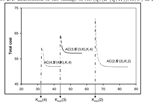
It is important to note that the total cost rate of the system goes to infinity if the M/D/KQ queue blows up. Hence, there is a minimum number of trucks, say Kmin(Q), that will guarantee that the queueing system operates at the steady
state in the long run for a given Q value. Kmin(Q) is the smallest positive integer
K that satisfies ρ = (λ0× D/K × Q) < 1.
Also as K increases, the system begins to behave as if there is no transporta-tion limitatransporta-tion. In our numerical results, we observe that each truck added to
Kmin(Q) brings a lower decrease in the total cost rate. Although this observation
is parallel to that of Rolfe [31], who shows that the average waiting time in the queue is a convex decreasing function of the number of servers, we could not prove it analytically in our problem due to the intricacy of the expressions in our problem.
demonstrated in Figure 2.4 for Q = 2, 3, 4 when λ0 = 16, D = 8, N = 16,
A(C) = C, h = 1 and βi = 2 for all retailers.
Figure 2.4: Illustration of the change of AC(Q, (S∗(Q, K)), K, C) in K
45 55 65 75 20 30 40 50 60 70 80 90 T o ta l c o s t AC(3,S*(3,K),K,4) AC(4,S*(4,K),K,4) AC(2,S*(2),K,2)
Kmin(4) Kmin(3) Kmin(2)
K (Fleet Size)
Recall that the trucks of the system operate as an EQ/D/K queue while the
system uses a (Q, S) policy and posseses K trucks. Also, recall that the wait-ing time distributions of EQ/D/K queues and M/D/KQ queues are identical.
Therefore, in a system that uses (Q, S) policy for a given fleet size K, when one more truck is purchased, the waiting time distribution for a truck F (w) is the waiting time distribution of a M/D/(K + 1)Q queue. So, buying one more truck changes the waiting time distribution of the system as if we buy Q more servers to a M/D/KQ queue. On the other hand if the system used (Q0, S) policy for
Q0 > Q, buying one more truck would change the distribution of the system as
if we bought Q0 more servers to a M/D/KQ0 queue. Therefore, the traffic rate ρ
of the system decreases more slowly with K, when the system uses (Q, S) policy for Q0 > Q.
Let AC(Q, (S∗(Q)), C) denote the average total cost rate function, when there
dispatched with trucks of capacity C. In parallel to the discussion above, we ob-serve in our numerical results that AC(Q0, (S∗(Q0, K)), K, C) approaches quicker
to AC(Q0, (S∗(Q0)), C) as K increases compared to AC(Q, (S∗(Q, K)), K, C)
ap-proaches to AC(Q, (S∗(Q)), C) when Q < Q0.
Note that Kmin(4) < Kmin(3) < Kmin(2) in Figure 2.4. Since Kmin(Q) is
the minimum integer value of K that makes ρ = (λ0D/KQ) < 1, Kmin(.) is a
non-increasing function of Q. Next, we analyze the effects of Q and C on the total cost rate for a given fleet size K.
We now define Qmin(K), which is the minimum joint order size to carry on
a (Q, S) policy for a given fleet size K. Qmin(K) is the smallest positive integer
Q that satisfies ρ = (λ0 × D/K × Q) < 1. We also note that Qmin(K) is
non-increasing in K, that is Qmin(K) ≤ Qmin(K0) if K0 < K. Figure 2.5 sketches
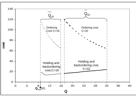
the effects of Q over the total cost rates for a given K = 2 and when we have two truck capacity options C = 16 and C = 32 with λ0 = 16, D = 1, N = 4,
A(C) = 4 × C, h = 1 and βi = 4. When there is no fleet size limitation, the
Figure 2.5: Illustration of the change of AC(Q, (S∗(Q, K)), K, C) in Q for a given
K 0 20 40 60 80 100 120 140 0 4 8 12 16 20 24 28 32 36 40 c o s t Ordering Cost C=16 Ordering cost C=32 Holding and backordering cost,C=16 Holding and backordering cost, C=32 Qmin(K) Q16 Q32 Q
holding and backorder cost rates increase as Q increases in (Q, S) policy. However, as we can observe from Figure 2.5, the holding and backorder cost rate faces a decrease, while we increase Q at the beginning. This decline in the holding and
backorder costs is due to the decrease in the traffic ratio of the M/D/KQ queue. In general, we notice a decrease in the holding and backorder cost rate at the beginning when the traffic ratio λ0×D
K×Qmin(K) is greater than 0.8 in our numerical results. An increase in Q leads to a decrease in the traffic ratio, which leads to a decrease in the holding and backorder cost rate when the traffic ratio is high. In other words, the effect of decreasing the traffic ratio on holding and backorder costs is more dominant than the effect of increasing the joint order quantity when the traffic ratio is high.
Here we observe from Figure 2.5 that the order setup cost decreases as Q increases for a given C, since the order setup cost is A(C) × λ0/Q and A(C)
is a linear function of C. The order setup cost rates are the same for different truck capacities as long as they are utilized with 100% utilization. Let QC = (C1, C2, ..., Cm), with C1 < C2 < ... < Cm denote the possible values of the
order quantities for a given C. The following proposition suggests that using trucks with a higher utilization is always more profitable without changing other decision variables whenever it is possible.
Proposition 1: Suppose C < C0. If the intersection of Q
C and QC0 is non-empty, it is always more profitable to choose C as a truck capacity for the intersecting Q values.
Proof: Referring to Subsection 2.3.2, AC(Q, S, K, C) consists of two parts: the order setup cost rate, which is λ0× A(C)Q , and the holding and backordering
cost rates, which do not change with C when the other parameters are the same. So for C < C0, if there is a Q such that Q ∈ Q
C and Q ∈ QC0, then the holding and backorder cost rates of C and C0 are the same. However,
λ0× A(C)Q < λ0× A(C
0)
Q since A(C) < A(C0).¤
2.5
Different Scenarios and Solution Procedures
Firms can face the problem of transportation limitation in different forms. For instance the firm may not have the chance to choose the capacity if there is solely
one kind of truck. In this section, we list different transportation scenarios that firms can encounter. In each of these scenarios, firms have to make decisions about the parameters of the joint order policy and about the features of their means of transportation. In order to help this decision-making process of the managers, we develop solution procedures based on the results that we discuss in Section 2.4. In this section, we take a new cost parameter into account: φ(C), which is the depreciation and maintenance cost rate per time we incur to a truck with a capacity C. We assume that φ(C) is a linear function of C, and our solution procedures are based upon this assumption.
Single Truck Capacity Option
This case can be frequently encountered in the industry. For instance, suppose that the truck to be used in the transportation is very specific to the unit sold in the retailers and that’s why it is not vended often in the market and product diversity does not exist for that truck of interest (e.g. hazardous materials). In this case, K, Q and S∗(Q, K) are jointly optimised for a given truck capacity option C. Hence, built on our discussions in Section 2.4, Search Algorithm 1, given in Appendix A.2 is suggested.
Several Truck Capacity Options
This type of limitation is the most common type that the firms encounter in the market. Suppose that there are many truck producers, and they are providing trucks of different capacities. Therefore, there is a capacity option set, C = (C1, C2, ..., Cm), which consists of m truck capacity options (C1 < C2 < ... < Cm)
that a firm can choose. Besides the fleet size K, order quantity Q and order-up to levels S∗(Q, K), the firms also have to decide upon the truck capacity C in order
to minimize their total cost rates. Therefore, we suggest the Search Algorithm 2, given in Appendix A.2.
Since the single truck capacity option scenario is a special case of the several truck capacity options scenario, we only mention about Search Algorithm 2 in this section. In this search algorithm, we first obtain the possible values of the order quantities QCi for each Ci ∈ C. Due to the Proposition 1, we delete the
Ci ∈ C, we find the minimum number of the trucks needed Kmin(Q) as well as
the critical number of the fleet size, Kmax(Q, φ(Ci)) that is given by Equation
(A.2), where buying one more truck increases the total cost rate (in the presence of maintenance/depreciation cost rate) for the first time for every Q ∈ QCi. Since the truck/maintenance cost is assumed to be linear with K, Kmax(Q, φ(Ci))
would give the optimal fleet size K∗ for a given joint order quantity Q if the
conjecture on the convex decreasing behavior of the AC(Q, S∗(K, Q), K, C
i) holds
true. Subsequently, we search for the best joint order quantity Q∗
i for a given
capacity Ci first, and then we choose the capacity C∗ that brings the minimum
cost rate among all of the capacity options. Hence, this algorithm finds K∗, C∗,
Q∗ and S∗(K∗, Q∗) accordingly.
Next, we consider the case, where the firm decides on the capacity of the trucks for a given number of the fleet size. The motivation behind a given fleet size number can be the area restriction of the hangar as well as the investment constraints. First, suppose that the truck producer guarantees to provide trucks with the capacity that the firm demands. Since the order setup cost rate is A(C)×
λ0/Q, the firm aims to use the trucks with 100% utilization. In other words, the
firm would like to purchase the trucks with capacity C = Q. In addition, we consider that the truck producer firm can have an upper limit for the capacity of the trucks, and no trucks with a capacity more than Cmax can be produced.
The firm has to revise the fleet size (K) decision, if Qmin(K) > Cmax. Otherwise,
the firm has to decide upon the joint order quantity Q∗ ∈ [Q
min(K), Cmax] and
the order-up to levels S∗(Q∗, K), for a given fleet size K in order to minimize
the total cost rate of the system. After deciding the order quantity Q∗, the firm
requires trucks with capacity C = Q∗ from the truck producer.
Now, rather than full flexibility on the capacity, we consider the case when there is a capacity option set, C = (C1, C2, ..., Cm), with (C1 < C2 < ... < Cm).
Suppose that the fleet size is K. Similar to the previous setting, the firm has to revise the fleet size (K) decision, when Qmin(K) > Cm. We suggest the Search
2.6
Numerical Study
This section details a numerical study that illustrates the general behavior of the optimal policy parameters and the average cost rate with respect to different cost and system parameters. For the sensitivity analysis, all combinations of the following sets are analyzed: λ0={2, 4, 8, 16, 32}, D={1, 2, 8}, C={2, 4, 8, 16,
32}, a = A(C)/C={0.25, 1, 4}, hi={1}, βi={2, 4, 16, 32}, N={2, 4, 16}.
In all of the scenarios, the retailers are identical (same mean demand, holding and backorder cost rates and lead-times). Note that we ignore the truck mainte-nance and depreciation cost rate φ(C) as well as the minor lead times, li = 0, in
our numerical analysis part.
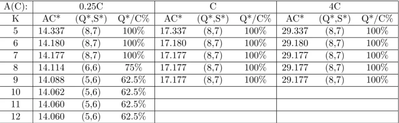
Table 2.1: The Effects of the Change in a = A(C)/C and K on Total Cost Rate
A(C): 0.25C C 4C
K AC* (Q*,S*) Q*/C% AC* (Q*,S*) Q*/C% AC* (Q*,S*) Q*/C%
5 14.337 (8,7) 100% 17.337 (8,7) 100% 29.337 (8,7) 100% 6 14.180 (8,7) 100% 17.180 (8,7) 100% 29.180 (8,7) 100% 7 14.177 (8,7) 100% 17.177 (8,7) 100% 29.177 (8,7) 100% 8 14.114 (6,6) 75% 17.177 (8,7) 100% 29.177 (8,7) 100% 9 14.088 (5,6) 62.5% 17.177 (8,7) 100% 29.177 (8,7) 100% 10 14.062 (5,6) 62.5% 11 14.060 (5,6) 62.5% 12 14.060 (5,6) 62.5%
The influence of A(C) and K on the performance of the system In Table 2.1, we tabulate how the average cost rate changes with A(C) = a × C and fleet size K, where N = 4, λ0 = 4, C = 8, βi = 4 for all i and D = 8. We
observe that for a given capacity C, truck utilization Q∗/C has a non-increasing
structure when the fleet size K increases, because the system is enforced to have a higher utilization when there is a scarcity of trucks. In addition, as a increases,
Q∗/C increases as well. This is due to the fact that the savings from the order
set-up costs dominate the increase in holding and backorder costs as A(C) increases. Hence, the truck utilization increases as A(C) increases. Also, note that S∗ has
a non-increasing behavior with the fleet size. We can assert that the retailers try to balance the delay due to the absence of enough trucks with higher order up-to
levels. Parallel to the conjecture that we made in Section 2.4, we observe the convex decreasing behavior of the total cost rate with K in Table 2.1 as well as in all of our numerical studies for the same system parameters.
The influence of backorder cost rate and K on the performance of the system
Table 2.2 illustrates the impacts of backorder cost rate βi and fleet size K on the
total cost rate where N = 4, λ0 = 4, C = 8, A(C) = C and D = 8.
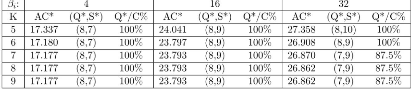
Table 2.2: The Effects of the Change in βi and K on Total Cost Rate
βi: 4 16 32
K AC* (Q*,S*) Q*/C% AC* (Q*,S*) Q*/C% AC* (Q*,S*) Q*/C%
5 17.337 (8,7) 100% 24.041 (8,9) 100% 27.358 (8,10) 100%
6 17.180 (8,7) 100% 23.797 (8,9) 100% 26.908 (8,9) 100%
7 17.177 (8,7) 100% 23.793 (8,9) 100% 26.870 (7,9) 87.5%
8 17.177 (8,7) 100% 23.793 (8,9) 100% 26.862 (7,9) 87.5%
9 17.177 (8,7) 100% 23.793 (8,9) 100% 26.862 (7,9) 87.5%
From the numerical results, we observe that the retailers respond to higher backorder cost rates by increasing their order up-to levels. Also, contrary to the Table 2.1, truck utilization is nonincreasing in βi, because the savings from the
holding and backorder costs begin to dominate the increase in order set-up costs while having a lower truck utilization as βi increases.
Joint Effects of K and C
Suppose that the truck capacity is exogenous to our system. In such a case, C has a great influence over the performance of our system, since it sets the limits for
Q. Note that the order set-up cost rate is identical for all C as long as the trucks
are utilized 100%, since A(C)×λ0
Q = a × λ0 when Q = C. Next, we present Table
2.3, which depicts the effects of C and K jointly on total cost rate where N = 4,
λ0 = 2, βi = 8, A(C) = C and D = 8. As expected, truck utilization percentage
100×Q∗
C decreases whereas order up-to levels increase for bigger C. Notice that
in some of the cases in Table 2.3, there can be an insignificant decrease in cost rates with respect to K. This is due to the fact that in these cases the traffic rate
ρ = λ0D
KQ is not that much high for the smallest K that makes ρ < 1. In addition,
quickly to its lower bound for bigger C. Recall that the lower bound of AC is the cost rate of a system with the same parameters, where there is no limitation at all on the fleet size. If truck maintenance and depreciation cost rate φ(C) is taken into consideration, Kφ(C) must be added to each of the cost rates given in Table 2.3 and the decisions must be made accordingly.
Table 2.3: The Effects of C and K on Total Cost Rate for C = 2, 4, 8, 16 and 32
C=2 C=4 K AC* (Q*,S*) Q*/C% K AC* (Q*,S*) Q*/C% 9 13.246 (2,4) 100% 5 11.682 (4,4) 100% 10 11.494 (2,3) 100% 6 11.330 (4,4) 100% 11 10.897 (2,3) 100% 7 11.309 (4,4) 100% 12 10.735 (2,3) 100% 8 11.307 (4,4) 100% 13 10.687 (2,3) 100% 9 11.307 (4,4) 100% 14 10.674 (2,3) 100% 15 10.670 (2,3) 100% 16 10.669 (2,3) 100% 17 10.669 (2,3) 100% C=8 C=16 K AC* (Q*,S*) Q*/C% K AC* (Q*,S*) Q*/C% 3 12.332 (8,4) 100% 2 14.212 (12,5) 75% 4 12.182 (7,4) 87.50% 3 14.147 (11,5) 68.75% 5 12.179 (7,4) 87.50% 4 14.147 (11,5) 68.75% 6 12.179 (7,4) 87.50% 5 14.147 (11,5) 68.75% C=32 K AC* (Q*,S*) Q*/C% 1 18.129 (21,7) 65.63% 2 17.095 (17,6) 53.13% 3 17.095 (17,6) 53.13% Effects of D/2 and λ0
The impacts of the distance between the ample supplier and the cross-dock point
D/2 on total cost rate AC are similar to those of the total demand rate λ0.
Both D and λ0 increase the traffic ratio ρ as well as the expected demand during
lead-time. Hence, the system’s reactions to higher D and λ0 are higher order
up-to levels at the retailer level and a bigger fleet size. Note that only holding and backorder costs at the retailer level increase as D increases, whereas order setup, holding and backorder costs increase as λ0 increases for the same Q. In
our numerical results, we observe that truck utilization Q∗/C increases with both
D and λ0. Our observations are consistent with Cachon’s [10] suggestions, which
claim that Q∗is increasing in both lead-time L and λ
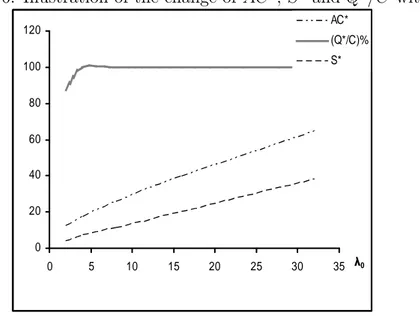
0. Figure 2.6 depicts how the
total cost rate AC∗, order up-to level S∗ and truck utilization percentage Q∗/C
change with λ0 where C = 8, A(C) = C, βi = 4, N = 4 and D = 8 provided that
there is an ample number of trucks.
Figure 2.6: Illustration of the change of AC∗, S∗ and Q∗/C with λ
0 0 20 40 60 80 100 120 0 5 10 15 20 25 30 35 0 AC* (Q*/C)% S*
Effects of the number of retailers N
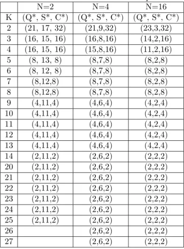
Table 2.4 tabulates how the optimal system parameters (Q∗, S∗, C∗) change with
K for different N, where we have a capacity option set C = 2, 4, 8, 16, 32, λ0 = 4,
βi = 4, A(C) = C and D = 8. In our numerical results, we observe an increase
in holding and backordering costs as N increases. This increase is due to the fact that we enjoy the benefits of risk pooling when N is smaller. Note that the total demand rate λ0 is remained fixed for all N. When N is greater, a bigger
amount of inventory is held at the retailer level for the same λ0. When there is no
fleet size limitation, we expect that an increase in N lead to a decrease in truck utilization percentage (See Cachon [10]). However, we observe that (Q∗/C)%
increases as N increases when K = 2 in Table 2.4. In this specific case, limited fleet size brings about a longer effective lead time, which increases Q∗/C%, and