MASTER PRODUCTION SCHEDULING
UNDER UNCERTAINTY WITH
CONTROLLABLE PROCESSING TIMES
a thesis
submitted to the department of industrial engineering
and the institute of engineering and science
of bilkent university
in partial fulfillment of the requirements
for the degree of
master of science
By
Ersin K¨
orpeo˘
glu
July, 2009
I certify that I have read this thesis and that in my opinion it is fully adequate, in scope and in quality, as a thesis for the degree of Master of Science.
Prof. Dr. M. Selim Akt¨urk (Supervisor)
I certify that I have read this thesis and that in my opinion it is fully adequate, in scope and in quality, as a thesis for the degree of Master of Science.
Assoc. Prof. Dr. Hande Yaman
I certify that I have read this thesis and that in my opinion it is fully adequate, in scope and in quality, as a thesis for the degree of Master of Science.
Asst. Prof. Dr. Ay¸seg¨ul Altın
Approved for the Institute of Engineering and Science:
Prof. Dr. Mehmet B. Baray
Director of the Institute Engineering and Science
ABSTRACT
MASTER PRODUCTION SCHEDULING UNDER
UNCERTAINTY WITH CONTROLLABLE
PROCESSING TIMES
Ersin K¨orpeo˘glu
M.S. in Industrial Engineering Supervisor: Prof. Dr. M. Selim Akt¨urk
July, 2009
Master Production Schedules (MPS) are widely used in industry especially within Enterprise Resource Planning (ERP) Software. MPS assumes infinite capacity, fixed processing times and a single scenario for demand forecasts. In this thesis, we questioned these assumptions and considered a problem with finite capacity, controllable processing times and finally and most importantly, several demand scenarios instead of just one. We used a multi-stage stochastic programming ap-proach in order to come up with maximum expected profit given the demand scenarios. We used controllable processing times, which are feasible in most of the scheduling practice in industry, to achieve a flexibility in capacity usage. We provided a non-linear mixed integer programming formulation for our problem. Afterwards, we analyzed two sub-problems to simplify the structure of the objec-tive function and suggested alternaobjec-tive linearizations. We considered easier cases of our problem, proposed sufficient conditions for optimality and established the computational complexity status for two special cases. We conducted three ex-periments, to test computational performance of the formulations, to analyze the profit performance of the multi-stage solutions and finally, to analyze the effect of controllability on profit. Our computational studies show that one of the proposed formulations solves large instances in a very small amount of time. The second experiment suggests that the performance of multi-stage solutions is significantly better than the one of solutions obtained using single scenario strategies in terms of relative regret. Finally, the third experiment shows that controllability significantly increases the performance of multi-stage solutions.
Keywords: Master Production Scheduling, Multi-stage stochastic programming, Controllable processing times.
¨
OZET
BEL˙IRS˙IZL˙IK ALTINDA KONTROL ED˙ILEB˙IL˙IR
˙IS¸LEM S ¨
URELER˙IYLE TEMEL ¨
URET˙IM
C
¸ ˙IZELGELEMES˙I
Ersin K¨orpeo˘gluEnd¨ustri M¨uhendisli˘gi, Y¨uksek Lisans Tez Y¨oneticisi: Prof. Dr. M. Selim Akt¨urk
Temmuz, 2009
Ana ¨uretim ¸cizelgelemeleri (MPS) end¨ustride ¨ozellikle Kurumsal Kaynak Plan-laması (ERP) yazılımlarında sıklıkla kullanılmaktadır. MPS sınırsız kapasite, sabit i¸slem s¨ureleri ve tek senaryoya dayalı talep tahminleri varsayımında bu-lunmaktadır. Bu tezde, bu varsayımları sorguladık ve sınırlı kapasite, kon-trol edilebilir i¸slem s¨ureleri, son ve en ¨onemli olarak da bir yerine birden ¸cok senaryoya dayalı talep tahminlerini i¸ceren bir problemi ele aldık. C¸ e¸sitli talep senaryoları verildi˘ginde en y¨uksek beklenen kˆarı elde etmek amacıyla ¸cok a¸samalı olasılıksal programlama yakla¸sımı kullandık. Pek ¸cok end¨ustri uygulamasının olanak sa˘gladı˘gı kontrol edilebilir i¸slem s¨urelerini kapasite kullanımında esnek-lik sa˘glamak amacıyla kullandık. De˘gerlendirdi˘gimiz problem i¸cin do˘grusal ol-mayan karı¸sık tamsayılı programlama g¨osterimi ¨onerdik. Daha sonrasında iki tane alt problem inceleyerek hedef fonksiyonunun yapısını ortaya ¸cıkarttık ve ¨
onerdi˘gimiz ilk g¨osterim icin iki alternatif do˘grusalla¸stırma ¨onerdik. Ana prob-lemin daha basit hallerini inceleyerek, bazı yeterli ko¸sullar ortaya ¸cıkardık ve iki ¨
ozel durumun hesaplama karma¸sıklı˘gını g¨osterdik. ¨Onerdi˘gimiz modellerin zaman performansını, ¸cok a¸samalı olasılıksal programlama ¸c¨oz¨um performansını ve son olarak kontrol edilebilirli˘gin katkısını ¨ol¸ct¨u˘g¨um¨uz ¨u¸c tane deneysel ¸calı¸sma yaptık. Deneysel ¸calı¸smalar, ¨onerdi˘gimiz modellerden birinin b¨uy¨uk problem i¸cin bile ¸cok hızlı ¸calı¸stı˘gını, ¸cok a¸samalı olasılıksal programlama ¸c¨oz¨um performansının tekli senaryo stratejilerine oranla ¸cok daha iyi oldu˘gunu ve son olarak kontrol edilebilirli˘gin ¸cok a¸samalı olasılıksal programlama ¸c¨oz¨um performansını belirgin bir ¸sekilde y¨ukseltti˘gini g¨osterdi.
Anahtar s¨ozc¨ukler : Ana ¨uretim ¸cizelgelemesi, Kontrol edilebilir i¸slem s¨ureleri, C¸ ok a¸samalı olasılıksal programlama.
Dedicated to Gizem
Mustafa and G¨ulhayat ...
Acknowledgement
I would like to sincerely thank to my thesis supervisor and advisor Prof. M. Selim Akt¨urk for his precious and perpetual guidance and encouragement throughout this study and my M.S. studies. His unconditional belief in me, his patience and interest made this thesis possible.
I would also like to thank to Prof. Hande Yaman for kindly guiding me in preparation of this dissertation and giving me the upmost analytical support during my studies. I am also grateful for her patience while answering my endless questions and her time.
I gratefully acknowledge Prof. Ay¸seg¨ul Altın who have given her time to read this manuscript and offered valuable advice.
I am especially indebted to my fianc´ee Gizem for her love, encouragement and endless support which made this thesis possible. I can never thank her enough for being there for me anytime I needed. I also am grateful to my father Mustafa and mother G¨ulhayat for all the spiritual and financial support that they perpetually provided during and before my M.S. studies.
I would like to thank to T ¨UB˙ITAK for providing the financial support for my M.S. study.
Contents
1 Introduction 1
2 Problem Definition and Literature Review 4
2.1 Problem Description . . . 4 2.2 Controllable Processing Times . . . 5 2.3 Multi-stage Stochastic Programming . . . 6
2.3.1 Robust Optimization and Multi-stage Stochastic Program-ming . . . 7 2.3.2 Multi-stage Stochastic Model and Scenario Tree . . . 9 2.4 Master Production Scheduling and Available to Promise . . . 12
3 The Stochastic Model 14
3.1 The Multi-Stage Stochastic Programming Formulation . . . 14 3.2 Two Sub-problems . . . 17
3.2.1 The Single Period Capacitated Deterministic Scheduling Problem with Cost Minimization Objective . . . 17
CONTENTS viii
3.2.2 The Single Period Capacitated Deterministic Problem with
Profit Maximization Objective . . . 19
3.3 The Formulation with a Reduced Size . . . 23
3.4 An Alternative Linearization of the Stochastic Formulation (SF) . 23 4 On Easy Cases and Complexity 27 4.1 Sufficient Conditions for Optimality . . . 27
4.2 Stochastic Problem with no Postponement Cost . . . 29
4.3 The Deterministic Problem . . . 30
4.4 The Structure of Stochastic Formulation SF . . . 31
5 Computational Results 36 5.1 The Design of Experiments and the Environment Generated . . . 37
5.2 Tests on CPU Performance . . . 39
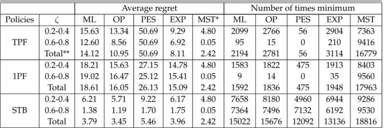
5.3 Experiments on Comparison of Multi-stage to Single Scenario Strategies . . . 41
5.3.1 T Period Frozen Policy . . . 47
5.3.2 One Period Frozen Myopic Adjustment Policy . . . 52
5.3.3 One Period Frozen Scenario Tree Based Demand Selection Policy . . . 58
5.3.4 Effects of Shortage and Excess Production . . . 64
5.4 Experiments on the Effect of Controllability . . . 68
CONTENTS ix
6 Conclusion 71
6.1 Summary . . . 71 6.2 Contribution . . . 72 6.3 Future Research Directions . . . 73
List of Figures
2.1 A Scenario Tree . . . 9
3.1 Profit charts in different cases . . . 22
4.1 A counter example for totally unimodularity of constraint matrix of SF . . . 32 4.2 A counter example for structure in Hemmecke et al. [19] . . . 34
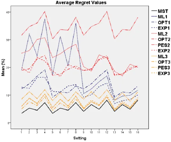
5.1 Average regrets of strategy policy combinations and multi-stage for combinations of factors C, D, F, and G. . . 47 5.2 Cross section of regret function as shortage factor is fixed. . . 66 5.3 Cross section of regret function as excess factor is fixed. . . 67 5.4 Cross section of regret function where shortage and excess are equal. 67
List of Tables
2.1 The profit of several strategies in different cases . . . 11 2.2 Relative regret of several strategies in different scenarios . . . 11
4.1 Constraint coefficient matrix for stochastic formulation of Figure 4.1 32 4.2 Constraint coefficient matrix for stochastic formulation of Figure 4.2 34
5.1 Experimental design factors and their settings. . . 38 5.2 Average, maximum, and number of times max values of each factor. 40 5.3 Factors used in the experiments. . . 45 5.4 Average relative regret and number of times minimum values of
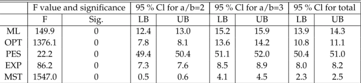
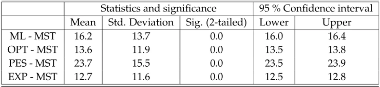
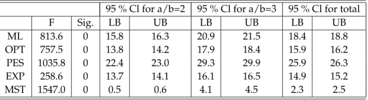
each scenario selection strategy. . . 45 5.5 Pairwise statistics of differences between regrets for all data. . . . 48 5.6 ANOVA table for compression cost exponent a/b. . . 48 5.7 Pairwise statistics of differences between regrets for cases where
a/b = 2 and a/b = 3. . . 49 5.8 ANOVA tables for capacity factor. . . 50
LIST OF TABLES xii
5.9 Pairwise statistics of differences between regrets for capacity factor 0.2 and 0.4. . . 51 5.10 Pairwise statistics of differences between regrets for capacity factor
0.6 and 0.8. . . 51 5.11 ANOVA tables for business factor. . . 52 5.12 Pairwise statistics of differences between regrets for [0,20] and
[0,40]. . . 52 5.13 Pairwise statistics of differences between regrets for [10,30]. . . 52 5.14 Pairwise statistics of differences between regrets for all data. . . . 53 5.15 ANOVA tables for compression cost exponent a/b. . . 54 5.16 Pairwise statistics of differences between regrets of strategies for
cases where a/b = 2 and a/b = 3. . . 55 5.17 ANOVA tables for capacity factor. . . 56 5.18 Pairwise statistics of differences between regrets for capacity factor
0.2 and 0.4. . . 56 5.19 Pairwise statistics of differences between regrets for capacity factor
0.6 and 0.8. . . 57 5.20 ANOVA tables for business factor. . . 57 5.21 Pairwise statistics of differences of regrets for [0,20] and [0,40]. . 58 5.22 Pairwise statistics of differences between regrets for [10,30]. . . 58 5.23 Pairwise statistics of differences between regrets of strategies for
all data. . . 60 5.24 ANOVA tables for compression cost exponent a/b. . . 60
LIST OF TABLES xiii
5.25 Pairwise statistics of differences between regrets of strategies for cases where a/b = 2 and a/b = 3. . . 61 5.26 ANOVA tables for capacity factor. . . 62 5.27 Pairwise statistics of differences between regrets of strategies for
capacity factor 0.2 and 0.4. . . 62 5.28 Pairwise statistics of differences between regrets of strategies for
capacity factor 0.6 and 0.8. . . 63 5.29 ANOVA tables for business factor. . . 63 5.30 Pairwise statistics of differences between regrets of strategies for
[0,20] and [0,40]. . . 64 5.31 Pairwise statistics of differences between regrets of strategies for
[10,30]. . . 64 5.32 Comparison of multi stage solution with and without controllability. 68
Chapter 1
Introduction
Master production schedules (MPS) are widely used by manufacturing facilities to handle the production and scheduling decisions. In the current industry practice, MPS produces the production schedules in a finite planning horizon assuming infinite capacity, fixed processing times and fixed demand.
The largest auto manufacturer in Turkey recently introduced a new multi purpose vehicle to the market. They installed a new single production line with a limited production capacity which is dedicated to this particular model. Since they have flexible production facilities, the processing times can be altered or controlled (albeit at higher manufacturing cost) by changing the machining con-ditions in response to the demand changes. This is a new model, therefore they could only generate different demand scenarios in each time period. One of the important planning problems is to develop a master production schedule to de-cide on how many units of this new model will be produced in each time period along with the desired cycle time (i.e., equivalently the optimum processing times to satisfy the demand and available capacity constraints) to maximize the total profit. This plan will be used in their ERP system as an important input to the materials management module to explode the component requirements and to generate the required purchase and shop floor orders for the lower level compo-nents.
CHAPTER 1. INTRODUCTION 2
In this thesis, we propose a new master production scheduling approach in which we can control the processing times of jobs, have a finite capacity, and finally and most importantly, consider several scenarios for demand realizations in each time period instead of relying on an unrealistic fixed demand assumption. We have a single work center which can control the processing times of jobs albeit at a compression cost. The work center produces a single product type and it has a finite production capacity. The demand is uncertain but the probability distribution of the demand is known with certainty. Each job has a due date at the end of the period that they are ordered but the due dates can be extended albeit at a postponement cost. The objective is to maximize total profit by deciding on the number of jobs to produce, the period in which each job will be produced and the required processing times.
We formulated a non-linear mixed integer formulation to solve the problem of finding the optimal number of jobs to produce and their corresponding production periods given the profit function. Afterwards, making use of two sub-problems, we first obtained some results to immediately come up with the optimal processing times and also to obtain the structure of the objective function of the main formulation. Using the analysis of sub-problems, we proposed a linearization of the main formulation which is very effective in terms of CPU time performance. Then, we analyzed some special cases and discuss the complexity of the special cases and the main problem. Finally, we demonstrate the results of the heavy computational study that we conducted using the effective linear formulation that we proposed.
In Chapter 2, we first give a brief definition of the problem at hand and explain the concepts that we use in this thesis while referring to the related literature. We first review the related literature on controllable processing times. We then give an extensive review on stochastic programming and briefly mention robust optimization. We add an explanation of scenario tree and use a small numerical example to go through the concepts that we introduce and to motivate our study. Chapter 2 ends with a review of studies regarding MPS and Available-to-promise (ATP) problems which try to handle decisions similar to the ones of our problem.
CHAPTER 1. INTRODUCTION 3
In Chapter 3, we first give a generic non-linear mixed integer programming formulation for the problem assuming that the profit function is available. Af-terwards, we propose an immediate linearized version for this formulation. We analyze two sub-problems to derive the profit function for the particular type of manufacturing costs that is of interest to us and also to decrease the problem size by introducing new concepts. Finally, using the results that we obtained, we propose an alternative linear formulation which proved very efficient in our experimental results.
In Chapter 4, we first suggest some sufficient conditions for optimality for special cases of our problem. Then, we analyze two special cases and show that these are polynomially solvable. Finally, we show that the arguments used to prove for polynomially solvability of the special cases are not valid in the general case.
In Chapter 5, we conduct and analyze three experiments. In the first experi-ment, we test the CPU time performance of our formulations and give insights on how the solution times are affected by the changes in certain parameters. Then, in the second experiment, we compare the solution performance of multi-stage to several single scenario strategies assuming that all these strategies use controllable processing times. Finally, in the last experiment, we compared the performance of multi-stage solution when the processing times are controllable versus the case where they are fixed.
Throughout this thesis, we use a wide range of notations and parameters. We introduce most of these in Chapters 2 and 3. All the notation used throughout the thesis is given in Appendix A.
Chapter 2
Problem Definition and
Literature Review
In this chapter, we first give a description of the problem. Then, we explain controllability of the processing times and its related literature. After that, we briefly review robust optimization and introduce stochastic programming while giving the literature on two stage and multi stage stochastic programming. We clarify the concepts with a numerical example. Finally, we review the literature on MPS and Available-to-promise (ATP) concepts.
2.1
Problem Description
We have a single work center with controllable processing times. The work center produces a single product type which has a given price, manufacturing cost func-tion, processing time upper bound (i.e., processing time with minimum cost) and maximum compressibility value. As in the case of MPS, we have a finite planning horizon and each job has a due date at the end of the period it is ordered but can be postponed at an additional cost. Each demand has a deadline that is at the end of the planning horizon after which the unsatisfied demand is lost. The demand arrives at the beginning of each period and the products are replenished
CHAPTER 2. PROBLEM DEFINITION AND LITERATURE REVIEW 5
at the end of the period. Thus, the demand of the first period is assumed to be known with certainty prior to scheduling at the beginning of the planning hori-zon. However, the demand of the other periods are uncertain but there are some possible scenarios for demand realizations with known probabilities.
The objective in the problem is to maximize the total expected profit by deciding how many units to produce, when to produce, and how to produce them (i.e., the required processing times).
The problem has many application areas. For instance, the production line of a factory in which a single product type is produced, may constitute a probable environment for our problem as discussed above. The plant does not have to produce a single type, even if it produces in large batches, planning of a single batch on the production line can still be modeled as a single work center with a single product type.
We will use some concepts interchangeably in the thesis. In the MPS calcu-lations, the number of units will be defined in terms of the multiples of a base unit and each base unit could be viewed as a job. Therefore, the total demand in a period will be equal to the number of jobs in the same period multiplied by the base unit. Consequently, a product and a job will be used interchangeably, demand will be used for number of jobs and producing or processing a job will be used in the same meaning. We will use realization of a demand and arrival of a job interchangeably.
2.2
Controllable Processing Times
There are several instruments that can be used to control the processing times. For example, in CNC machining operations, the processing time can be controlled by changing the feed rate and the cutting speed. In a turning operation, as you increase the cutting speed and the feed rate, the processing time of the operation is compressed at an additional cost that arises due to increased tooling costs [18]. This would imply a strictly convex cost function for compression. We will thus
CHAPTER 2. PROBLEM DEFINITION AND LITERATURE REVIEW 6
define the nonlinear cost function as f (y) = κ · ya/b where y is the amount of
compression, a and b are two positive integers such that a > b > 0, and κ is a positive real number as discussed in Kayan and Akt¨urk [23].
A review of scheduling with controllable processing times can be found in Shabtay and Steiner [30]. Another survey paper which reviews the results achieved until 1990 is Nowicki and Zdrzalka [27]. Akt¨urk et al. [4] study unrelated parallel machine environment with controllable processing times and proposed a conic quadratic reformulation which can be used both to form an initial machine job assignment with optimal processing times and to reschedule the initial sched-ule in case of a disruption. Akt¨urk et al. [3] consider match-up time minimization and cost minimization problems for a parallel machine environment with control-lable processing times and analyzed the trade-off between the two objectives.
As far as our problem is concerned, controllable processing times may con-stitute a flexibility in capacity since the number of jobs that can be produced is no longer fixed but it can be increased by compressing the processing times of the jobs with, of course, an additional amount of cost. Thus, it brings up the trade-off between the additional revenue gained by satisfying an additional demand and the additional amount of compression cost that would be incurred if the corresponding job is added to the current schedule.
2.3
Multi-stage Stochastic Programming
In this section, we briefly review literature on robust optimization. Afterwards, we describe stochastic programming and give the related literature. Finally, we explain the scenario tree and related concepts in a numerical example.
CHAPTER 2. PROBLEM DEFINITION AND LITERATURE REVIEW 7
2.3.1
Robust Optimization and Multi-stage Stochastic
Programming
Stochastic programming uses mathematical programming to handle uncertainty. Although deterministic optimization problems are formulated with parameters that are known with certainty, in real life, it is difficult to know every parame-ter exactly during planning. When parameparame-ters are known to be within certain bounds, one approach to tackling such problems is called robust optimization. There is a fairly wide literature covering several different approaches on robust optimization. See for instance, Kouvelis and Yu [24], Ben-Tal and Nemirovski [6] or Bertsimas and Sim [8]. All these papers study single stage robust optimiza-tion problems. There are several recent papers on two stage robust optimizaoptimiza-tion. Ben-Tal et al. [7] studies two stage robust linear programming under the name adjustable robust linear programming. One can refer to the example given in Atamt¨urk and Zhang [5] in order to understand the benefit that two-stage robust optimization brings compared to single stage.
Stochastic programming is similar in style to robust optimization as it also tries to handle uncertainty but assumes that probability distributions governing the data are known or can be estimated. The goal here is to maximize the expectation of some function of the decisions and the random variables. Such models are formulated, analytically or numerically, solved and then analyzed in order to provide useful information to a decision-maker.
Stochastic programming consists of several decision stages by which it achieves to exploit the data available at the beginning and data that become available in consequent decision stages. This way, it postpones some decisions to future stages where more data will be available. Stochastic programming is applied to a wide range of problems. As far as production planning is concerned, Karabuk and Wu [22] apply stochastic programming to semiconductor industry, Maatman et al. [26] to agricultural planning, Eppen et al. [13] to capacity planning. Ahmed and Sahinidis [1] propose approximation schemes for stochastic programs arising in capacity expansion, Lulli and Sen [25] suggests a branch and price algorithm ap-plicable to batch-sizing problems and Escudero et al. [14] elaborate on stochastic
CHAPTER 2. PROBLEM DEFINITION AND LITERATURE REVIEW 8
programming approaches for production planning problems.
Two stage stochastic programs are the most widely used versions of stochastic programs. Here the decision maker takes some action in the first stage, after which a random event occurs affecting the outcome of the first-stage decision. A recourse decision can then be made in the second stage that compensates for any bad effect that might have been experienced as a result of the first-stage decision. The optimal policy from such a model is a single first-stage policy and a collection of recourse decisions (a decision rule) defining which second-stage action should be taken in response to each random outcome. A detailed explanation of stochastic programming, its applications and solution techniques can be found in Birge and Louveaux [9] and a survey of two stage stochastic programming is given in Schultz et al. [29]. As examples for papers which use two-stage stochastic programming, Engell et al. [12] applied two-stage stochastic programming to chemistry industry, Shmoys and Sozio [31] applied 2-stage stochastic programming on single machine scheduling and came up with approximation algorithms to solve the problems.
In multi-stage stochastic programming, several decision stages instead of one is used. At each stage a different decision is made or recourse action is taken. Multi-stage gives better results than two-stage because it uses more of known data and less uncertain data. On the other hand, they are generally more diffi-cult to solve than their two-stage counterparts. Therefore, multi-stage stochastic programming applications are rare compared to 2-stage. There are several areas that multi-stage stochastic programming is applied to. Dantzig and Infanger [10], for example, applied multi-stage stochastic programming to finance, Pereira and Pinto [28] applied it to energy planning using a solution approach, called stochas-tic dual dynamic programming. Karabuk [21] applied stochasstochas-tic programming to production planning in textile manufacturing. He proposed a formulation and a two-step preprocessing algorithm in order to improve the computational require-ments of the proposed model. Guan et al. [17] studied un-capacitated lot-sizing problem and Ahmed et al. [2] studied capacity expansion problem with uncertain demand and cost parameters. To the best of our knowledge, there is no study in the literature which applies multi-stage stochastic programming to master pro-duction scheduling.
CHAPTER 2. PROBLEM DEFINITION AND LITERATURE REVIEW 9
Stochastic programming problems are generally considered to be difficult problems [11]. However, in this thesis, we provide a formulation which is solved in a very short amount of time.
2.3.2
Multi-stage Stochastic Model and Scenario Tree
3 2 1 (1 , 1 , 5) (2 , 0.7 , 4) (4 , 0.21, 2) (5 , 0.28, 3) (6, 0.21, 4) (3 , 0.3 , 7) (7 , 0.12, 5) (8 , 0.18, 1)
Figure 2.1: A Scenario Tree
In order to explain the multi-stage stochastic model better, we shall first explain the scenario tree. Figure 2.1 displays an example of a scenario tree. Within parenthesis, the first value is the number of a node which is assigned starting from the root node and increases as the period of the node increased, the second value is the probability (not the conditional but the actual probability) of realization of that node and the third one is the anticipated demand realization at that node. In the tree, each node represents a realization of demand at a period in terms of multiples of a base unit. For instance, node 2 is the case where a demand of four is realized at period 2 and its probability is 0.7. If the base unit is taken as 500, then the anticipated demand in node 2 is 2000. A path starting from the root node and ending at a leaf node represents a scenario in the decision tree and each scenario path can be uniquely defined by a leaf node. For instance 1-2-6 is a path which can uniquely be represented by node 6. The descendant nodes of a node i are the nodes which are after node i and are in a scenario path that includes i. For instance, nodes 4, 5, and 6 are the descendants and immediate descendants of node 2. The predecessors of node i are the nodes
CHAPTER 2. PROBLEM DEFINITION AND LITERATURE REVIEW 10
that are in the same scenario path with i and that are before i. For example, 1 and 2 are the predecessors of node 4 whereas 2 is the immediate predecessor of node 4.
We use a multi-stage stochastic programming approach and a scenario tree in order to handle the uncertainty in demand. We use multiple stages since we need to decide on how much of the anticipated demand will be satisfied at each period and how will the production be distributed among periods, thus we have multiple decision points. The benefits of using a multi-stage stochastic programming approach instead of using fixed values as in the case of classical MPS can be illustrated in the following example:
Example 1. Consider the scenario tree illustrated in Figure 2.1. In classical MPS, the planner needs to define fixed values for demand realizations. There are several strategies available to choose this single scenario:
1) Choosing the most likely scenario, which is 1-2-5, 2) Choosing the most optimistic scenario, which is 1-3-7, 3) Choosing the most pessimistic scenario, which is 1-2-4, and
4) Calculating the expected demand at each period and using the nearest integer to these expected demand values which are 5 in the first period, 5 in the second one and 3 in the third one.
The fifth option is using multi-stage stochastic programming. Suppose we have a compression cost function of f (y) = y32, a unit profit excluding the
com-pression and postponement cost given as h = 60, a minimum cost processing time of p = 10, maximum compression amount of u = 4, and the limited capacity of a node given as C = 36. For the simplicity of the example, we assume that the postponement cost is 0. Assuming that in all cases, the allocation and com-pression decisions are optimally made, the resulting profits of each strategy with different scenario realizations are given in Table 2.1 (the cost that is incurred due to excess production is ξ per item. We did not give it a value at this point since we did not want this assumption to effect the overall results. For simplicity of the example, suppose that shortage cost is 0).
CHAPTER 2. PROBLEM DEFINITION AND LITERATURE REVIEW 11
Table 2.1: The profit of several strategies in different cases
Possible strategies
Realized scenario Prob Pessimistic Most likely Optimistic Expected demand Multi-stage
1-2-4 0.21 628.4 568.4 - ξ 485.8 - 6ξ 588.4 - 2ξ 604.2 1-2-5 0.28 628.4 672.6 545.8 - 5ξ 648.4 - ξ 664.2 1-2-6 0.21 628.4 672.6 605.8 - 4ξ 708.4 708.4 1-3-7 0.12 628.4 672.6 845.8 708.4 845.8 1-3-8 0.18 628.4 672.6 605.8 - 4ξ 708.4 672.9 Expected profit 628 651 - 0.21ξ 593- 4.2ξ 666 - 0.7ξ 684
solutions if their own scenarios are realized but they give very poor results if the realized scenario is different. However, multi-stage stochastic approach always gives either the best or the second best solution and it also gives the maximum expected profit. Therefore, using a stochastic programming approach not only brings up a flexibility to the solution but also increases the performance of the solution when different scenarios are realized.
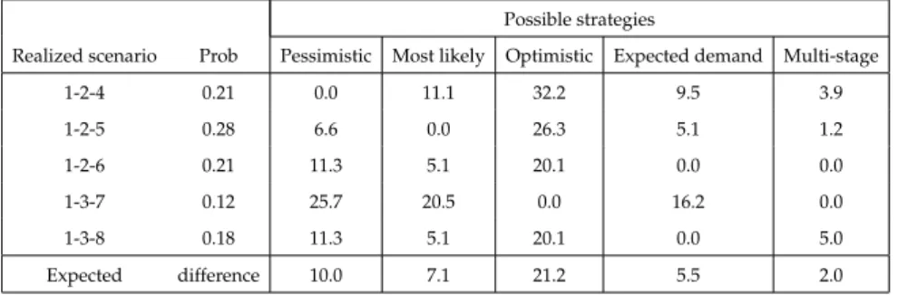
Another possible measure that can be used to evaluate the performance of options is the relative regret which gives the percentage difference of the total profit of the option to the profit of the optimal option in that scenario. However, we need to give a value to ξ in order to calculate this value for all possible options. Let us take a considerably small ξ = 10. Then, Table 2.2 gives the relative regret for each possible scenario. As Table 2.2 shows, the relative regret
Table 2.2: Relative regret of several strategies in different scenarios
Possible strategies
Realized scenario Prob Pessimistic Most likely Optimistic Expected demand Multi-stage
1-2-4 0.21 0.0 11.1 32.2 9.5 3.9 1-2-5 0.28 6.6 0.0 26.3 5.1 1.2 1-2-6 0.21 11.3 5.1 20.1 0.0 0.0 1-3-7 0.12 25.7 20.5 0.0 16.2 0.0 1-3-8 0.18 11.3 5.1 20.1 0.0 5.0 Expected difference 10.0 7.1 21.2 5.5 2.0
CHAPTER 2. PROBLEM DEFINITION AND LITERATURE REVIEW 12
option does not coincide with the scenario that it expects to happen. Moreover, in all cases multi-stage approach gives a profit value which is within 5% of the actual optimum profit while others may deviate up to 32%. Therefore, using a multi-stage approach instead of using fixed demand values may significantly improve the achieved results.
In addition to using multi-stage approach, using controllable processing times also increases the solution quality. For instance, for the given problem parameters, the multi-stage stochastic profit would decrease to 540 for every scenario if the processing times were fixed. This clearly indicates that the controllable processing times would enlarge the solution space such that we could utilize the limited capacity of the production resources more effectively.
2.4
Master Production Scheduling and
Avail-able to Promise
Master Production Schedules (MPS) assume infinite capacity and fixed processing times. The literature of MPS generally focuses on the length of frozen period, i.e. the number of periods in which the production scheduling decisions will not be altered even though there is a change in inputs, on stability issues of the MPS, and demand uncertainty. Sridharan et al. [33] consider the effect of the length of the frozen zone on production and inventory costs and also suggest that an order based freezing method is superior to a period based freezing method. Sridharan et al. [32] investigate the effects of several decision variables such as the freezing method, length of the frozen zone, and the length of the planning horizon. Tang and Grubbstr¨om [34] also study the effects of the length of the frozen period.
ATP problems consider decisions similar to our problem such as determining the amount of demand that will be satisfied, setting the due dates and planning resources which our problem also considers. A review of ATP problems can be found in Framinan and Leisten [15]. According to the classification of Framinan and Leisten [15], our problem has a similar structure with ATP problems using
CHAPTER 2. PROBLEM DEFINITION AND LITERATURE REVIEW 13
flexible due dates with a postponement penalty and flexible resources (we have flexible production capacity due to controllable processing times).
In this chapter, we defined the problem and explained the related literature, in the next chapter, we will give the formulations that we proposed and the sub-problems that we analyzed.
Chapter 3
The Stochastic Model
As we explained in the problem definition, we have a capacitated version of the MPS where the demand is uncertain and the processing times are controllable. Thus, the necessary decisions in the problem are how much to produce, when to produce, and the processing times during production. In this chapter, we give the main formulation that decides on when to produce and how much to produce assuming that the structure of the objective function is given. After that we introduce an equivalent linear version of the main formulation. Then, we introduce two subproblems: The first one is used to decide on the optimal processing times and to define the objective function of the main formulation whereas the second one reduces the size of the formulation. Finally, we give an alternative linearization of the main formulation using the results we have obtained.
3.1
The Multi-Stage Stochastic Programming
Formulation
We begin with defining the parameters of the problem. Let T be the number of periods in the planning horizon. Let N be the set of nodes of the scenario tree and
CHAPTER 3. THE STOCHASTIC MODEL 15
Nt be the set of the nodes of period t = 1, 2, ..., T . Suppose that the anticipated
demand at node i in N is denoted as diand the total demand (
P
i∈Ndi) is denoted
as d. For node i in N , let Di be the set of descendants of i including i, Bi be
the set of predecessors of i including i and finally, let γi denote the probability of
realization of node i (γ1 = 1). For i ∈ N and j ∈ Di, let Pij be the set of nodes
on the path from i to j in the scenario tree. Let si be the period of node i.
In addition to the parameters that are defined above, we will refresh some parameters that are already defined in Chapter 2 and will be used in the model. Let h be the unit profit excluding the compression and postponement costs, p be the processing time of a job with minimum compression cost, u be the maximum compression amount, and C be the capacity. We assume that h, p and C are positive and u is non-negative. Let kmax be the maximum number of jobs that
can be produced without violating the capacity constraint, i.e., kmax =
j
C p−u
k . Let Π(k) be the total profit when k jobs are produced at a node excluding the cost of postponement. Let b(t) be the cost of postponing one job for t periods. We assume that b(t) is a convex function with b(0) = 0. For the time being, we will assume that Π(k) is given for all possible values of k but later, we will explain how this value is calculated. The decision variables of the model are:
yj = Amount of production in j, j ∈ N ,
xij = Amount of dj that is processed in i, i ∈ N , j ∈ Bi,
zj = Amount of dj that will be satisfied, j ∈ N .
Then, the formulation for the stochastic problem (named as SF) is as follows:
M ax X i∈N γi· (Π(yi) − X j∈Bi b(si− sj)xij) s.t. X j∈Bi xij = yi ∀i ∈ N (3.1.1) (SF ) X i∈Pjm xij = zj ∀m ∈ NT ∩ Dj, j ∈ N (3.1.2) zj ≤ dj ∀j ∈ N (3.1.3) yj ≤ kmax ∀j ∈ N (3.1.4)
CHAPTER 3. THE STOCHASTIC MODEL 16
xij ∈ Z+ ∀ i ∈ N, j ∈ Bi
yi ∈ Z+ ∀i ∈ N
zi ∈ Z+ ∀i ∈ N.
The objective of SF is to maximize the total expected profit. Constraint (3.1.1) links xij and yi. It sums up the demand of j that is produced in node
i for all possible j values, i.e., all predecessors of node i including node i. This value is equal to the production amount in node i. Constraint (3.1.2) ensures that for each possible path that starts from node j and end at a descendant leaf node, the amount of j’s demand that is satisfied is the same as the amount of j’s demand that is produced along the path. Finally, Constraint (3.1.3) is the demand constraint and (3.1.4) is the capacity constraint.
As we will prove later, the objective function of SF is concave so it is a non-linear mixed integer formulation which necessitates a non-non-linear mixed integer solver. A directly linearized version of SF (SFL1) is as follows:
wik =
(
1 if k jobs are produced in node i
0 otherwise, i ∈ N, k ∈ {0, 1, ..., kmax}. Suppose that xij and zj are defined as before.
M ax X i∈N γi· ( kmax X k=0 Π(k) · wik− X j∈Bi b(si− sj)xij) s.t. kmax X k=0 wik = 1 ∀i ∈ N (3.1.5) (SF L1) X j∈Bi xij = kmax X k=0 k · wik ∀i ∈ N (3.1.6) X i∈Pjm xij = zj ∀m ∈ NT ∩ Dj, j ∈ N (3.1.7) zj ≤ dj ∀j ∈ N (3.1.8) xij ∈ Z+ ∀ i ∈ N, j ∈ Bi zi ∈ Z+ ∀i ∈ N wik ∈ {0, 1} ∀i ∈ N, k ∈ {0, 1, ..., kmax}.
CHAPTER 3. THE STOCHASTIC MODEL 17
The only difference between SF and SFL1 is formulating the integer variables as weighted sum of binaries. Constraint (3.1.5) guarantees that a node can have a single production amount. Since wikvalues are defined among feasible production
amounts, there is no need for constraint (3.1.4) of SF in SFL1.
At this point, we take the possible number of jobs that will be produced at a node as 0 to kmax which is the maximum number of jobs that can be produced
without violating the capacity of that node. Moreover, the compression amounts cannot be directly determined from the output of the model. In the following section, we will introduce two sub-problems which will be used to reduce the possible number of jobs and to calculate the optimal compression amounts.
3.2
Two Sub-problems
In this section, we introduce two sub-problems; the first sub-problem is the sin-gle period capacitated deterministic scheduling problem with cost minimization objective. The results that we obtain from this problem will be used to define the optimal compression costs and the Π(k) values.
3.2.1
The Single Period Capacitated Deterministic
Schedul-ing Problem with Cost Minimization Objective
This problem corresponds to a single machine (or work center), single product type problem where the machine has a finite capacity of C. Suppose that the processing time of a job which has the minimum compression cost is p and the maximum compressibility of the job is u. Let n be a positive integer such that n ≤ kmax. Suppose that there are n jobs in the work center. Let cj be the
compression amount of job j in {1, ..., n}. Recall that f is the compression cost function that is defined in Chapter 2. Then, the formulation of this subproblem
CHAPTER 3. THE STOCHASTIC MODEL 18 is: M in n X j=1 f (cj) s.t. cj ≤ u ∀j ∈ {1, ..., n} (3.2.1) n X j=1 (p − cj) ≤ C (3.2.2) cj ∈ R+ ∀ j ∈ {1, ..., n}.
The objective is to find the compression amounts for the jobs so that the total compression cost is minimized. (3.2.1) is the maximum compressibility constraint. (3.2.2) is the capacity constraint. Proposition 3.1 characterizes the optimal solu-tion of this problem.
Proposition 3.1. Let n be a positive integer with n · (p − u) ≤ C. If n jobs are to be processed in a work center, then the optimal compression amount of all the jobs is equal to max{p − Cn, 0}.
Proof. First, we show that the compression amount is equal for all the jobs in the work center. Let c be an optimal solution. Suppose to the contrary that there exist jobs i and j such that ci > cj. Let ¯c be the same as c except ¯ci =
¯ cj =
ci+cj
2 . The solution ¯c is feasible and by strict convexity of the cost function,
f ( ¯ci)+f ( ¯cj) < f (ci)+f (cj). This contradicts the optimality of the initial solution
c. Now it follows immediately that cj = max{p − Cn, 0} for all j = 1, ..., n is an
optimal solution.
The Proposition 3.1 is intuitive. In a strict convex function, the more a compression amount is, the more the marginal compression cost that will be incurred. Thus, in order to minimize the compression cost, the necessary com-pression amount (n · p − C) will be evenly distributed among all jobs. Using Proposition 3.1, it is possible to find the optimal compression amounts for jobs given the optimal allocation of jobs to the nodes. Thus, given the solution of SF, it is possible to find the compression amounts of jobs using this proposition.
As stated before, Π(k) function was considered as given when the main for-mulation is explained. Using Corollary 3.1, which makes use of Proposition 3.1,
CHAPTER 3. THE STOCHASTIC MODEL 19
we come up with the total cost and total profit functions of a node given the number of allocated jobs. As a remark, one should consider that each node can be modeled as a single work center once the allocation is available. For x ∈ R+,
let Π(x) = x · h − Φ(x) where Φ(x) = ( x · κ · (p − C x) a b if x > C p, 0 otherwise.
Corollary 3.1. Let n be a positive integer that satisfies n · (p − u) ≤ C. If n jobs are to be processed at a work center, then the total profit at the work center is Π(n) and the total compression cost when n jobs are processed in the work center is Φ(n).
Using Corollary 3.1, the profit function is calculated for all possible values of job numbers at a node and hence given as an input to the main formulation. The following sub-section will be used to define the threshold value.
3.2.2
The Single Period Capacitated Deterministic
Prob-lem with Profit Maximization Objective
In this problem, we have a single machine (or work center) with finite capacity C and a single period with infinite demand. The objective is to maximize the total profit. Let the threshold value, denoted by τ , be the optimal number of jobs that will be produced at the work center so that the total profit is maximized. Then, the formulation of the problem is:
max Π(n) s.t. n ≤ kmax
n ∈ Z+.
The value of τ depends on both the available capacity and relative profit gain of producing one more job. One should note that there is a trade-off between the revenue gained by increasing the number of jobs at a work center and the increase in the compression costs incurred in order to produce all these jobs. Thus, the
CHAPTER 3. THE STOCHASTIC MODEL 20
threshold value is the optimum production amount given the capacity of the work center.
We can simply use enumeration to come up with τ in O(kmax) time. However,
Lemma 3.1 gives the structure of the Π function when the compression amount of jobs are non-zero and Proposition 3.2, which gives the necessary and sufficient condition for the threshold value, can also be used to compute τ immediately. Lemma 3.1. Let Π : (0, +∞) → R be the profit function. The following proper-ties hold:
1) Π(x) is continuously differentiable at all points, 2) Π(x) is concave, 3) If h < κ · pab, there exists x in (C p, +∞) such that dΠ(x) dx = 0. Proof. Let Πc: (C p, +∞) → R be such that Π c(x) = x · h − x · κ · (p −C x) a b. Then, Π(x) = ( Πc(x) if x > Cp, x · h otherwise.
When x < Cp, Π(x) is linear and when x > Cp, Πc(x) is a smooth function since
x 6= 0. Therefore, the only point that needs consideration is x = Cp. The first derivative of the Πc function with respect to x is:
dΠc(x) dx = h − κ · (p − C x) a b − a b · κ · (p − C x) a b−1· C x.
The right derivative of Π(x) at x = Cp is h and the left derivative of Π(x) at x = Cp is also h. Therefore Π(x) is continuously differentiable at all points.
The second derivative of Πc(x) with respect to x is:
d2Πc(x) dx2 = − a b·κ·(p− C x) a b−1·C x2− a b·( a b−1)·κ·(p− C x) a b−2·C 2 x3+ a b·κ·(p− C x) a b−1·C x2 = −a b · ( a b − 1) · κ · (p − C x) a b−2· C 2 x3 ≤ 0
since a > b and x ≥ Cp, dΠdxc(x) is decreasing. Moreover, hx is non-increasing. In addition to those, the derivative function of Π(x) is continuous. Hence, dΠ(x)dx is monotonically non-increasing and continuous which means Π(x) is concave.
CHAPTER 3. THE STOCHASTIC MODEL 21
Now suppose that h < κ · pab. When x tends to C
p, dΠc(x)
dx > 0 and when x
tends to infinity, dΠdxc(x) < 0 since h < κ · pab. In addition to that, the derivative
function is continuous. Then, by the intermediate value theorem, there exists x∗ in (C
p, +∞) such that
dΠc(x∗)
dx = 0. Since Π(x) has the same values as Π
c(x) on
the domain (Cp, +∞), then dΠ(xdx∗) = 0.
Lemma 3.1 shows that the profit function is concave. It also shows that it always has a critical point within its domain if h < κ · pab. Thus, one can find this
critical point and by concavity this critical point is the maximizing point within a continuous domain if h < κ · pab. Obviously, this does not immediately tell what
the τ value is since τ is the maximum value defined among only integer points. Moreover, it does not consider the capacity constraint. However, Proposition 3.2 uses Lemma 3.1 to come up with the actual threshold value. Let kmin =
j
C p
k . Proposition 3.2. Suppose that h < κ · pab. Let x∗ be the critical point of Πc(x).
Then, τ = kmax if x∗ > kmax Πdx∗e if x∗ ≤ kmax and Π(dx∗e) > Π(bx∗c) Πbx∗c otherwise
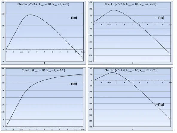
On the other hand, if h ≥ κ · pab, then τ = kmax.
Proof. While explaining the cases of the proof, we will refer to the charts in Figure 3.1. Consider first the case where h < κ · pab. The first condition immediately
follows from the concavity of the function. If x∗ > kmax, then the function is
increasing until kmax which is the largest feasible number of jobs that can be
produced. Thus in this case, τ = kmax.
The second case is where the critical point is within the domain of Proposition 3.1 and it is feasible (smaller than or equal to kmax). If x∗ < kmin + 1, this case
corresponds to charts c and d in Figure 3.1. As it can be also seen from the figures, the function is decreasing after kmin+ 1 and increasing before kmin. Thus, either
τ = kmin + 1 = dx∗e as illustrated in chart c or τ = kmin = bx∗c as illustrated
in chart d. Therefore, we need to check each one and take the one with higher profit as the threshold value. Similarly, if kmax≥ x∗ ≥ kmin+ 1, the critical point
CHAPTER 3. THE STOCHASTIC MODEL 22
is optimal for continuous case and rounding it down or up will give the integer optimum due to concavity of the function in this domain. Thus, the one with higher profit gives the threshold value. Chart a illustrates this case since x∗ is 3.2 which is greater than kmin + 1 = 3. So rounding it down gave a better solution
which means that the τ value is 3.
If h ≥ κ · pab, then the derivative of the Π function is always non-negatively
signed as illustrated in chart b of Figure 3.1. Thus, Π is monotonically non-decreasing. τ is the maximum feasible job number which is kmax.
-50 0 50 100 150 200 0 1 kmin τ=3 4 5 6 7 8 9 kmax x
Chart a (x*=3.2, kmax= 10, kmin=2, τ=3 )
Π(x) 0 50 100 150 200 250 300 350 400 0 1 kmin 3 4 5 6 7 8 9 kmax
Chart b (kmax= 10, kmin=2, τ=10 )
Π(x) -300 -250 -200 -150 -100 -50 0 50 100 150 0 1 kmin 3 4 5 6 7 8 9 kmax x
Chart c (x*=2.6, kmax= 10, kmin=2, τ=3 )
Π(x) -400 -350 -300 -250 -200 -150 -100 -50 0 50 100 0 1 kmin 3 4 5 6 7 8 9 kmax x
Chart d (x*=2.4, kmax= 10, kmin=2, τ=2 )
Π(x)
Figure 3.1: Profit charts in different cases
Example 2. Consider the problem given in Figure 2.1. Recall that f (y) = y32,
h = 60, p = 10, u = 4 and C = 36 in the problem. Then, this corresponds to the case where h > κpab. The threshold value is kmax = 6.
CHAPTER 3. THE STOCHASTIC MODEL 23
3.3
The Formulation with a Reduced Size
Using the threshold value, it is possible to reduce the size of the main formulation. Proposition 3.3 gives a necessary condition for the optimality of the main problem which will be used to reduce the formulation size.
Proposition 3.3. At an optimal solution to SF, the production amounts of all nodes are less than or equal to the threshold value, τ .
Proof. If τ = kmax, then it is infeasible to produce more than τ . If not, suppose
that there exists an optimal solution in which the production amount at a node is greater than τ . Then, we can simply improve the solution by decreasing the production amount to τ and reach a contradiction.
According to Proposition 3.3, the number of jobs that will be produced will be less than the threshold value at all nodes in the optimal solution. Thus, the maximum number of jobs that will be produced at a node decreases from kmax
to τ . Therefore, kmax in the main formulation is replaced by τ .
After explaining the main formulation and two sub-problems which are used to reduce problem size of the main formulation, to calculate Π(n) values as well as optimum compression amounts, we will introduce an alternative linearization to SF.
3.4
An Alternative Linearization of the
Stochas-tic Formulation (SF)
In this section, we give an alternative linearized version of SF. In this formula-tion, we write the integer variable yj as the sum of binary variables vik. Then,
CHAPTER 3. THE STOCHASTIC MODEL 24
vik =
(
1 if at least k jobs are produced in i
0 otherwise, i ∈ N, k ∈ {1, ..., τ },
xij = Amount of dj processed in i, i ∈ N , j ∈ Bi,
zj = Amount of dj that will be satisfied, j ∈ N .
Consequently, the alternative linear formulation (named as SFL2) is as follows:
M ax X i∈N γi· ( τ X k=1 (Π(k) − Π(k − 1)) · vik− X j∈Bi b(si− sj) · xij) s.t. vik ≥ vi(k+1) ∀i ∈ N, k ∈ {1, ..., τ − 1} (3.4.1) (SF L2) X j∈Bi xij = τ X k=1 vik ∀i ∈ N (3.4.2) X i∈Pjm xij = zj ∀m ∈ NT ∩ Dj, j ∈ N (3.4.3) zj ≤ dj ∀j ∈ N (3.4.4) xij ∈ Z+ ∀ i ∈ N, j ∈ Bi zi ∈ Z+ ∀i ∈ N vik ∈ {0, 1} ∀i ∈ N, k ∈ {1, ..., τ }.
Constraint (3.4.1) of SFL2 handles the fact that if at least k +1 jobs are processed at a node, then clearly at least k jobs will be processed. Constraint (3.4.2) has the same task as Constraint (3.1.1) but in it, the integer variable yi is written as
the sum of binary variables vik. The other constraints are the same as Constraint
(3.1.7) and (3.1.8) in SFL1.
SFL2 linearizes SF albeit at a cost of increased number of variables due to addition of vik’s and increased number of constraints due to addition of Constraint
(3.4.1). However, it is easy to get rid of Constraint (3.4.1) due to concavity of Π(x) and convexity of b(k). Let SFL3 be the same formulation as SFL2 without Constraint (3.4.1). Proposition 3.4 formalizes this idea.
Proposition 3.4. Let SFL2 and SFL3 be defined as above. Then, there exists an optimal solution for SFL3 which is also optimal for SFL2.
Proof. Let x∗ij, v∗ik, and zj∗ be an optimal solution for SFL3. Since SFL3 is a relaxation of SFL2, if there is an optimal solution for SFL3 which is feasible
CHAPTER 3. THE STOCHASTIC MODEL 25
for SFL2, then it is also optimal for SFL2. Now clearly x∗ij, vik∗, and z∗j satisfy constraints 3.4.2, 3.4.3,3.4.4 since SFL3 also includes these constraints. Then, if vik∗ satisfies 3.4.1, we are done. If not, suppose that Pτ
k=1v ∗ ik = n ∗ and let k in be defined as: ki1= min{k ∈ {1, ..., τ } : vik = 1} ki2= min{k ∈ {1, ..., τ } : vik = 1; k > ki1} .. . kin∗ = min{k ∈ {1, ..., τ } : vik = 1; k > ki(n∗−1)}
Now consider the solution ¯xij = x∗ij, ¯zj = zj∗ and
¯ vin = ( vikin if n ≤ n ∗ 0 if n > n∗ i ∈ N, k ∈ {1, ..., τ } Now by definition, Pτ k=1v¯ik = n
∗ thus this solution satisfies 3.4.2. Moreover,
this solution satisfies 3.4.1 since ¯vik = 0 implies ¯vi(k+1) = 0 (otherwise leads to a
contradiction). Moreover, ¯vi(k+1) = 1 means ¯vik = 1 by definition of kin. Thus,
this new solution is feasible for SFL2 and clearly for SFL3. Now to show that it is optimal for SFL3, we need to consider the objective function value of it. The difference between the objective function of the old and new formulation is P i∈Nγi· ( Pτ k=1(Π(k) − Π(k − 1)) · (v ∗ ik− ¯vik) = γi· (Pn ∗ n=1((Π(kin) − Π(kin− 1)) − (Π(n) − Π(n − 1))).
As Lemma 3.1 suggests, Π(k) is a concave function, hence the first derivative is always non-increasing. Therefore, ((Π(kin) − Π(kin− 1)) ≤ (Π(n) − Π(n − 1)))
since by definition kin ≥ n. Thus, this solution is also optimal for SFL3 and
feasible for SFL2, hence it is optimal for SFL2.
SFL2 is always feasible since setting all variables to zero gives a feasible so-lution for it. Therefore, according to Proposition 3.4, there exists an optimal solution of SFL3 which is also optimal for SFL2. Thus, one can solve SFL3, find an optimal solution and convert the solution so that it is feasible for SFL2 via procedure (kin) that is proposed in the proof. Hence, the the solution obtained
is optimal for SFL2.
In this chapter, we first proposed a stochastic formulation and a linearized version of it. Afterwards, we analyzed two sub-problems to come up with the optimal processing times and profit function Π(k) and the threshold value. We
CHAPTER 3. THE STOCHASTIC MODEL 26
also obtained the result that Π(k) is concave which is used while forming SFL3. We also came up with τ value and reduced the size of the formulations that we propose. In the next chapter, we will introduce sufficient conditions for optimality and two special cases of the main problem which are polynomially solvable. Then we will discuss the complexity of our problem.
Chapter 4
On Easy Cases and Complexity
In this chapter, we first give some instances of the problem which are easily solvable. Then we introduce the case where there is no postponement cost and the case where the demands are deterministic. We prove the polynomiality of both cases. Finally, we have a negative result: The techniques that we used to determine the complexity of the easy cases is not applicable to the main problem.
4.1
Sufficient Conditions for Optimality
In this section, we will introduce some easy cases where the optimal solution can be found easily. Suppose that the demand at each node is less than the threshold value and equal to each other. Then by Proposition 4.1, the solution where each job is produced at its own node (the node in which the demand of the job is realized) is optimal.
Proposition 4.1. Suppose that, di < τ for all i in set N . If di = dj for all i and
j, then the solution where all the demand is satisfied and each job is produced at its own node is optimal.
Proof. Suppose that di = dj = n for all i and j in N but the solution is not
optimal. Then, there exists a better solution. Firstly, it is not possible to improve 27
CHAPTER 4. ON EASY CASES AND COMPLEXITY 28
the solution by decreasing the production amount because di < τ for all i in N .
Then there exists i and set M ⊂ Di such that adding a job to i from the nodes in
set M or adding a job from i to the nodes in set M improves the solution. Note that by definition, γi =Pk∈Mγk.
Case 1: An improvement is achieved by adding a job to i from the nodes in set M . Then, the change in cost for i is Φ(n+1)−Φ(n) and the cost change for all nodes in M is Φ(n)−Φ(n−1). Thus the total change in cost is ∆f = γi·(Φ(n+1)−Φ(n))−
P
k∈Mγk·(Φ(n)−Φ(n−1)) = γi·(Φ(n+1)−Φ(n))−(Φ(n)−Φ(n−1))·
P
k∈Mγk =
γi·((Φ(n+1)−Φ(n))−(Φ(n)−Φ(n−1))) = γi·((Φ(n+1)+Φ(n−1)−2Φ(n))) > 0
by strict convexity of the cost function. However, this contradicts with the fact that this case improves the solution.
Case 2: An improvement is achieved by adding a job from i to the nodes in set M . A similar contradiction is reached for this case just as case 1.
Therefore, there does not exist such i and set M . Hence, the solution is optimal.
Another easy to solve case is where the demand exceeds the threshold value at all of the nodes. A sufficient condition for optimality in this case is given in Proposition 4.2.
Proposition 4.2. Suppose that, the demand exceeds the threshold value for all nodes in the scenario tree. Then, the solution where τ jobs are produced at all nodes is optimal.
Proof. In the solution proposed, τ jobs will be produced in all nodes. For any node, the optimal number to produce is τ by definition. Thus, adding a job to or subtracting a job from a node will worsen the objective function value. Thus, the solution is optimal.
Using Propositions 4.1 and 4.2, one can immediately find the optimal solution when the corresponding easy cases are encountered.
CHAPTER 4. ON EASY CASES AND COMPLEXITY 29
4.2
Stochastic Problem with no Postponement
Cost
We propose a special formulation for the stochastic problem without any post-ponement cost. This special formulation comes out with a simple observation: the number of jobs that will be produced along a path starting from the root node will be less than or equal to the total demand along the path. Having this observation in mind, one can define the necessary decision variable as the amount of production at a node without considering where the demands of this produc-tion are realized once the postponement is no longer costly. Let yi denote the
production at node i in N . Then the alternative formulation is as follows:
M ax X i∈N γi· Π(yi) s.t. X j∈P1i yj ≤ X j∈P1i dj ∀i ∈ N (4.2.1) (SF 2) yi ≤ τ ∀i ∈ N (4.2.2) yi ∈ Z+ ∀i ∈ N
The objective is to maximize the total expected profit and Constraint (4.2.1) guarantees that the production amount along a path does not exceed the total demand. Constraint (4.2.2) is the capacity constraint.
SF2 cannot be solved in a commercial solver for reasonable input sizes since it is a non-linear mixed integer problem. However, this formulation will be used to show the complexity of the stochastic problem without postponement cost since it has a special structure. Lemma 4.1 shows the special structure of its constraint matrix.
Lemma 4.1. Constraint matrix of SF2 is totally unimodular.
Proof. The constraint matrix consists of two parts, one (sub-matrix 1) is identity matrix and the other(sub-matrix 2) is due to Constraint (4.2.1). If we sort the
CHAPTER 4. ON EASY CASES AND COMPLEXITY 30
rows of sub-matrix 2 in a depth-first search basis, then this sub-matrix satisfies consecutive 1’s property and thus is totally unimodular [16]. Moreover, sub-matrix 1 is an identity sub-matrix. Thus, the constraint sub-matrix is totally unimodular.
Theorem 4.1. Stochastic problem with no postponement cost is polynomially solvable.
Proof. In the objective function, for i in N , γi · Π(yi) is concave so multiplying
it by -1, we obtain a convex function. Their summation generates a convex separable objective function (with minimization objective or concave separable objective function with maximization). Moreover, by Lemma 4.1, the constraint matrix is totally unimodular. Thus according to Hochbaum and Shantikumar [20], stochastic problem is polynomially solvable.
4.3
The Deterministic Problem
In this section, we consider the problem with deterministic demand realizations. If we adjust SF for the deterministic case, we obtain the following decision variables:
yj = Amount of production in period j
xij = Amount of demand of j that is processed in i, i ∈ {1, ..., T }, j ∈ {1, ..., i}.
Then, the formulation for the deterministic case (named as DF) is as follows:
M ax T X i=1 (Π(yi) − i X j=1 b(si− sj)xij) s.t. i X j=1 xij = yi ∀i ∈ {1, ..., T } (4.3.1) (DF ) T X i=j xij ≤ dj ∀j ∈ {1, ..., T } (4.3.2)
CHAPTER 4. ON EASY CASES AND COMPLEXITY 31
yj ≤ τ ∀j ∈ {1, ..., T } (4.3.3)
xij ∈ Z+ ∀i ∈ {1, ..., T }, j ∈ {1, ..., i}
yi ∈ Z+ ∀i ∈ {1, ..., T }
Constraints have the same tasks as SF but the only difference is that instead of different scenarios, there is a single scenario, i.e., the scenario tree is a path. Lemma 4.2. Constraint matrix of DF is totally unimodular.
Proof. Firstly, the constraint matrix clearly consists of 1’s -1’s and 0’s. Given a set of rows of the constraint matrix, put the rows of Constraint Set (4.3.1) into partition 1 and the rows of Constraint Sets (4.3.2) and (4.3.3) into partition 2. Then the difference of the sums of rows of partition 1 and 2 has entries that are equal to either 1, 0 or -1. Therefore, the matrix is totally unimodular [35]. Theorem 4.2. The deterministic problem is polynomially solvable.
Proof. In the objective function, for i in {1, ..., T }, Π(yi) is concave and b(x) is
convex which leads to -b(x) being concave. Therefore, the objective function is concave separable and so multiplying it by -1, we obtain minimization of sum of convex separable functions. Moreover, by Lemma 4.2, the constraint matrix is totally unimodular. Thus, according to Hochbaum and Shantikumar [20], deter-ministic version of the problem is also polynomially solvable.
4.4
The Structure of Stochastic Formulation SF
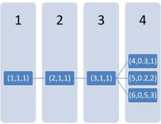
In the previous sections, we proved that some special cases of the problem are polynomially solvable. We achieved this by suggesting formulations with totally unimodular constraint matrices and concave separable objective functions. In this section, we first show that this approach cannot be applied to the general problem because the constraint matrix of SF may not be totally unimodular. Example 3. Consider the very simple scenario tree given in Figure 4.1. The co-efficient matrix of the corresponding stochastic formulation of this scenario tree
CHAPTER 4. ON EASY CASES AND COMPLEXITY 32
4
3
2
1
(1,1,1) (2,1,1) (3,1,1) (4,0.3,1) (5,0.2,2) (6,0,5,3)Figure 4.1: A counter example for totally unimodularity of constraint matrix of SF
is given in Table 4.1:
Table 4.1: Constraint coefficient matrix for stochastic formulation of Figure 4.1
Ctr x11 x21 x22 x31 x32 x33 x41 x42 x43 x44 x51 x52 x53 x55 x61 x62 x63 x66 y1 y2 y3 y4 y5 y6 z1 z2 z3 z4 z5 z6 1 1 0 0 0 0 0 0 0 0 0 0 0 0 0 0 0 0 0 -1 0 0 0 0 0 0 0 0 0 0 0 2 0 1 1 0 0 0 0 0 0 0 0 0 0 0 0 0 0 0 0 -1 0 0 0 0 0 0 0 0 0 0 3 0 0 0 1 1 1 0 0 0 0 0 0 0 0 0 0 0 0 0 0 -1 0 0 0 0 0 0 0 0 0 4 0 0 0 0 0 0 1 1 1 1 0 0 0 0 0 0 0 0 0 0 0 -1 0 0 0 0 0 0 0 0 5 0 0 0 0 0 0 0 0 0 0 1 1 1 1 0 0 0 0 0 0 0 0 -1 0 0 0 0 0 0 0 6 0 0 0 0 0 0 0 0 0 0 0 0 0 0 1 1 1 1 0 0 0 0 0 - 1 0 0 0 0 0 0 7 1 1 0 1 0 0 1 0 0 0 0 0 0 0 0 0 0 0 0 0 0 0 0 0 -1 0 0 0 0 0 8 1 1 0 1 0 0 0 0 0 0 1 0 0 0 0 0 0 0 0 0 0 0 0 0 -1 0 0 0 0 0 9 1 1 0 1 0 0 0 0 0 0 0 0 0 0 1 0 0 0 0 0 0 0 0 0 -1 0 0 0 0 0 10 0 0 1 0 1 0 0 1 0 0 0 0 0 0 0 0 0 0 0 0 0 0 0 0 0 -1 0 0 0 0 11 0 0 1 0 1 0 0 0 0 0 0 1 0 0 0 0 0 0 0 0 0 0 0 0 0 -1 0 0 0 0 12 0 0 1 0 1 0 0 0 0 0 0 0 0 0 0 1 0 0 0 0 0 0 0 0 0 -1 0 0 0 0 13 0 0 0 0 0 1 0 0 1 0 0 0 0 0 0 0 0 0 0 0 0 0 0 0 0 0 -1 0 0 0 14 0 0 0 0 0 1 0 0 0 0 0 0 1 0 0 0 0 0 0 0 0 0 0 0 0 0 -1 0 0 0 15 0 0 0 0 0 1 0 0 0 0 0 0 0 0 0 0 1 0 0 0 0 0 0 0 0 0 -1 0 0 0 16 0 0 0 0 0 0 0 0 0 1 0 0 0 0 0 0 0 0 0 0 0 0 0 0 0 0 0 -1 0 0 17 0 0 0 0 0 0 0 0 0 0 0 0 0 1 0 0 0 0 0 0 0 0 0 0 0 0 0 0 -1 0 18 0 0 0 0 0 0 0 0 0 0 0 0 0 0 0 0 0 1 0 0 0 0 0 0 0 0 0 0 0 -1
For this constraint matrix to be totally unimodular, we need to have all sub-matrices to have determinant -1,0 or 1. However, the following sub-matrix of this coefficient matrix has determinant 2:
CHAPTER 4. ON EASY CASES AND COMPLEXITY 33 0 0 0 1 1 0 0 0 0 0 0 0 0 0 1 1 0 0 0 0 0 0 0 0 0 1 1 1 0 0 1 0 0 0 0 0 1 0 0 0 0 0 0 1 0 0 1 0 0 0 1 0 0 0 0 1 0 0 0 0 0 0 1 0 0 1 0 1 0 0 0 0 0 0 1 0 0 0 1 0 0
Therefore, the constraint matrix of SF may not be totally unimodular. This directly implies that the constraint matrix of SFL3 may not be TU, either because the same sub-matrix exists in the coefficient matrix of SFL3 for the problem given in Figure 4.1.
As this approach failed for SF and SFL3, we sought another structure that is suggested in Hemmecke et al. [19]. In that paper, authors show the polynomiality of n-fold integer minimization problem. Let A and B be two matrices with the same number of columns. Then n-fold matrix of the ordered pair A and B is given as: B B B . . . B A 0 0 . . . 0 0 A 0 . . . 0 0 0 A . . . 0 .. . ... ... . .. ... 0 0 0 0 A
If the constraint matrix has such a structure, it can be decomposed into n smaller problems once the coupling constraints are dropped, hence this is called n-fold integer program. Hemmecke et al. [19] showed that convex integer programs having this property are polynomially solvable. Thus, we checked whether the
CHAPTER 4. ON EASY CASES AND COMPLEXITY 34
constraint matrix of SF has such a structure. However, the following example shows that SF may not have this property:
2
1
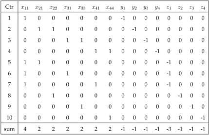
(1,1,1) (2,0.3,1) (3,0.2,2) (4,0.5,3)Figure 4.2: A counter example for structure in Hemmecke et al. [19] Example 4. Consider the scenario tree given in Figure 4.2. The constraint matrix corresponding to this scenario tree is given in Table 4.2.
Table 4.2: Constraint coefficient matrix for stochastic formulation of Figure 4.2
Ctr x11 x21 x22 x31 x33 x41 x44 y1 y2 y3 y4 z1 z2 z3 z4 1 1 0 0 0 0 0 0 -1 0 0 0 0 0 0 0 2 0 1 1 0 0 0 0 0 -1 0 0 0 0 0 0 3 0 0 0 1 1 0 0 0 0 -1 0 0 0 0 0 4 0 0 0 0 0 1 1 0 0 0 -1 0 0 0 0 5 1 1 0 0 0 0 0 0 0 0 0 -1 0 0 0 6 1 0 0 1 0 0 0 0 0 0 0 -1 0 0 0 7 1 0 0 0 0 1 0 0 0 0 0 -1 0 0 0 8 0 0 1 0 0 0 0 0 0 0 0 0 -1 0 0 9 0 0 0 0 1 0 0 0 0 0 0 0 0 -1 0 10 0 0 0 0 0 0 1 0 0 0 0 0 0 0 -1 sum 4 2 2 2 2 2 2 -1 -1 -1 -1 -3 -1 -1 -1
In order to have the structure that is sought, we need identical sub-matrices inside the constraint matrix. Therefore, we need at least n column pairs with the same column sum in order to have n such identical matrices. However, as Table 4.2 displays, the sum of first column is 4 and there is no other column with such column sum. Thus, SF may not possess the structure given in Hemmecke et al. [19] except for trivial n=1. Hence, we cannot claim that the problem is polynomially solvable. As a result, the complexity of the general stochastic problem with postponement cost is still open.
CHAPTER 4. ON EASY CASES AND COMPLEXITY 35
In this chapter, we introduced some sufficient conditions and proved the poly-nomiality of two special cases of the problem. In the next chapter, we will give the results of our computational study.