Minimazing the total completion time in a two stage flow shop with a single setup server

(1)

i

MINIMIZING THE TOTAL COMPLETION TIME IN A TWO

STAGE FLOW SHOP WITH A SINGLE SETUP SERVER

A THESİS

SUBMITTED TO THE DEPARTMENT OF INDUSTRIAL ENGINEERING

AND THE GRADUATE SCHOOL OF ENGINEERING AND SCIENCE

OF BILKENT UNIVERSITY

IN PARTIAL FULFILLMENT OF THE REQUIREMENTS

FOR THE DEGREE OF

MASTER OF SCIENCE

By

Muhammet KOLAY

July, 2012

(2)

ii

ABSTRACT

MINIMIZING THE TOTAL COMPLETION TIME IN A TWO STAGE FLOW

SHOP WITH A SINGLE SETUP SERVER

Muhammet KOLAY M.S. in Industrial Engineering Supervisor: Prof.Dr.Ülkü Gürler

Supervisor: Assoc. Prof.Dr.Mehmet Rüştü Taner July, 2012

In this thesis, we study a two stage flow shop problem with a single server. All jobs are available for processing at time zero. Processing of a job is preceded by a sequence independent setup operation on both machines. The setup and processing times of all jobs on the two machines are given. All setups are performed by the same server who can perform one setup at a time. Setups cannot be performed simultaneously with job processing on the same machine. Once the setup is completed for a job, processing can automatically progress without any further need for the server. Setup for a job may start on the second machine before that job finishes its processing on the first machine. Preemption of setup or processing operations is not allowed. A job is completed when it finishes processing on the second machine. The objective is to schedule the setup and processing operations on the two machines in such a way that the total completion time is minimized. This problem is known to be strongly NP-hard [3]. We propose a new mixed integer programming formulation for small-sized instances and a Variable Neighborhood Search (VNS) mechanism for larger problems. We also develop several lower bounds to help assess the quality of heuristic solutions on large instances for which optimum solutions are not available. Experimental results indicate that the proposed heuristic provides reasonably effective solutions in a variety of instances and it is very efficient in terms of computational requirements.

Keywords: machine scheduling, flow shop, single setup server, total completion time, variable neighborhood search.

(3)

iii

ÖZET

TEK SUNUCULU İKİ AŞAMALI SERİ AKIŞDA

TOPLAM TAMAMLANMA ZAMANINI EN AZLAMAK

Muhammet Kolay

Endüstri Mühendisliği, Yüksek Lisans Tez Yöneticisi: Prof. Dr. Ülkü Gürler Tez Yöneticisi: Doç. Dr. Mehmet Rüştü Taner

Temmuz 2012

Bu tez kapsamında; tek sunuculu iki aşamalı seri akış problemi çalışılmıştır. Tüm işler sıfır zamanında işlem görmek üzere hazırdırlar. Her iki makine üzerinde, bir iş için işleme başlamadan önce sıradan bağımsız olarak hazırlık işlemleri yapılmaktadır. Bütün işler için, işlem süreleri ve hazırlık süreleri verilmiştir. Tüm hazırlık işlemleri, tek seferde sadece bir iş için hazırlık yapabilen bir sunucu tarafından yapılmaktadır. Aynı makine üzerinde bir işe ait işlem operasyonu devam ederken aynı anda hazırlık işlemi yapılamamaktadır. Bir işin hazırlığı tamamlandığı zaman, işlem operasyonu sunucuya ihtiyaç duyulmadan otomatik olarak yapılabilmektedir. Bir işin ikinci makinede hazırlanmasına, aynı işin birinci makinedeki işlemi devam ederken başlanabilmektedir. Hazırlık sürelerinin ve işlem sürelerinin bölünerek yapılmasına müsaade edilmemektedir. Bir iş, ikinci makinedeki işlemi bittiğinde tamamlanmış olarak kabul edilir. Problemin amacı verilen tüm işleri iki makine üzerinde toplam tamamlanma zamanlarını en azlayacak şekilde çizelgelemektir. Bu problem NP-zor bir problemdir. Küçük boyutlu problemleri çözmek için karışık tam sayılı programlama modeli, büyük problemleri çözebilmek için ise sezgisel Değişken Komşu Arama mekanizması önerilmiştir. Ayrıca, sezgisel algoritmaların performansını en iyi sonuçların elde edilemediği büyük problemlerde değerlendirebilmek amacıyla, alt sınırlar geliştirilmiştir. Yapılan deneylerin sonucunda; önerilen sezgisel algoritmaların farklı örnek çeşitlerinde etkili sonuçlar verdiği ve hesaplanabilirlik açısından çok etkili oldukları görülmüştür.

Anahtar sözcükler: makine çizelgeleme, seri akış, tek hazırlık sunucusu, toplam tamamlanma zamanı, değişken komşu arama.

(4)

iv

Acknowledgement

Foremost, I would like to express my deepest and most sincere gratitude to my advisor Assoc. Prof. Dr. Mehmet Rüştü Taner for his invaluable guidance, encouragement and motivation during my graduate study. I could not have imagined having better mentor for my M.S study.

I would like to express my sincere thanks to Professor Ulku Gurler for accepting to serve as one of my supervisors in the last few months of my study and for her insightful comments that helped to improve the readability of this thesis.

I am also grateful to Assoc. Prof. Dr. Oya Ekin Karaşan and Asst. Prof. Dr. Sinan Gürel for accepting to read and review this thesis and for their invaluable suggestions.

I am indebted to Selva Şelfun for her incredible support, patience and understanding throughout my M.S study.

Many thanks to Betül Kolay, Ahmet Kolay, Kamil Kolay and Murat Kolay for their moral support and help during my graduate study. I am lucky to have them as a part of my family.

Last but not the least; I would like to thank to my lovely family. The constant inspiration and guidance kept me focused and motivated. I am grateful to my dad Mustafa Kolay for giving me the life I ever dreamed. I can't express my gratitude for my mom Niğmet Kolay in words, whose unconditional love has been my greatest strength. The constant love and supports of my brother Alper Kolay and my sister İrem Tuana Kolay are sincerely acknowledged.

(5)

v

List of Figures

3.1 Optimal Solution for the Given Example ... 9

3.2 Example of an Optimal Schedule for the Special Case ... 14

4.1 Possible Idle Times for the LB 3 ... 19

4.2 Solution Representation for the Given Example ... 22

4.3 Flow Chart of VNS 1 Algorithm ... 37

4.4 Flow Chart of Insert/Pairwise Interchange Methods for VNS 1 and VNS 2 ... 39

4.5 Flow Chart of First Machine Move/Second Machine Move Methods for VNS 1 and VNS 2 ... 40

5.1 Percentage Deviation of Lower Bounds from Optimal Solutions for N=5 ... 45

5.4 Average Running Time of LB 4 according to N ... 46

5.5 Percentage Deviation of LB from Optimal Solutions according to R and N ... 47

5.6 Running Times of the Optimal Solutions according to R and N ... 48

5.7 Maximum and Average Percentage Deviation of Heuristics from Optimal .... 50

5.8 Maximum and Average Percentage Deviation of Best Lower Bound from Heuristic according to N ... 53

5.9 Maximum and Average Percentage Deviation of Best Lower Bound from Heuristic according to R ... 53

(7)

vii

5.10 Comparison of Running Times of LB and Heuristic for R=0.01, 0.05 and 0.1 ... 54

5.11 Comparison of VNS 1 and VNS 2 according to N ... 57

(8)

viii

List of Tables

3.1 Data for Given Example ... 9

4.1 Data for Toy Problem ... 16

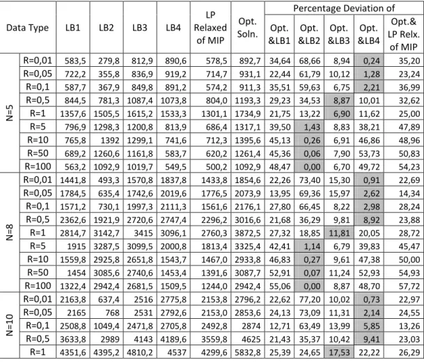
5.1 Results for Comparison of Lower Bounds with Optimal Solutions ... 44

5.2 Results for Comparison of Best Lower Bound with Optimal Solutions ... 47

5.3 Results for Comparison of Heuristic Algorithms with Optimal Solutions ... 49

5.4 Results for Comparison of Heuristic Algorithm with Best LB – 1/2... 51

5.5 Results for Comparison of Heuristic Algorithm with Best LB – 2/2... 52

5.6 Comparison of VNS 1 and VNS 2 according to Best Lower Bound – 1/2 ... 56

5.7 Comparison of VNS 1 and VNS 2 according to Best Lower Bound – 2/2 ... 57

A.1 Computational Results for N=5-1/3 ... 66

(9)

ix

(10)

1

Chapter 1 Introduction

In many manufacturing facilities and assembly lines, each job has to go through a series of operations. Mostly, these operations have to be done in the same order for all jobs which implies that, each job gets to be processed on every machine in the same order. Flow shop problems aim to schedule a given set of jobs on a number of machines in such a system so as to optimize a given criterion. Most researchers assume that, setup times can be included in the processing times or ignored entirely. Even though this assumption may be valid for some cases, there are still many applications where an explicit consideration of setup times is necessary. Some example cases in which setup times may significantly affect the operational planning activities are those involving tool change, die change, clean up, loading and unloading operations. .

Additionally in real life, most systems work semi-automatically, and this requires involvement of a server before or after processing operations. This may be the case in certain flow shop applications also. In these applications, setup operation for a job may be carried out before that job finishes its previous processing and arrives at the current machine. To avoid high labor expenses, a single server may be in charge of performing setups on multiple machines.

The main goal of our problem is to minimize the total completion time of all jobs. A flow shop environment is a good design for producing similar items in large quantities to stock. But usually, there tends to be little space along the production

(11)

2

line for work=in=process storage. This suggests that minimizing the total completion time is a particularly relevant objective in such a setting.

Differently from classical two stage flow shop, in our problem immediately before processing an operation, machine has to be prepared by the server for the operation, which is called setup. During setup, both the machine and the server will be occupied. All setups should be done by the single server who can perform at most one setup at a time. Server is responsible only for the setup operation, once the setup is completed, process is executed automatically without the server. A job is completed when the processing on the second machine is finished. The goal of the problem is to schedule the given set of jobs in order to minimize the total completion time.

Although there appeared some studies in the literature on parallel machine scheduling problems with a single server, the flow shop versions of these problems received much less attention from the research community. Lim et al. [1] consider single server in a two machine flow shop for the makespan objective. Although the classical two machine flow shop problem with the makespan objective is polynomially solvable [2], the version of the problem with a single setup server is known to be unary NP-Hard [3]. Lim et al. propose a number of heuristics to gain near optimal solutions for the problem with the makespan objective.

This thesis focuses on the total completion time objective in a two machine flow shop with a single setup server. Chapter 2 reviews the literature on scheduling problems with a single server. After presenting a formal definition of the problem at hand, a mixed integer programming model is proposed in Chapter 3 to solve small instances to optimality. Then, Chapter 4 presents the proposed heuristic algorithms to solve larger instances that cannot be solved via exact methods due to the curse of dimensionality. We also develop several lower bounds in this same chapter to help assess the quality of heuristic solutions on instances for which optimum solutions cannot be obtained. Chapter 5 presents the results of our computational study through which the proposed algorithms and lower bounds are tested. Finally, Chapter 6 concludes the thesis with a summary of the major findings and directions for possible future studies.

(12)

3

Chapter 2 Literature Review

In many manufacturing and assembly facilities each job has to undergo a series of operations. Often, these operations have to be done on all jobs in the same order implying that the jobs have to follow the same route. The machines are then assumed to be set up in series and the environment is referred to as a flow shop [4].

After publication of Johnson’s [2] classical paper, in which he proved that the two stage flow-shop problem with the makespan objective can be solved in polynomial time, many researchers focused on flow-shop problems. However, makespan is still the only objective function for which the two stage flow shop problem can be solved in polynomial time. For the classical flow-shop problem, Garey [5] shows that the problem is NP-hard with the total completion time as the objective criterion.

There are some studies in the literature that have an explicit consideration of setups. Setup times are classified as separable and non-separable. When setup times are separable from the processing times, they could be anticipatory (or detached). In the case of anticipatory (detached) setups, the setup of the next job can start as soon as a machine becomes free to process the job since the shop floor control system can identify the next job in the sequence. In such a situation, the idle time of a machine can be used to complete the setup of a job on a specific machine. In other situations, setup times are non-anticipatory (or attached) and the setup

(13)

4

operations can start only when the job arrives at a machine as the setup is attached to the job [6]. Setup times are also classified as sequence dependent and sequence independent. Setups are called sequence dependent, when the setup times change as a function of the job order. There is extensive literature on scheduling with setup times excellent reviews of which can be found in [6], [7] and [8].

In our problem, setup times are anticipatory and sequence independent. Additionally, a single setup server is responsible to carry out the setup operation. There are a number of studies on scheduling problems with a single server. Most of them consider parallel machine and flow shop problems. Although our study focuses on a two machine flow shop, we also present a summary of some major findings for the parallel machine environment with a single server.

Koulamas [9] studies two parallel machines with a single server to minimize the machine idle time resulting from the unavailability of the server. He shows that this problem is NP-hard in the strong sense and proposes an efficient beam search heuristic.

In the study of Kravchenko and Werner [10] they consider the problem of scheduling jobs on parallel machines with a single server to minimize a makespan objective. They present a pseudo polynomial algorithm for the case of two machines when all setup times are equal to one. They also show that the more general problem with an arbitrary number of machines is unary NP-hard.

Hall et al. [11] present complexity results for the special cases of the parallel machine scheduling with a single server for different objectives. For each problem considered, they provide either a polynomial or pseudo-polynomial-time algorithm, or a proof of binary or unary NP-hardness. Brucker et al. [12] also derive new complexity results for the same problem in addition to [10] and [11].

Abdekhodaee and Wirth [13] study scheduling parallel machines with a single server with the makespan minimization problem for the special cases of equal processing and equal setup times. They show that both of the special cases are

(14)

NP-5

hard in the ordinary sense, and they construct a tight lower bound and two highly effective O(n logn) heuristics.

In the work of Glass et al. [14], scheduling for parallel dedicated machines with a single server is studied. The machines are dedicated in the sense that each machine processes its own set of pre-assigned jobs. They show that for the objective of makespan, this problem is NP-hard in the strong sense even when the setup times or the processing times are all equal. The authors propose a simple greedy algorithm which creates a schedule with a makespan that is at most twice the optimal value. Additionally, for the two machine case, their improved heuristic guarantees a tighter worst-case ratio of 3/2.

Kravchenko and Werner [15] consider the scheduling on m identical parallel machines with a single server for the objective that minimizes the sum of the completion times in the case of unit setup times and arbitrary processing times. Since the problem is NP-hard, they propose a heuristic algorithm with an absolute error bounded by the product of the number of short jobs (with processing times less than m−1 and m−2).

Wang and Cheng [16] study the scheduling on parallel several identical machines with a common server to minimize the total weighted job completion times. They propose an approximation algorithm and analyze the worst case performance of the algorithm.

Abdekhodaee and Wirth [17] consider two parallel machines with a single server with the makespan objective. In their work, an integer programming formulation is developed to solve problems with up to 12 jobs. Also they show that two special cases which are short processing times and equal length jobs can be solved in polynomial time. Heuristics are presented for the general case. Results of the heuristics are compared with defined simple lower bounds over a range of problems. The same authors consider this same problem again in another paper [18] and this time they propose the use of Gilmore Gomory algorithm, a greedy heuristic and a genetic algorithm to solve the general case of the problem.

(15)

6

In regard to the flow shop problems, Yoshida and Hitomi [19] show that the two-stage flow-shop problem can be solved in polynomial time when there is sufficiently many servers. Brucker [4] proves that the version of this problem with a single server is NP-hard in the strong sense. He also presents new complexity results for the special cases of flow-shop scheduling problems with a single server.

Cheng et al. [20] study the problem of scheduling n jobs in a one-operator two-machine flow-shop to minimize the makespan. In their problem, besides setup operations, the so called dismounting operations are also considered. After the machine finishes processing a job, the operator needs to perform a dismounting operation by removing that job from the machine before setting up the machine for another job. Furthermore, they assume that the setup server moves between the two machines according to same cyclic pattern. They analyze the problem under the two cases of separable and non-separable setup and removal times. Problems in both of these cases are proved to be NP-hard in the strong sense. Some heuristics are proposed for their solution and their worst-case error bounds are analyzed.

Glass et al. [14] show that the two-stage flow-shop problem with a single server is NP-hard in the strong sense for the makespan objective. Also in the same paper, a no-wait constraint, which forces a job completed in the first stage to be sent immediately to the second stage, is added to the original problem. They reduce the resulting problem to the Gilmore-Gomory traveling salesman problem and solve it in polynomial time.

In the work of Cheng et al. [21], both processing and setup operations are performed by the single server. Additionally a machine dependent setup time is needed whenever the server switches from one machine to the other. They observe that; scheduling single server in a two machine flow-shop problem with a given job sequence can be reduced to a single machine batching problem for many regular performance criteria. Additionally, they solve the problem with agreeable processing times in O(nlogn) time for the maximum lateness and total completion time objectives.

(16)

7

Lim et al. [1] study minimizing makespan in a two-machine flow shop with a single server for the special case where all processing times are constant. First, they show that some special cases of this problem are polynomial-time solvable. Then, they present an IP formulation and check effectiveness of the proposed lower bounds against optimal solutions of small instances. Several heuristics are proposed to solve the problem including simulated annealing, tabu search, genetic algorithms, GRASP, and other hybrids. The results on small instances are compared with the optimal solutions, whereas results on large instances are compared to a lower bound. In addition, they remove the constant processing time assumption and consider the general problem also. The same heuristics and lower bounds are applicable with modifications to the general problem. Their proposed heuristics produce close to optimum results in the computational experiments.

For the objective of minimizing the total completion time, Ling-Huey-Su et al. [22] study the single-server two-machine flow-shop problem with a no-wait consideration. Since the problem is NP-hard in the strong sense they propose some heuristics, identify some polynomial solvable special cases, establish some optimality properties for the general case and propose a branch & bound algorithm for its solution. They observe that both their heuristic and exact methods perform better that their existing counterparts.

(17)

8

Chapter 3 Problem Definition

This chapter consists of the detailed formal definition of the problem. We first define our problem and provide an illustrative example. After defining the relevant parameters and variables, we propose a mixed integer programming model that will be instrumental in obtaining optimum solutions for smaller problem instances. Also a special case that can be solved in polynomial time is presented in this chapter.

3.1 Problem Definition

We are given two machines and a set of jobs j N, each job has two operations which have to be processed on the first and second machines in that order. All jobs are available for processing on the first machine at time zero. Also, before processing a job on machine i, setup operation must be done by the server, during which time both the machine and the server will be occupied for “ “units. No

other job can be processed on that machine while it is under setup.

Since there is only one server in our problem, at most one setup can be carried out on only one machine at any given time. This single server is responsible only for the setup operations. That is, once the setup is completed, job processing takes place automatically without the server. At each time after setup operation, the processing operation must be carried out possibly after some idle time. Setup times and processing times are separable in the sense that a setup for a job on

(18)

9

machine 2 can be performed while that job is being processed on machine 1. Preemption is not allowed for both processing and setup. For example; the processing of any job started at time t on one of the machines will be completed at time on the same machine. The goal of the problem is to obtain a schedule

which gives the minimum total completion time.

Figure 3.1 illustrates an example of the described problem which considers a problem instance with four jobs. Table 3.1 gives the processing and setup times on machines 1 and 2. The optimum solution to this instance is shown on a Gantt chart in Figure 3.1. The shaded areas represent setups, while the unshaded areas represent processing times. Mark that, there is no overlap of setup between the machines since our problem has only one server. Also, unlike many other flow-shop problems, the optimal solution may be a non-permutation schedule where the processing order of jobs is not the same on machines 1 and 2. Moreover, two or more consecutive setup operations can be done on the same machine, which means that server doesn’t have to make setup operations alternately between machines. We can clearly see these characteristics on the given example.

Table 3.1: Data for Given Example

Jobs 1 2 3 4

p M1 3 5 1 2

M2 18 20 4 10

S M1 2 1 4 1

M2 5 2 16 3

Figure 3.1: Optimal Solution for the Given Example

Time

1 2 3 4 5 6 7 8 9 10 11 12 13 14 15 16 17 18 19 20 21 22 23 24 25 26 27 28 29 30 31 32 33 34 35 36 38 40 42 44 46 48 50 52 54 56 58 60 61 64 66 68 70 72 74 76 78 79

Mch1

3 Mch2

Server

2

1

4

3

4

2

1

(19)

10

3.2 The Mixed Integer Programming Model

Lim et al. [1] present a MIP formulation for the same problem with the makespan objective. In their model, they use binary variables to ensure the precedence relations between setup and processing operations. We construct our MIP formulation by using binary variables that keep track of which job will be processed in which order on machines 1 and 2. First we define the parameters and variables of the problem. Then we present a mixed integer programming model.

3.2.1 Parameters

: Represents machine, where . : Number of jobs.

M : A very large number.

. .

3.2.2 Variables

We use the following two discrete decision variables to keep starting time of the process and setup operations.

To decide, in which positions on machines 1 and 2 job should be done, we use the following binary decision variable:

{

(20)

11

Since the server can carry out at most one setup operation at a time, we use the following binary decision variable to coordinate the setups on the two machines.

{

(21)

12

3.2.3 MIP Model

The proposed formulation is as follows,

∑ s.t. ∑ ∑ ∑ ∑ ∑ ∑ ∑ ( ∑ ) ∑ ∑ ∑ ∑ ∑ ∑ _{( )} ∑ ∑ ( ) ∑ ∑ ( ) ∑ ∑ ∑ ∑ (1) (2) (3) (4) (5) (6) (7) (8) (9) (10) (11) (12) (13) (14) (15) (16) (17)

(22)

13

The objective function (1) is the minimization of the total completion time.

Constraint sets (2), (3), (4) guarantee that only one job can be processed as the job on machine 1 and the job on machine 2 and each job can be assigned to only one position on machines 1 and 2.

Constraint set (5) ensures that processing of a job can start on machine 2, only after its processing is finished on machine 1.

Constraint sets (6) and (7) indicate that setup of the job must be finished before starting its process on the same machine.

Constraint sets (8) and (9) ensure that setup of the next job can start after finishing process of the previous job on the same machine.

Constraint sets (10) and (11) prevent setup operations on machine 1 and machine 2 to take place at the same time.

Constraint set (12) computes the completion time of the jobs.

Constraint sets (13), (14), (15), (16) and (17) give the non-negativity and binary restrictions.

3.3 Polynomial-Time Solvable Case

Although minimizing total completion time in a two stage flow shop problem with a single server is NP-hard in the strong sense [3], it is possible to solve a special case of the problem in polynomial time. This special case is the following;

Propositon 1. If all the setup times are equal and and

then an optimal permutation schedule exists in which the server serves the jobs in ascending order of their processing times on the second machine.

Proof: When all setup times are equal and greater than all the processing times,

processing operations can be performed while setup is in progress on the other machine. Hence, the processing operations on the first machine do not affect the solution. Processing operations on the second machine will be done immediately after the respective setup operations. Thus our problem for this special case can be seen as a single machine scheduling problem on the second machine. Since SPT

(23)

14

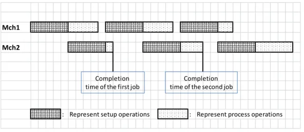
(Shortest Processing Time) gives optimal schedule for total completion time objective on a single machine, sorting jobs in ascending order of their processing times on the second machine gives the optimal schedule for our problem. Figure 3.2. illustrates this case.

Figure 3.2: Example of an Optimal Schedule for the Special Case. Mch1

Mch2

: Represent setup operations : Represent process operations

Completion time of the first job

Completion time of the second job

(24)

15

Chapter 4 Lower Bounds and Heuristic

Solution Mechanisms

In this chapter we first present lower bounds to help assess the quality of heuristic solutions on large instances. Then, to aid in solving larger instances a greedy constructive heuristic is proposed to get an initial feasible solution. Later, we introduce representation and validation of the solutions. Lastly, we describe an already existing Variable Neighborhood Search (VNS) Algorithm, discovered search methods and implementation of VNS to our problem.

4.1 Lower Bounds

In this section we develop several lower bounds to help assess the performance of our heuristics in those instances for which exact solutions cannot be obtained in reasonable computational times.

4.1.1 Lower Bound 1

If we relax the capacity of the first machine by assuming that all the jobs are available for processing on the second machine as early as necessary, then we get a relaxed problem which is a single machine scheduling problem where

(25)

16

minimizing the total completion time in a single machine, lower bound 1 can be obtained by computing:

∑ { }

where ∑ is the optimal total completion time of the problem defined on machine 2 and obtained by the SPT rule based on the total setup time and processing time of each job. Also, { } is added, because it corresponds to

the smallest unavoidable idle time on machine 2.

Since this lower bound mainly considers second machine setup times and processing times, it is expected to gıve good bounds for the instances where setup operations and processing operations on the second machine are much longer than those on the first machine.

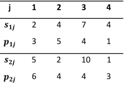
To illustrate this lower bound, consider the following toy problem.

Table 4.1: Data for Toy Problem

j 1 2 3 4 2 4 7 4 3 5 4 1 5 2 10 1 6 4 4 3 We compute j 1 2 3 4 11 6 14 4

By applying the SPT rule, we obtain the job sequence {4,2,1,3}. So,

∑ ( ) ( ) ( ) ( ) Thus,

(26)

17

4.1.2 Lower Bound 2

No two setups can be carried out simultaneously on the single server. The best case is that the server is continuously busy performing setups until the beginning of the processing of the last job on machine 2. Hence lower bound 2 can be obtained by relaxing the problem to a single machine where for all j. Since

completion time is defined as the finishing time of process on second machine, lower bound 2 can be defined as:

∑ ∑

where ∑ is the optimal total completion time of the relaxed single machine problem and obtained by the SPT rule after merging the first machine setup time and the second machine setup time of each job. Also, ∑ is added, because

job is completed when process ends on the second machine.

Since we mainly consider setup times while computing this lower bound, it is expected to produce good bounds for the instances in which, setup times are generally greater than processing times on both machines. We apply this lower bound on the toy problem.

We compute

j 1 2 3 4

7 6 17 5

By applying the SPT rule, we obtain the job sequence {4,2,1,3}. So,

∑ ( ) ( ) ( ) ( )

∑

Thus,

(27)

18

4.1.3 Lower Bound 3

The best case on machine 1 is when there is no idle time. Hence, we relax the capacity of the second machine. Then we get a relaxed problem which is a single machine scheduling problem where for all j. Lower bound 3 can be

obtained by computing:

∑

where ∑ is the optimal total completion time of the problem defined on machine 1 and obtained by the SPT rule based on the total setup time and processing time of each job on machine 1 and is the possible idle times that can occur on the second machine. There are two possible cases that job can be setup on the second machine. In the first case ( ) and starts as soon as finishes on the

first machine. Idle time doesn’t occur on the second machine while starts as

soon as finishes on the first machine. Differently from first case, in the second

case ( ) which causes ( ) unit idle time on the second machine

because can be started on the second machine after is completed. Figure

4.1. illustrates these cases in which, it can be seen that idle time occurs at least ( ) time units for each job. Total completion time objective grows cumulatively hence any idle time for job affects also all the jobs which are processed after . Therefore, we consider small idle times early and large idle times late as much as possible on the schedule. So, jobs are sorted in ascending order of ( ) values and multiplied with ( ) where ( ) gives the order of job j in ascending orders.

This lower bound mainly considers setup times and processing times on the first machine. Hence for the instances that have larger processing and setup operations on the first machine, it is expected to give good bounds. However, effect of the idle times that may be experienced on the second machine is also considered as much as possible. Thus, this lower bound is expected to work well for the instances in which average of setup times and average of processing times are near each other on machines 1 and 2.

(28)

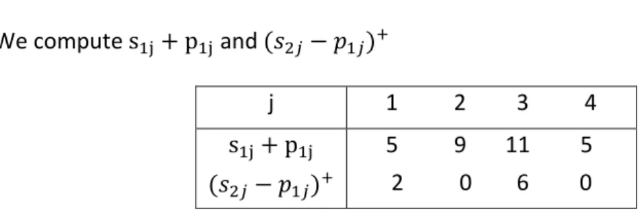
19 Consider the toy problem to illustrate LB 3:

We compute and ( ) j 1 2 3 4 ( ) 5 9 11 5 2 0 6 0

By applying the SPT rule, we obtain the job sequence {4, 1, 2, 3}. So,

∑ ( ) ( ) ( ) ( ) Ascending order of ( ) is . So,

( ) ( ) ( ) ( ) Thus,

Figure 4.1: Possible Idle Times for the LB 3

4.1.4 Lower Bound 4 and Lower Bound 5

These lower bounds are improved versions of lower bound 3. First we transform the problem in to the classical flow shop problem (i.e., one without setups) with the total completion time objective in such a way that the optimum objective function value of the transformed problem will always be smaller than that of the original problem. In order to make this transformation, we redefine the processing time of each job j on machine 1 as where . We then completely

Mch 1

Mch 2

Case 1:

Mch 2

Case 2:

:

[DelayTime=0]

[Delay Time =(

)]

Represent

(29)

20

disregard the setup operations on the second machine and consider only the processing times for . Now the problem is transformed into the

classical problem any lower bound for which will also be a lower bound for our original problem.

After this transformation, we use the lower bound developed by Han Hoogeveen et al. [23]. They formulate the classical two stage flow shop problem as an integer program (IP) using positional completion time variables. They show that solving the linear programming relaxation of their IP model gives a very strong lower bound. We use both their integer programming model and its LP relaxation to obtain lower bounds for our problem. Model is as follows.

∑ ∑ ∑( ) ∑( ) s.t. ∑ ∑ ∑ ∑ ∑ ∑ ∑

where represents the first machine process, represents the second machine process, is the slack variable and is the binary variable, which takes on a value

of 1 if job is assigned to position , and it is 0 otherwise. Constraint (1) is the objective function which tries to minimize total completion time of the jobs. Constraint sets (2) and (3) ensure that only one job can be assigned to one position. Constraint (4) satisfies the machine capacity conditions. Finally, constraint sets (5)

(1) (2) (3) (4) (5) (6)

(30)

21

and (6) give the non-negativity and binary restrictions. By solving this IP model, lower bound 4 can be obtained.

Lower bound 5 is obtained by solving the version of the problem that relaxes the binary constraints to and . Hence for the instances up to 35 jobs

lower bound 5 is not computed as it can never be better than lower bound 4. However, it is not possible to obtain lower bound 4 for the N=50 and N=100 instances in reasonable computational times. Thus, lower bound 5 is computed instead for these instances.

Lower bounds 4 and 5 ignore the single setup server and setup operations on the second machine. They rather focus on only the job processing where processing times on the first machine are adjusted to include also the respective setup times. Since effects of the single setup server and setup times on the second machine are ignored, it is expected to give good bounds for the instances where processing times are generally greater than setup times on both machines.

4.2 Heuristic Solution Mechanisms

In this section we propose a constructive method to obtain an initial solution followed by two versions of a VNS mechanism that are intended to improve this starting solution.

4.2.1 Greedy Constructive Heuristic

This heuristic aims to produce a full schedule by inserting one job at a time, into a partial schedule in a greedy manner. It enforces a permutation schedule in the sense that jobs are processed in the same order on machines 1 and 2. In each step, each unscheduled job is considered as a candidate for the next position. The candidate that increases objective function by the minimum value is selected from the set.

(31)

22

Define as the starting time of the next setup on first machine and as

the finishing time of the last process on second machine for a given partial schedule. The details of the algorithm are as presented in the following.

Algorithm (Greedy Constructive Heuristic)

Step 1. (Initialization)

Select the job with the maximum total completion time on the second machine as the first job in the schedule.

Place

Step 2. (Analysis of Remaining Jobs to be scheduled)

For each job that has not yet been scheduled do the following: Consider that job as the next one in the partial sequence and compute the total completion time of all the jobs scheduled until that point.

Step 3. (Selection of the Next Job in Partial Schedule)

Of all jobs analyzed in Step 2, select the job with the smallest total completion time as the next one in the partial sequence.

Place { { } }

Step 4. (Stopping Criterion)

If STOP. Else, Go to Step 2.

4.2.2 Representation and Validation of Solutions

We represent a solution as an integer array of length , where is the number of jobs. Each entry of the array indicates setup of a job on machines 1 and 2. For any job j, its setup on the first machine is represented as j while that on the second machine is represented as . Since processing has to take place as soon as possible on either machine, we are able to construct the full schedule when the

(32)

23

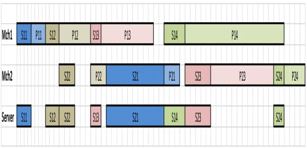
setup sequence on the two machines is known. To illustrate this, consider the following example where =4 and setup order is [1,2,6,3,5,4,7,8]. Figure 4.2 shows a Gantt chart of the solution corresponding to this order.

Figure 4.2: Solution Representation for the Given Example

Note that for each job, first machine operation must be done before second machine operation. Thus, in our solution representation, j must precede for all , for the corresponding solution to be feasible.

4.2.3 Variable Neighborhood Search (VNS)

Large set of tools are (Branch & Bound, IP Formulation etc.) available to solve defined problem exactly, but they may not suffice to solve large instances due to complexity issues. Hence, we present heuristic algorithms to solve larger instances. A common heuristic approach is local search which starts with an initial solution and attempts to improve its objective function value by a sequence of local changes within a given search neighborhood. It usually continues with its search until a local optimum is reached.

In this study, we use a version of this common technique known as Variable Neighborhood Search (VNS) which was originally proposed by Hansen [24]. Instead of stopping at a local optimum point with respect to a given neighborhood, VNS

Mch1

Mch2

Server

S12

P24

P13

P21

S11

S22

S13

S21

S14

S23

S24

S14

P14

S23

P23

S24

S11 P11 S12

P12

S22

P22

S13

S21

(33)

24

searches different neighborhoods of the current incumbent solution. It jumps from this solution to a new one if and only if an improvement has been seen. Hence, it tries to find better local optimum points at each time. If there is not any improvement on the objective function value, then VNS algorithm terminates with the best solution at hand.

A finite set of neighborhood structures denoted with ( )

and the set of solutions in the neighborhood of are denoted with ( ) are defined. VNS algorithm starts with initialization step in which, the set of neighborhood structures , = 1,…., , that will be used in the search are

selected and initial solution is found. Additionally stopping condition should be chosen in this step.

Search mechanism starts from first neighborhood structure, namely . Later a point at random from the neighborhood of ( ( )) is generated. Some local search method is applied to and local optimum is obtained. At this point a decision is made to move or not to this new point. If this local optimum is better than the incumbent, the move decision is made and search is continued with the very beginning of the neighborhood structures, i.e. ( ). Otherwise, the following neighborhood structure is applied. This routine continues until the stopping condition is met.

Greedy constructive heuristic always generates a permutation schedule as an initial solution but the optimum solution may be a non-permutation schedule. Search methods are defined for the aim of also generating non-permutation schedules from a given initial permutation schedule. At this point, we decide to use VNS mechanism for defining a strategy to make crossing operations of search methods between each other with the intent of obtaining better objective values.

4.2.4 Neighborhood Structures

Before describing VNS algorithms which are adapted for our problem, four search methods are presented as neighborhood structures of the VNS algorithm.

(34)

25

As we mentioned before, the solution is represented as an integer array of length , and each entry of the array indicates a setup on either machine 1 or on machine 2. Search strategies are based on change of entries in this array. The crucial point is that, new solution must be feasible in the sense that no job has a setup on the second machine before having one on the first. We use the following neighborhood search structures.

1. Insert Search:

The idea of this method is searching through different orders obtained by inserting jobs to each other’s positions, i.e. changing machine 1 order.

Method starts for the first setup operation on machine 1, i.e. the first entry in solution array which satisfies condition and tries to insert setup operation of job j instead of following setup operations on machine 1 respectively. Inserting one setup operation to a new position in machine 1, affects the second machine setup order. Because of this, after each insert trial for setup operation in machine 1, method searches for possible positions in machine 2 for the subject job. This is required to generate feasible and new solutions. Inserting one job to a new position in machine 1 and searching for possible positions in machine 2 is called a trial. These trials are carried out for each job and machine 1 position pairs in a systematic way. For one job all possible positions in machine 1 are searched then search continues with the next job trials.

If there is an improvement in the objective function value during these trials, meaning that one of the new orders has a lower total completion time, then that new order is set as the main order and method starts from the beginning for the subject order. Otherwise, method keeps going until all possible trials are applied and cannot get any improvement on the objective value.

Since insert method searches for possible positions in machine 2 after inserting one job to machine 1, it allows to scan schedules where the solution is non-permutation. The Insert search method can be summarized as follows.

(35)

26

Algorithm (Insert Search Method)

Algorithm starts with a given initial order. Step 2. (Selection of the first job)

First setup operation on the first machine is selected. Step 3. (Deciding insert or not)

Selected setup operation is attempted to be inserted in each one of the other setup operations positions on the first machine except its own position.

After trying to insert one setup operation instead of another setup operation on the first machine, algorithm places second machine setup operation of the selected job to possible locations: from new position of first machine setup operation in the solution array to 2N. This is a single insert trial for the selected job.

If there is an improvement in the objective function value during this insert trial, insert the selected job, update the order and go to Step 1.

Otherwise apply next insert trial for the selected job by choosing next candidate setup operation on the first machine. After trying all candidate jobs, if there is not any improvement in the objective function, then go to Step 4.

Step 4. (Selection of the next job)

If there is not any improvement on the objective function value after applying all Insert trials for the selected job, then next setup operation on the first machine is selected. And go to Step 3.

When all setup operations in the first machine are selected, then STOP.

For a better understanding, following demonstration is given. Through the demonstration, TCTk represents the total completion time for order k and Xi implies

that job X is processed in machine i. According to our solution representation X2=X1+ . Same terminology will be used through the other search method’s

(36)

27 Given order:

TCT0 - A1 A2 B1 B2 C1 C2

Best Bound =TCT0

Method starts with inserting A1 to the position of B1.

A2 B1 A1 B2 C1 C2

Inserting A1 to the position of B1 violates feasibility.(A2 must come after A1) The

algorithm continues to search possible positions for A2.

TCT1 - B1 A1 A2 B2 C1 C2

TCT2 - B1 A1 B2 A2 C1 C2

TCT3 - B1 A1 B2 C1 A2 C2

TCT4 - B1 A1 B2 C1 C2 A2

If TCTi > Best Bound for i = 1,2,3,4, algorithm moves to inserting A1 to the position of

C1.

A2 B1 B2 C1 A1 C2

Inserting A1 to the position of C1 violates feasibility.(A2 must come after A1) The

algorithm continues to search possible positions for A2.

TCT5 - B1 B2 C1 A1 A2 C2

TCT6 - B1 B2 C1 A1 C2 A2

(37)

28

B1 A1 A2 B2 C1 C2

Inserting B1 to the position of A1 does not violate feasibility. As the algorithm

continues to search possible positions for B2, this order will be one of the choices.

TCT7 - B1 B2 A1 A2 C1 C2 TCT8 - B1 A1 B2 A2 C1 C2 . . . TCT9 - B1 A1 A2 C1 C2 B2

The algorithm continues in this manner until all possible trials are carried out or a new order with a better total completion time is found. Let’s say order with TCT9

has a better bound i.e TCT9 < Best Bound, then the algorithm starts from the

beginning for order 9 and Best Bound is equalized to TCT9.

B1 A1 A2 C1 C2 B2

B1 will be inserted to the position of A1

A1 B1 A2 C1 C2 B2

Inserting B1 to the position of A1 does not violate feasibility. As the algorithm

continues to search possible positions for B2, this order will be one of the choices.

TCT10 - A1 B1 B2 A2 C1 C2 TCT11- A1 B1 A2 B2 C1 C2 . . . TCT12 - A1 B1 A2 C1 C2 B2

(38)

29

2. Pairwise Interchange Search:

Basic principal of pairwise interchange method is switching two jobs entirely both in machine one and machine two orders. The method searches for new orders according to the order of machine 1. Method starts with the first setup operation pairs on machines 1 and 2, i.e. the first and second entries in solution array which satisfy condition. After the two jobs are chosen to be interchanged, then the corresponding second machine orders are also switched. This is done in order to preserve feasibility.

In order to avoid searching same orders, each job is tried to be switched respectively with the jobs that comes after it. The procedure continues until a new order with a better solution is obtained or all allowed interchanging operations are applied. In former case, method starts from the beginning for with the new order as the initial order. Otherwise method terminates with the current best solution and the order. The pairwise interchange search method can be summarized as follows.

Algorithm (Pairwise Interchange Search Method)

First setup operation on the first machine is selected. Step 3. (Deciding switch or not)

Selected setup operation is switched with following setup operation on the first machine, and second machine setup operations of the affected jobs are also switched simultaneously. This is a single pairwise interchange trial.

If there is an improvement on the objective function value for the trial, switch the selected job pairs, update the order and go to Step 1.

Else, apply next pairwise interchange trial for the selected setup operation by choosing next setup operation on the first machine.

(39)

30 Step 4. (Selection of the next job)

If there is not any improvement in the objective function value after applying all pairwise interchange trials for the selected job, then the next setup operation on the first machine is selected. And go to Step 3.

When all setup operations in the first machine are selected, then STOP.

Similar to insert method, for a better understanding, following demonstration is given.

Given order:

TCT0 - A1 A2 B1 B2 C1 C2

Best Solution =TCT0

Method starts with switching job A with job B.

B1 A2 A1 B2 C1 C2 - Switching jobs in machine 1 order.

B1 B2 A1 A2 C1 C2 - Switching jobs in machine 2 order.

This is the new feasible order with objective value TCT1 to be checked with current

best solution. If TCT1 > Best Solution, then job A is switched with job C.

C1 A2 B1 B2 A1 C2 - Switching jobs in machine 1 order.

C1 C2 B1 B2 A1 A2 - Switching jobs in machine 2 order.

best solution. If TCT2 > Best Solution, then job B is switched with job C not job A.

A1 A2 C1 B2 B1 C2 - Switching jobs in machine 1 order.

A1 A2 C1 C2 B1 B2 - Switching jobs in machine 2 order.

(40)

31

other than C that comes after B and there is no job that comes after C. However if TCT3 < Best Solution, then the algorithm starts all over again for this new order 3.

First switch will be between A and C.

3. Second Machine Move Search:

According to our problem definition, each job must be setup in machine 1 before setup in machine 2. However there is no constraint for non-permutation, setup operations on the second machine may be done in any order after from its first machine setup operation.

Second machine move method starts with a given feasible order. Therefore, using the fact above, moving each second machine setup operation to the right starting from its own position to end of order does not violates feasibility but generates new feasible solutions for our problem. The second machine move search method can be summarized as follows.

Algorithm (Second Machine Move Search Method)

First setup operation on the second machine is selected. Step 3. (Shifting selected setup operations to the right)

Selected setup operation is shifted right at each trial until to the position 2N in the solution array.

If there is an improvement in the objective function value for the trial; shift selected setup operation to this position, update order and go to Step 1.

Step 4. (Selection of the next job)

If there is not any improvement in the objective function value at the end of any of the trials for the selected job, then next setup operation on the second machine is selected. And go to Step 3.

(41)

32

Method starts with first setup operation on machine 2 i.e., the first entry in the solution array that satisfies . Then it continues for all the second machine setup operations. This procedure continues until all allowed combinations are searched or a new order with a better objective value is found. If a better solution is found, method starts all over again from this new order.

Given order:

TCT0 - A1 A2 B1 B2 C1 C2

Best Solution =TCT0

-Method starts with moving A2 to the right by one unit.

TCT1 - A1 B1 A2 B2 C1 C2

This is a new feasible order with objective value TCT1 to be checked with current

best solution. If TCTi > Best Solution for i = 2, 3, 4, then job A2 continues to move to

the right until 2N.

TCT2 - A1 B1 B2 A2 C1 C2

TCT3 - A1 B1 B2 C1 A2 C2

TCT4 - A1 B1 B2 C1 C2 A2

If a better solution is not found, method moves to second setup in machine 2.

-Moving B2 to the right by one unit.

(42)

33

The algorithm continues in this manner until all combinations are searched or a better solution is found. Let’s say TCT5 < Best Solution, then order 5 is the new main

order and the method starts from the beginning for order 5 by moving A2 to the

right.

4. First Machine Move Search:

First machine move method uses the same logic with the second machine move method. Method starts with first setup operation in machine 1 according to the given solution i.e., first entry in the solution array that satisfies . For each job all possible positions are searched from its position in solution array to zero index. Then it continues for all the first machine setup operations. This routine continues until all allowed combinations are searched or a new order with a better objective value is found. If a better solution is found, method starts all over again from this new order. The first machine move search method can be summarized as follows.

Algorithm (First Machine Move Search Method)

Second setup operation on the first machine is selected. Step 3. (Shifting selected setup operations to the left)

Selected setup operation is shifted left at each trial until to the (position 0) in the solution array.

If there is an improvement in the objective function value for the trial; shift the selected setup operation to this position, update the order and go to Step 1. Step 4. (Selection of the next job)

If there is not any improvement in the objective function value at the end of all trials for the selected job, then next setup operation on the first machine is selected. And go to Step 3.

(43)

34 Given order:

TCT0 - A1 A2 B1 B2 C1 C2

Best Solution =TCT0

-Method would try to move A1 to the left. However since it is the first job of the

order, method will move to second job in machine 1 which is B1.

TCT1 - A1 B1 A2 B2 C1 C2

This is a new feasible order with objective value TCT1 to be checked with current

best solution. If TCT1 > Best Solution, then job B1 continues to move to the left until

index 0.

TCT2 - B1 A1 A2 B2 C1 C2

If a better solution is not found, method moves to the third job processed in machine 1, C1.

-Moving C1 to the left by one unit.

TCT3 - A1 A2 B1 C1 B2 C2

TCT4 - A1 A2 C1 B1 B2 C2

Method continues to move C1 until a better solution is found or C1 is tried at each

position from its original position to 0. Let’s say order 4 is a better solution. Then it becomes the main order and method starts all over again for order 4, by again trying to move A1 to the left then by moving second job C1 to the left unit by unit.

(44)

35

4.2.5 VNS 1 Algorithm

The VNS 1 algorithm takes in the initial solution obtained from the constructive heuristic and attempts to improve it by searching the Insert, Pairwise Interchange, Second Machine Move and First Machine Move neighborhood structures. When the local optimum at a given neighborhood results in an improvement in the objective function value of the initial solution fed into that neighborhood in the current iteration, the search mechanism goes back to the Insert neighborhood and starts a new iteration with the current best solution found up to that point. VNS 1 algorithm terminates only, if there isn’t any improvement on the objective value at the end of last search method.

Initial experimentation shows that the order in which different neighborhoods are searched has an effect on solution quality. Nonetheless, there is no evidence that indicates that any particular order is better than the other. Thus we make a judgment call and first search the insert and pairwise interchange neighborhoods that are of larger sizes than the other two. Then second machine move and first machine move neighborhoods are searched respectively. Since we have no clear direction on whether insert should precede or succeed interchange, we try both resulting in cases 1 and 2, respectively. Hence we compute solution of both cases and accept solution which has the minimum objective value. During this thesis, VNS algorithms are described on case 1 in which insert method is applied first. For the second case, everything is the same except that order of insert search and pairwise search is exchanged. The details of the algorithm are as presented in the following.

Algorithm (Variable Neighborhood Search 1)

Apply Greedy Constructive Heuristic and find an initial order. Best Solution = Initial Solution

Best Order = Initial Order. Step 2. (Insert Search Method)

Execute insert search method for the best order. If Insert Solution Best Solution

(45)

36 Best Solution = Insert Solution Best Order = Insert Order Go to the Step 3.

Step 3. (Pairwise interchange Search Method)

Execute pairwise interchange search method for best order. If Pairwise Solution Best Solution

Best Solution = Pairwise Solution Best Order = Pairwise Order Go to the Step 2.

Else, Go to the Step 4.

Step 4. (Second Machine Move Search Method)

Execute second machine move search method for best order. If Second Machine Move Solution Best Solution

Best Solution = Second Machine Move Solution Best Order = Second Machine Move Order Go to the Step 2.

Else, Go to the Step 5.

Step 5. (First Machine Move Search Method)

Execute first machine move search method for best order. If First Machine Move Solution Best Solution

Best Solution = First Machine Move Solution Best Order = First Machine Move Order Go to the Step 2.

Else, STOP and RETURN Best Solution and Best Order.

(46)

37

(47)

38

4.2.6 VNS 2 Algorithm

The motivation behind the VNS 2 algorithm is that solving VNS 1 may still be computationally expensive for larger problems. In VNS-1 algorithm, search methods work recursively in the sense that the search begins a new each time local optimum solution is found. For any search method, if a better order is found then search mechanism starts from scratch for this order. At this point, we decide to limit number of search trials of each candidate job in search methods. Since, each job should have a chance to be tried for all possible positions; we limit number of search trials with the number of jobs.

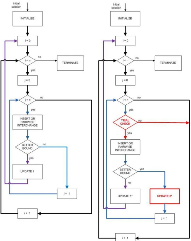
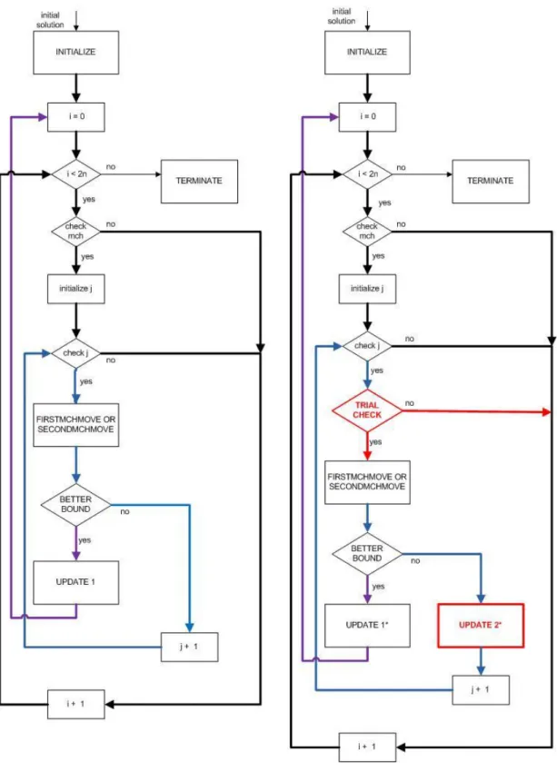
For a better understanding a flow chart is presented for insert and pairwise interchange search methods in Figure 4.4 and another flow chart is presented for first machine move and second machine move methods in Figure 4.5. Working principles of the insert and pairwise interchange search methods are similar. Hence they are explained through the same flow chart. This is also the case for First Machine Move and Second Machine Move methods hence they are also explained on the same flow chart. As clearly seen on flow charts, additionally to VNS 1 algorithm, trial check step is added to VNS 2 algorithm for each search method.

(48)

39

(49)

40

Figure 4.5: Flow Chart of First Machine Move/Second Machine Move Methods for VNS 1 and VNS 2

Minimazing the total completion time in a two stage flow shop with a single setup server

MINIMIZING THE TOTAL COMPLETION TIME IN A TWO

STAGE FLOW SHOP WITH A SINGLE SETUP SERVER

A THESİS

SUBMITTED TO THE DEPARTMENT OF INDUSTRIAL ENGINEERING

AND THE GRADUATE SCHOOL OF ENGINEERING AND SCIENCE

OF BILKENT UNIVERSITY

IN PARTIAL FULFILLMENT OF THE REQUIREMENTS

FOR THE DEGREE OF

MASTER OF SCIENCE

By

Muhammet KOLAY

July, 2012

ABSTRACT

MINIMIZING THE TOTAL COMPLETION TIME IN A TWO STAGE FLOW

SHOP WITH A SINGLE SETUP SERVER

ÖZET

TEK SUNUCULU İKİ AŞAMALI SERİ AKIŞDA

TOPLAM TAMAMLANMA ZAMANINI EN AZLAMAK

Acknowledgement

Contents

List of Figures

List of Tables

Chapter 1

Introduction

Chapter 2

Literature Review

Chapter 3

Problem Definition

3.1 Problem Definition

Time

Mch1

3

Mch2

Server

2

1

4

3

4

2

1

3.2 The Mixed Integer Programming Model

3.2.1 Parameters

3.2.2 Variables

3.2.3 MIP Model

3.3 Polynomial-Time Solvable Case

Chapter 4

Lower Bounds and Heuristic

Solution Mechanisms

4.1 Lower Bounds

4.1.1 Lower Bound 1

4.1.2 Lower Bound 2

4.1.3 Lower Bound 3

4.1.4 Lower Bound 4 and Lower Bound 5

Mch 1

Mch 2

Case 1:

Mch 2

Case 2:

:

:

[DelayTime=0]

[Delay Time =(

)]

Represent

Represent

4.2 Heuristic Solution Mechanisms

4.2.1 Greedy Constructive Heuristic

4.2.2 Representation and Validation of Solutions

4.2.3 Variable Neighborhood Search (VNS)

Mch1

Mch2

Server

S12

P24

P13

P21

S11

S22