1. Introduction
The effect of exchange rate fluctuations on macroeconomic performance is a heavily researched topic. The conventional Mundell-Fleming model clearly depicts the relationship between the exchange rate and an economy’s output level. According to the conventional model, expansionary monetary policy reduces the interest rate, which leads to a depreciation of a country’s exchange rate. Hence, the depreciation of currency stimulates the aggregate demand by boosting exports and discouraging imports in favor of domestically produced goods. Many studies provide empirical evidence for the depreciation (or devaluation) of a national currency stimulating economic activity. For example, Agénor (1991) analyzed the effect of real exchange rate changes on output in a rational expectations macro-model with imported intermediate goods. Using the data for a group of 23 developing countries over the period from 1978-87, he found that an unanticipated real exchange rate depreciation boosts the output growth. The study by Hoffmaister and Végh (1996) was the first attempt to provide empirical evidence on the recession-now-recession-later hypothesis for the Uruguayan economy using a vector-autoregression model (VAR) under the exchange rate-based disinflation program. They found that a permanent depreciation in the exchange rate leads to a long-lasting positive effect on output. Santaella and Vela (1996) reached similar results in a VAR for the Mexican economy. However, the positive effect of nominal exchange rate depreciation on output wasreversed after three years (Connolly 1983 and Arize 1994). Contrary to conventional wisdom, there is a substantial literature to show that exchange rate devaluation might have contractionary effects on economic activities. According to Krugman and Taylor (1978) and Cooper (1971), pioneers of the “contractionary
devaluation” argument, the outcome of exchange rate devaluations might be contractionary
by focusing on the adverse income effects of the devaluation. Nominal rigidities, external debt and foreign-currency-denominated liabilities, supply-side-related problems, capital account problems, and associated economic policies in the economy are some of the various channels that explain the contractionary effects of devaluations (see Kamin and Rogers 2000, and Berument and Pasaogullar 2003 for the details). Many empirical studies such as Kamin (1988), Edwards (1989), Agoner (1991), and Morley (1992) are among those that support the argument of the “contractionary effect of exchange rate depreciation on output and/or economic growth.” Copelman and Werner (1996) empirically analyzed the relationship among the output, real exchange rate, rate of depreciation of the nominal exchange rate, real interest rate, and a measure of real credit or real money balances variables in a VAR model for the Mexican data. They found that positive shocks to the rate of exchange rate depreciation significantly reduce credit availability and depress the level of output. The study by Kamin and Rogers (2000) yielded similar results with a five-variable VAR --- output, the real exchange rate, inflation, and the U.S. interest rate --- applied to Mexico. They found that although the variation of output was explained mostly by its own innovations, the response of output to a permanent depreciation was permanent and negative.
The fluctuations of exchange rate movement can be attributable to different shocks such as real (e.g., productivity, labor supply or structural reforms), and/or policy induced/demand shocks (e.g., fiscal and monetary policies). It is generally accepted that an expansionary monetary policy shock leads to currency depreciation, which generates an expansionary effect through aggregate demand by lowering interest rates. On the other hand, it seems likely that fluctuations in the exchange rate are related to the shifts in portfolio preferences of economic agents to guard themselves from an adverse future development. In the presence of financial market uncertainty, such as the expectation of future inflation or political developments, private investors (economic agents) may respond to this uncertainty by shifting out of domestic currency dominated portfolios to foreign currency dominated assets.
The significant shifts in portfolio preferences may lead to depreciation in the domestic currency, which may result in an adverse effect on price levels and a weakening of the confidence level of economic agents. Therefore, a significant shift in portfolio preferences generates a contractionary effect on the economy through aggregate demand. Moreover, the source of exchange rate movements may have different effects on macroeconomic performance. This paper assesses the effect of exchange rate depreciation on macroeconomic performance due to either expansionary monetary policy or portfolio preference changes of economic agents by using quarterly data from Turkey for the period from 1987:Q1 to 2008:Q3.
The Turkish economy offers several unique structural economic characters in the context of assessing the effect of exchange rate movements on macroeconomic performance. First of all, Turkey is a small-open economy with a historically high level of inflation. Turkey has experienced a high and persistent level of inflation for more than three decades without running into hyperinflation. Therefore, the relationships between the money aggregates and macroeconomic variables are more visible because of the high variability of monetary policy changes and the high degree of price level variability (Berument 2007, and Kara et al. 2007). The high variability of these series decreases the chance of a Type II error- error made when the incorrect null hypothesis is not rejected. Therefore, it is easier to find economic relationships in the Turkish data that could not be observed from any other country’s data set. In addition, Turkey has never adopted the fixed exchange rate regime, so Turkish monetary policy is not endogenous. This allows us to assess the role of monetary policy on the exchange rate (see Berument et al. 2011 for details). Finally, Turkey has relatively well developed and liberal financial markets; in particular, money, foreign exchange, and bond markets operate without heavy regulation. The fluctuations of economic variables are due to viable financial markets rather than the initiations of a few speculators/manipulators.
The contribution of this paper to the existing literature is two fold. First, we employ Uhlig’s (2005) sign restriction approach to identify the source of exchange rate movements as either a monetary policy shock or a portfolio choice shock. Second, this study assesses how these two shocks affect the overall macroeconomic performance of the Turkish economy. The findings suggest that: (i) effects of exchange rate movement on macroeconomic activities are expansionary if the exchange rate depreciation stems from an expansionary monetary policy; (ii) if the currency depreciation stems from a portfolio choice allocation, then this effect is contractionary.
The following section introduces the methodology. Both data and empirical evidence are discussed in sections 3 and 4, respectively. The last section is for the conclusion.
2. Methodology
This paper employs VAR methodology to assess the different effects of exchange rate movements that stem from different sources on macroeconomic performance. In order to distinguish the differential effect of exchange rate movements, Uhlig’s (2005) sign restriction methodology is employed. To describe the relationship between structural VAR’s one-step-ahead prediction errors and structural macroeconomic shocks, we use a VAR in a reduced form 1 1 1 1 () ... − + + + = + t + + k t k + t t ct BY B Y u Y (1)
where Yt+1 is an (m × 1) vector containing each of the m variables included in the VAR model, Bj are coefficient matrices of size m ×m, c(t) contains constant and possible time
trend term, and ut+1 is the one-step ahead prediction error with variance-covariance matrix ∑ = ′+ + ] [ut 1 tu 1 E .
The usual structural VAR approach assumes that the error terms ut+1 are related to the structural macroeconomic shocks,vt+1, via matrix A such that
1 1 + + = t t Av u , E vt vt′ =Im + + ] [ 1 1 (2)
In this study, since two different exchange rate shocks are identified, any type of shock to an exchange rate is estimated by vER. The prediction errors in the VAR model are characterized as being decomposed in the following way
1 1 1 ~ 1 ~ + + + = + ′ t ER t t Av Av u (3)
where A1 is the ith column of the matrix A, A
~′
is the (m× (m - 1)) matrix of the remaining columns of A and v~ is the ((m - 1)×1) matrix of the remaining unidentified fundamental shocks. Therefore, all the identified shocks can have an instantaneous effect on all variables. Where, the jth column of A represents the immediate impact on all variable of the jth innovation. A A A ] v v [ AE ] u u [ E t t′ = t t′ ′= ′ = ∑ , A =A~Q (4)
In order to achieve identification, m(m-1)/2 degrees of freedom in specifying A are needed. In the study by Uhlig (2005), Q is an orthogonal and A~ is the Cholesky decomposition of the estimated matrix of covariance residuals Σˆ (A~A~′=∑). Thus, determining the free elements in A can be conveniently transformed into the problem of choosing elements in an orthogonal set. The impulse vector a is a column of the matrix A. In our study, a is an impulse vector for any type of exchange rate shock, if and only if there is an m-dimensional vector
α
of unit length so thatα
A
a = ~ (5)
where α is a column of the matrix Q. Given an impulse vector a, it is easy to calculate the appropriate impulse response in the following way. Let ri(k)be the impulse response at period k to the ith shock obtained by the A~, so the impulse response for a at horizon k is given as follows
∑
= = m i i i a(k) r (k) r 1 α (6)For any type of shock to the exchange rate, the methodology tests whethera∈A(Bˆ,Σˆ,K) is
an exchange rate shock, by checking the appropriate sign restrictions on the impulse responses for all relevant horizon periods k.
Uhlig’s (2005) sign-restriction methodology is an agnostic identification procedure, which imposes sign-restrictions on the impulse responses of selected variables for a certain period following the shock. The brief summary of Uhlig’s (2005) pure-sign restriction approach can be given as follows
(1) Take n1 draws from the VAR posterior Normal-Wishart distribution and, for each of these draws, n2 draws a from independent uniform prior.
(2) Construct the impulse vector
(3) For each impulse, calculate n1 x n2 impulse responses at horizon k=0,…,K 1 . (4) Check whether the impulse response functions satisfy the sign restrictions and keep it, if the impulse response satisfies the sign restrictions, otherwise discard it.
(5) Collect the n3 impulse responses for each shock using the loss function and plot their 16th, 50th and 84th percentiles 2
.
This pure-sign restriction approach has several advantages. First, to identify a shock (in this study, any type of exchange rate shock: a monetary policy shock or portfolio choice
1 We take n
1=n2=200, so there are 40000 draws in total in this study.
2 We take n
shock), the signs of the impulse responses of a shock are restricted based upon received opinions on what these signs should be for a period of time. Second, since a shock is identified by using impulse responses for several periods following the shock, a wide range of shocks can be captured. Third, impulse responses are drawing from the posterior distribution of the reduced form VAR covariance matrix and coefficients, and from the set of structural matrices consistent with the assumed sign restrictions. So the pure-sign restriction performs relatively well compared to the identification methods based on contemporaneous zero restrictions (Mountford 2005).
3. Data
In order to assess the different effects of exchange rate movements on economic performance, in this study, we gather data from Turkey. We use quarterly data of the interbank interest rate as our measure of the interest rate, M1 plus REPO3 as money supply, Turkish Lira (TL) value of US dollar as an exchange rate, GDP deflator as prices, and GDP as income. The quarterly data are obtained from the Central Bank of the Republic of Turkey (CBRT) Electronic Data Delivery System and the estimation period is from1987:Q1 to 2008:Q3.
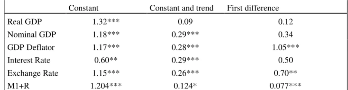
All data are expressed in the logarithmic form except the interest rate. Prior to selecting the specification of the variables in the VAR system, one needs to examine the time series properties of the variables. An Augmented Dickey Fuller (ADF, 1981), Phillips-Perron (PP, 1989) and Kwiatkowski, Phillips, Schmidt and Shin (KPSS, 1992) unit root tests are performed. Table I and II present the results for seasonally unadjusted data and seasonally adjusted data, respectively.
Table I
The Results of ADF, PP and KPSS Unit Root Test
ADF
Constant Constant and trend First difference
Laga Laga Laga
Real GDP 8 -0.740 8 -2.640 7 -3.074** Nominal GDP 8 -2.47 8 -0.397 7 0.47 GDP Deflator 4 -2.18 4 -0.10 3 -1.13 Interest Rate 2 -2.52 0 -4.49*** 1 -10.33*** Exchange Rate 1 -2.50 1 0.30 0 -5.95*** M1+R 0 -0.650 0 -2.571 0 -10.089*** PP
Constant Constant and trend First difference
Real GDP -4.98*** -8.96*** -14.31*** Nominal GDP -3.26** 1.20 -9.18*** GDP Deflator -4.41*** 1.49 -8.90*** Interest Rate -3.69*** -4.33*** -21.33*** Exchange Rate -2.56 0.61 -6.01*** M1+R -0.678 -2.534 -10.135*** KPSS 3
The reasons for including REPO in money aggregates: this money aggregate is liquid because most of the repo transactions are overnight, and agents prefer to repo their savings rather than to open deposit accounts since the repo rates are considerably higher during the period that we consider.
Constant Constant and trend First difference Real GDP 1.32*** 0.09 0.12 Nominal GDP 1.18*** 0.29*** 0.34 GDP Deflator 1.17*** 0.28*** 1.05*** Interest Rate 0.60** 0.29*** 0.50 Exchange Rate 1.15*** 0.26*** 0.70** M1+R 1.204*** 0.124* 0.077***
Note: * significant at the 10% level. ** significant at the 5% level. *** significant at the 1% level.
a the lag order is determined by Shwarz Bayesian Criteria
Table II
Unit Root Test Results for Seasonally Adjusted Data
ADF
Constant Constant and trend First difference
laga laga laga
Real GDP 0 -1.21 0 -2.64 3 -6.14***
Nominal GDP 9 -2.44 2 1.49 5 -0.08
PP
Constant Constant and trend First difference
Real GDP -1.21 -2.89 -9.18***
Nominal GDP -4.16** 2.98 -3.11**
KPSS
Constant Constant and trend First difference
Real GDP 1.17*** 0.07 0.07
Nominal GDP 1.18*** 0.28*** 1.05***
Note: * significant at the 10% level. ** significant at the 5% level. *** significant at the 1% level.
a the lag order is determined by Shwarz Bayesian Criteria
These two tables suggest that all variables have a unit root. This paper uses the multivariate cointegration technique proposed by Johansen and Juselius (1990) in order to test whether there is a long-run relationship among all variables.Table III reports the results of maximum eigenvalue and trace tests statistics.
Table III
Johansen’s Cointegration Tests
The number of cointegrating relations Trace statistic Max-Eigen statistic
None* ( 0.000) 218.638 (0.0000) 141.317
At most 1* (0.000) 77.321 (0.0001) 57.589
At most 2 ( 0.441) 19.731 (0.478) 12.715
At most 3 (0.575) 7.016 ( 0.623) 5.923
At most 4 (0.295) 1.092 (0.295) 1.092
Note: 1. While maximum lag length is 4, the order level VAR is estimated as 1 using Schwarz criteria. 2. Values in parentheses are MacKinnon-Haug-Michelis (1999) p-values. Both trace and max- eigenvalue tests indicate 1 cointegrating equation at the 10% level.
The trace test and maximum eigenvalue tests show that the null hypothesis of r = 0 against the alternative r = 1 is rejected at the 95 percent level. This suggests that there is at least one cointegrating relationship; therefore, the estimation of the VAR in (log) levels provides consistent estimates (Sims et al. 1990, and Lütkepohl and Reimers 1992). Moreover, in the Bayesian VAR methodology of Sims and Uhlig (1991) and Uhlig (2005), the parameters of VAR in level are estimated. This methodology is robust in the presence of non-stationarity, and although it does not impose any cointegrating long-run relationship between the variables and it does not rule out their existence either (Mountford 2005). Therefore, the variables in VAR are used in levels for this study.
4. Empirical Evidence
The impulse responses are reported in Figure 1a-1b and Figure 2a-2b. The confidence intervals are generated by using the Bayesian approach of Sims and Zha (1998) and Uhlig (1994), by taking draws from the posterior distribution, and identifying the exchange rate shocks for each case (i.e. a monetary policy shock or portfolio choice shock). The middle lines in the figures represent the impulse responses. One standard deviation confidence interval around the reponse line are shown in blue. If the confidence interval includes the horizontal line for value of zero, the null hypothesis that there is no effect cannot be rejected. Figure 1a
Currency Depreciation Due to Expansionary Monetary Policy
Impulse Responses for ex
0 1 2 3 4 5 6 7 8 9 0.00 0.50 1.00 1.50 2.00 2.50 3.00 3.50 4.00 4.50
Impulse Responses for Interest Rate
0 1 2 3 4 5 6 7 8 9 -10.00 -8.00 -6.00 -4.00 -2.00 0.00 2.00
Impulse Responses for Income
0 1 2 3 4 5 6 7 8 9 -2.00 -1.50 -1.00 -0.50 0.00 0.50 1.00 1.50 2.00
Impulse Responses for p
0 1 2 3 4 5 6 7 8 9 -0.01 -0.01 -0.00 0.00 0.01 0.01 0.02 0.02
Impulse Responses for m
0 1 2 3 4 5 6 7 8 9 -4.00 -2.00 0.00 2.00 4.00 6.00 8.00
Figure 1a contains impulse responses of exchange rate, price level, interest rate, money aggregate, and real income to a positive exchange rate shock due to an expansionary monetary policy stance. Our sign restrictions for the currency depreciation due to a monetary policy shock are given in Table IV.
Table IV
Identifying Sign Restrictions for Depreciation due to Monetary Policy
Shocks Exchange rate Interest Rate GDP Price M1+R
Depreciation due to monetary policy + - NR NR +
Note: The table shows the sign restrictions on the impulse responses for each identified shock.‘+’ means that the impulse response of the variable in question is restricted to be positive for two quarters following the shock, including the quarter of impact. Likewise, ‘-’ indicates a negative response. A ‘NR’ indicates that no restrictions have been imposed.
We assume that the exchange rate shock stemming from expansionary monetary policy does not lead to a decrease in the exchange rate, a decrease in the money aggregate, and increase in the interest rate in the first two quarters following the shock. Our results indicate that the impulse response of exchange rate increases after a shock and this effect is persistent and statistically significant for the ten periods that we considered. Second, the price level is affected positively at the beginning and after the fourth quarter this effect converges to zero. However, this effect is not statistically significant. Third, the effect of interest rate increases through the first 5 quarters and then this effect dies out. The money aggregate is signed as expected and is statistically significant for almost three quarters, after which decays and converges to zero. Finally, output increases but the effect is statistically insignificant. Figure 1b
Currency Depreciation Due to Portfolio Changes
Impulse Responses for ex
0 1 2 3 4 5 6 7 8 9 -0.50 0.00 0.50 1.00 1.50 2.00 2.50 3.00 3.50 4.00
Impulse Responses for Interest Rate
0 1 2 3 4 5 6 7 8 9 -1.00 0.00 1.00 2.00 3.00 4.00 5.00 6.00 7.00
Impulse Responses for Income
0 1 2 3 4 5 6 7 8 9 -3.00 -2.50 -2.00 -1.50 -1.00 -0.50 0.00 0.50 1.00
Impulse Responses for p
0 1 2 3 4 5 6 7 8 9 -0.04 -0.03 -0.03 -0.02 -0.01 -0.01 -0.00 0.00 0.01 0.01
Impulse Responses for m
0 1 2 3 4 5 6 7 8 9 -7.00 -6.00 -5.00 -4.00 -3.00 -2.00 -1.00 0.00
Figure 1b presents the results of the impulse responses for the exchange rate, price level, interest rate, money aggregate, and real income to a positive exchange rate shock due to a non-monetary shock (portfolio preferences). Our sign restrictions for an exchange rate shock stemming from portfolio preferences are given in Table V.
Table V
Identifying Sign Restrictions for Depreciation due to Portfolio Changes
Shocks Exchange rate Interest Rate GDP Price M1+R
Depreciation due to portfolio changes + + NR NR _ Note: The table shows the sign restrictions on the impulse responses for each identified shock.‘+’ means that the impulse response of the variable in question is restricted to be positive for two quarters following the shock, including the quarter of impact. Likewise, ‘-’ indicates a negative response. A ‘NR’ indicates that no
restrictions have been imposed.
The responses of exchange rate and interest rate have been restricted not to be negative, and the money aggregate not to be positive for the first two quarters. During the financial stress, the demand for foreign exchange increases, which may be accompanied by the selling Treasury bills (or bonds) and the liquidation of bank deposits. Our study demonstrates that the effect of a depreciation shock to the exchange rate is positive, persistent and statistically significant until the fifth quarter. In general, the price level increase is accompanied by a currency depreciation. However, this study finds that the price level reacts negatively to the
shock, but it is statistically insignificant. In addition, the response of the interest rate is positive and significant for the first three periods, and then this effect becomes statistically insignificant. However, the decrease in the money aggregate is statistically significant for all periods. Finally, the negative income response to exchange rate shock is statistically insignificant.
Figure 2a
Currency Depreciation Due to Expansionary Monetary Policy
Impulse Responses for ex
0 1 2 3 4 5 6 7 8 9 -1.00 0.00 1.00 2.00 3.00 4.00 5.00
Impulse Responses for Interest Rate
0 1 2 3 4 5 6 7 8 9 -10.00 -8.00 -6.00 -4.00 -2.00 0.00 2.00
Impulse Responses for Income
0 1 2 3 4 5 6 7 8 9 -1.50 -1.00 -0.50 0.00 0.50 1.00 1.50 2.00 2.50
Impulse Responses for p
0 1 2 3 4 5 6 7 8 9 -0.01 0.00 0.01 0.01 0.01 0.02 0.03 0.03 0.04 0.04
Impulse Responses for m
0 1 2 3 4 5 6 7 8 9 0.00 1.00 2.00 3.00 4.00 5.00 6.00 7.00 8.00 Figure 2b
Currency Depreciation Due to Portfolio Changes
Impulse Responses for ex
0 1 2 3 4 5 6 7 8 9 -1.00 0.00 1.00 2.00 3.00 4.00 5.00
Impulse Responses for Interest Rate
0 1 2 3 4 5 6 7 8 9 -1.00 0.00 1.00 2.00 3.00 4.00 5.00 6.00 7.00 8.00
Impulse Responses for Income
0 1 2 3 4 5 6 7 8 9 -2.50 -2.00 -1.50 -1.00 -0.50 0.00 0.50 1.00
Impulse Responses for p
0 1 2 3 4 5 6 7 8 9 -0.04 -0.04 -0.03 -0.03 -0.02 -0.01 -0.01 -0.00 0.00 0.01
Impulse Responses for m
0 1 2 3 4 5 6 7 8 9 -9.00 -8.00 -7.00 -6.00 -5.00 -4.00 -3.00 -2.00 -1.00
The Turkish economy went through a major structural change after 1994 (see Berument, 2007). To check the robustness of our findings with respect to this major structural change, we re-estimate our benchmark VAR model with the subsample covering the period after 1994 era to 2008:Q3. The corresponding impulse responses of our sub-sample results are reported in Figures 2a and 2b. The findings are very similar compared with the full-sample results of our benchmark specification. However, we should mention the two minor differences arising from the sample selection. First, the effect of an exchange rate shock on macroeconomic variables becomes more persistent. For example, the effect of exchange rate depreciation on output is now statistically significant for 9 periods for the post 1994 era, but this effect was significant only for 1 period for the full-sample specification. In addition, the negative increase in the money aggregate is statistically significant for all periods for two types of depreciation. Overall, we can conlude that our findings are not senvitive to the sample
selection for identfying the effects of the monetary and non-monetary shocks on the macroeconomic performance of the Turkish economy.
5. Conclusion
This paper assesses the effect of positive exchange innovation on the macroeconomic performance of the Turkish economy. By using Uhlig’s sign restriction approach, the study identifies the source of exchange rate movements as an either monetary policy shock or a portfolio choice shock. The finding suggests that the effects of exchange rate movements on macroeconomic variables are different depending upon the source of the shock to the exchange rate. If currency depreciation stemming from an expansionary monetary policy shock is associated with a lower interest rate and higher liquidity, then the effect of currency depreciation on the economy is expansionary. On the other hand, if the currency depreciation stemming from portfolio choice allocation isassociated with lower output and liquidity, then the effect of exchange rate deprecation on the economy is contractionary.
References
Agenor, P.R. (1991) “Output, Devaluation, and the Real Exchange Rate in Developing Countries” Weltwirtschaftliches Archive, 127, 18–41.
Arize, A.C. (1994) “Cointergratio Test of a Long-Run Rleation Between in Real Efective Exchange Rate and the Trade Balance” International Economic Journal, 8(3), 1-9. Berument, H. (2007) “Measuring Monetary Policy for a Small Open Economy: Turkey”,
Journal of Macroeconomics, 29: 411-430.
Berument H and M. Pasaogullari (2003) “Effects of the Real Exchange Rate on Output and Inflation: Evidence from Turkey” Developing Economies, 41, 401-435.
Berument H., A. Sahin and S.Togay (2011) “Identifying the Liquidity Effects of Monetary Policy Shocks for a Small Open Economy: Turkey”, Open Economies Reviews, 22(4), 649-667
Connolly, M. (1983) “Exchange Rates, Real Economic Activity and the Balance of Payments: Evidence from the 1960s.” In E. Classen and P. Salin, eds., Recent Issues in the Theory of the Flexible Exchange Rates. Amsterdam: North-Holland.
Cooper, R. N. (1971) “Currency Devaluation in Developing Countries,” In: Ranis, G. (ed.),
Government and Economic Development, (New Haven: Yale University Press).
Copelman, M. and A. M. Werner (1996) “The Monetary Transmission Mechanism in Mexico,” working paper, Federal Reserve Board.
Dickey, D. A. and W. A. Fuller (1981) “Likelihood Ratio Statistics for Autoregressive Time Series with a Unit Root”, Econometrica, 49, 1057–1072
Edwards, S. (1989) “Real Exchange Rates, Devaluation, and Adjustment” (Cambridge, MA.: MIT Press)
Hoffmaister, A. W., and Végh, C.A. (1996) “Disinflation and the Recession-now-versus Recession-later Hypothesis: Evidence from Uruguay,” IMF Staff Papers, 43, 355–394 (Washington: International Monetary Fund).
Johansen, S. and K. Juselius (1990) “Maximum Likelihood Estimation and Inference on Cointegration-with Applications for the Demand for Money”, Oxford Bulletin of
Economics and Statistics, 52, 169-210.
Kamin, S. B., (1988) “Devaluation, External Balance, and Macroeconomic Performance in Developing Countries: A Look at the numbers,” Princeton Essays in International
Kamin Steve B. and J. H. Rogers (2000) “Output and the Real Exchange Rate in Developing Countries: an Application to Mexico”, Journal of Development Economics, 61, 85– 109
Kara H., Küçük-Tuger H., Özlale Ü., Tuger B. and Yücel M. E. (2007) “Exchange Rate Regimes And Pass-Through: Evidence From The Turkish Economy,” Contemporary
Economic Policy, 25(2), 206-225
Krugman, P., and Taylor, L. (1978) “Contractionary Effects of Devaluation”, Journal of
International Economics, 8, 445–456.
Kwiatkowski, D. , Phillips, P.C. B. , Schmidt, P. and Y. Shin (1992) “Testing The Null Hypothesis of Stationarity Against the Alternative of a Unit Root: How Sure Are We That The Economic Time Series Have a Unit Root?”, Journal of Econometrics, 54, 159 178.
Lütkepohl H. and H.E. Reimers (1992) “Granger Causality in Cointegrated VAR Processes: The Case of the Term Structure”, Economics Letters, 40, 263-268.
Morley, Samuel A. (1992) “On the Effect of Devaluation During Stabilization Programs in LDCs,” Review of Economics and Statistics, LXXIV: 21-27.
Mountford, A. (2005) “Leaning into the Wind: a Structural VAR Investigation of UK Monetary Policy”, Oxford Bulletin of Economics and Statistics, 67 (5), 597–621. Perron, P. (1989) “The Great Crash, the Oil Price Shock, and the Unit Root Hypothesis”,
Econometrica, 57(6), 1361 – 1401.
Santaella, J. A, and Vela A. E. (1996) “The 1987 Mexican Disinflation Program: An Exchange Rate-based Stabilization?” IMF Working Paper, No. 24 (Washington: International Monetary Fund).
Sims, C. A., Stock, J. H. and Watson, M. (1990) “Inference in Linear Time Series Models with some Unit Roots”, Econometrica, 58, 113–144.
Sims, C.A., Uhlig, H. (1991) “Understanding Unit Rooters: a Helicopter Tour” Econometrica 59, 1591–1600.
Sims, C.A., Zha, T. (1998) “Bayesian Methods for Dynamic Multivariate Models”
International Economic Review 39 (4), 949–968.
Uhlig, H. (1994) “What Macroeconomists should Know about Unit Roots: a Bayesian Perspective” Econometric Theory 10, 645–671.
Uhlig, H. (2005) “What are the Effects of Monetary Policy on Output? Results from an Agnostic Identification Procedure”, Journal of Monetary Economics 52 (2), 381–419.