Optical-coordinate transformation methods and optical-interconnection architectures

Optical-coordinate transformation methods

and optical-interconnection architectures

David Mendlovic and Haldun M. Ozaktas

The analogy between optical one-to-one point transformations and optical one-to-one interconnections is discussed. Methods for performing both operations are reviewed and compared. The multifacet and multistage architectures have the flexibility to implement any arbitrary one-to-one transformation or interconnection pattern. The former would be preferred for low-cost and low-resolution applications, whereas the latter would be preferred for high-cost and high-performance applications.

Key words: Coordinate transformations, holographic optical elements, computer-generated holo-grams, computer-originated holoholo-grams, optical interconnections, optical computing, multistage net-works, permutation networks.

1. Introduction

There is a direct analogy between optical one-to-one point transformations and optical one-to-one intercon-nections. In a one-to-one optical point transforma-tion, it is desirable to map the light amplitude or irradiance at each point (x, y) in the input plane to a unique point (u, v) in the output plane. In a one-to-one optical interconnection system, it is desirable to guide the light emanating from each input channel (which may be a source situated on an electronic processor) to a unique output channel (which may be a detector). Although it is more common to speak of optical transformations for continuous input fields, because any optical system has a finite resolution, both the transformation and interconnection prob-lems boil down to mapping an array of N independent input cells into N output cells. Nevertheless, some important differences must be noted. In optical-interconnection applications, the input cells are usu-ally mapped to output cells of equal area, whereas in optical transformations the cells may be of varying

size. Another difference is that in optical

transforma-tions neighborhood relatransforma-tionships are usually con-served, whereas in optical-interconnection applica-tions this need not be the case.

D. Mendlovic is with the Faculty of Engineering, Tel-Aviv University, 69978 Tel-Aviv, Israel. H. M. Ozaktas is with the Department of Electrical Engineering, Bilkent University, 06533 Bilkent, Ankara, Turkey.

Received 24 August 1992.

0003-6935/93/265119-06$06.00/0. © 1993 Optical Society of America.

In general, the transformation or interconnection pattern does not exhibit a special space-invariance property, so that a conventional imaging system (which is naturally space invariant) is not sufficient, and pupil splitting in either the Fourier or the coordinate plane is necessary. This in turn reduces the number of pixels, N, that the system can handle for a given space-bandwidth product SW.

In this paper, we will briefly review several sug-gested methods for realizing optical transformations and interconnections. For both cases that we have mentioned, it will be seen that the conceptually simple multifacet architecture is able to realize any

arbitrary transformation (or interconnection

pat-tern), with a scaling behavior no worse than many suggested alternatives. For performance, high-cost applications, the multistage architecture that is also able to realize any arbitrary transformation (or interconnection pattern) has superior scaling behav-ior and would be preferred.

2. Optical-Coordinate Transformations

Coordinate transformations expand the range of oper-ations that can be performed by optical systems. Duvernoy suggested the use of map transformations for the analysis of handwriting. Sawchuk2 showed the relationship between space-variant filtering and map transformations. Casasent and Psaltis3 pro-posed a map transformation-optical correlator com-bination to achieve systems with unconventional invariant parameters. They proposed a scale- and rotation-invariant correlator, and two real-time imple-mentations of this idea were suggested and experimen-tally tested.4 5 Recently a similar correlator, this 10 September 1993 / Vol. 32, No. 26 / APPLIED OPTICS 5119

time for scale- and projection-invariant pattern recog-nition, was proposed.6 Husler and Streibl,7 and later Lohmann and Streibl,8 suggested the use of map-transforming systems for correction of geometri-cal distortions in TV optigeometri-cal image processing sys-tems.

In this section we compare the main approaches for optical-coordinate transformations. Because it is usually desirable to keep the cost of such systems low, we consider systems that consist of one, or at most two, stages. A multistage system is discussed in Subsection 3.C. We compare how many pixels, N, the various systems can handle, and we also discuss additional parameters such as the possible transfor-mation types, encoding methods.

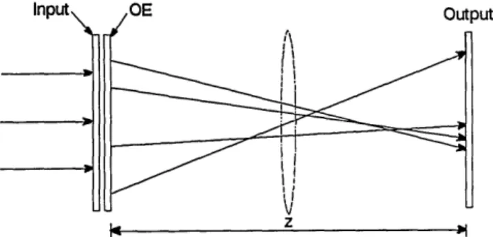
We review the main optical-coordinate transfor-mation methods, all of which are based on the arrangement presented in Fig. 1 or its equivalent. A two-dimensional input pattern is illuminated with collimated coherent light. A phase-modulating opti-cal element (OE) is placed in contact with the input mask. This OE can be a diffractive element (such as a hologram) or a refractive element. At the output plane we find the input pattern represented in the new coordinates. The distance between the input and the output planes is z. In some configurations a Fourier-transform lens is required (see Fig. 1). In these cases the focal length of the lens is f = z/2. We assume that the diameter of both the input and the output is D.

A. Bryngdahl's Method

The first method for performing coordinate transfor-mations was introduced by Bryngdahl (Fig. 1 with the dashed lens).9 His OE design is based on two approx-imations: the saddle-point approximation and the paraxial approximation (z >> D).3 The saddle-point approximation requires that we reduce z as much as possible, whereas the paraxial approximation re-quires that we increase z. This implies that this system could work well only with a large f-number (f#). From the geometric-shadow condition (which is fully equivalent to the saddle-point-integration condition), it can be shown3that the number of pixels

Input OE Output

z 1*

Fig. 1. General optical system for coordinate transformation. The dashed lens appears only in some of the mapping methods. In these cases, the focal length of the lens is f = z/2.

that this system can handle is

D

(1)

This value of N is much less than the space-bandwidth product of the optical system, given by

SW

where a diffraction-limited system has been assumed.

As explained above, f# >> 1 in Relations (1) and (2).

Another restriction of this method is that it is suitable only for certain types of transformation that can be derived from analytic functions. Unfortunate-ly, many coordinate transformations that are of interest in optical processing, for instance, the Carte-sian polar transformation, do not satisfy this condi-tion.

Because in most cases the OE function cannot be realized with direct optical (interferometric) methods, it is fabricated only with computer-generated holo-gram techniques such as computer-generated inter-ferograms.10 Thus in most cases performance is limited by the actual realization of the hologram. Another important parameter is the OE efficiency, which cannot be high with computer-generated holo-grams unless one is willing to use expensive OE manufacturing techniques. The first row of Table 1 summarizes the properties of Bryngdahl's method.

B. Multiple Holographic OE's

To generalize Bryngdahl's method to nonanalytic transformations, Stuff and Cederquist" recently sug-gested the use of a configuration with multiple OE's. The basic idea was to use the configuration of Fig. 1 (with the lens) twice in cascade. They showed that, subject to some requirements that can be met in most, perhaps all, practical cases, any one-to-one transformation can be performed with at most two OE's. Using this approach, they demonstrated the polar coordinate transformation.

Again the saddle-point and paraxial approxima-tions were made."1 As a result the performance of this system (which is shown in the second row of Table 1) is similar to that of Bryngdahl's method. The diffraction efficiency of the system is lower because it contains two diffractive elements in

cas-cade.

Table 1. Comparison of the Main Optical Coordinate Transformation Methods

Transformations

Method N(D) N(SW)a Possible Remarks

Bryngdahl D/Xf# TSWO Only analytic f# >> 1 Multiple OE's D/Xf# ASWL Almost every f# >> 1

k-vector =D/X \/W₂ Only analytic z D

Multifacet -D/X W2 Almost every z D

aSW₁, space-bandwidth product that is related to the f# >> 1

case; SW2, SW with f# 1 (z f D). Note that SW2 > SW,

because of the additional condition on the f#. 5120 APPLIED OPTICS / Vol. 32, No. 26 / 10 September 1993

C. k-Vector Method

Recently Davidson et al. 12suggested a new method for designing OE's for coordinate transformations that uses the optical setup of Fig. 1 without the dashed lens. The new method is based on analytic ray tracing and a geometric-shadow approximation that can be confirmed by the saddle-point approximation. The main advantage of this design is that the paraxial approximation is not necessary, so that the distance z between the input and output planes can be opti-mized to maximize N. It has been shown that the optical value of z is

Z= D,

(3)

which leads to

D

D

N = Dx -

D(4)

It can be seen that this value of N is greater than that given by Eq. (1), because f# >> 1. We are again restricted to analytic functions because the phase function of the OE is expected to be continuous.

D. Multifacet OE's

The most straightforward method of implementing optical map transformations is the multifacet ap-proach.'3 In this approach, an input light distribu-tion can be mapped to a fully arbitrarily prescribed output light distribution. The idea is to divide the OE into many small facets, one per input pixel. Each facet is a grating or microprism that diffracts or deflects the light toward the output pixel according to the transformation law. This method is similar to the k-vector method. Whereas the k-vector method is continuous, the multifacet approach is discrete. The multifacet approach has no restrictions about the transformation type, and every one-to-one trans-formation law can be achieved. In fact, this method can in principle also be extended to many-to-one or one-to-many transformation laws.

One of the main advantages of this technique is the high diffraction efficiency that it can provide when diffractive OE's are used. The recording of the holographic OE is done either by use of computer-generated holograms or by use of direct optical record-ing. In the second alternative, volume phase materi-als such as dichromated gelatin can be used to achieve nearly 100% diffraction efficiency. The number of pixels that the system can handle, N, is the same as that for the k-vector method as presented in the bottom row of Table 1.

E. Discussion

From Table 1 we conclude that there is no reason to use the continuous-phase methods (Bryngdahl, multi-ple OE's, and k vector). The multifacet approach combines flexibility and light efficiency with a value of N that is as good as the value obtained with the k-vector method and better than the values obtained

with the other methods, and thus it should be pre-ferred if we restrict ourselves to systems with at most one or two stages.

3. Optical-Interconnection Architectures

A large number of architectures for optical intercon-nection of electronic processing elements or optical switch arrays have been proposed. Those listed in Table 2 are representative of broad classes of essen-tially equivalent architectures. Methods similar to those occupying the first three rows of Table 1 are not considered, as they were found to be inferior in Sec. 2. We require that the architecture have the flexibility of being able to be customized such that any arbitrary pattern of one-to-one connections between N input and N output channels is possible. There are N! such patterns. (For readers familiar with Refs. 14 and 15, this corresponds to setting the parameter q = 1 in those papers. For other readers, we note that for special connection patterns exhibiting some form of locality or regularity, improvements over the values of Table 2 are possible.)

A. Matrix-Vector-Product Architectures

The first row of Table 2 is for optical-interconnection architectures based on so-called matrix-vector prod-ucts. These architectures are based on the well-known optical matrix-vector multiplier6 that is used to perform the operation

° = I Mjij

i

on a linear input array Ij of N elements to produce the result again in the form of a linear output array 0i of N elements. The N x N matrix by which the input is multiplied, Mij, is encoded as the transmittance func-tion of an N x N optical mask. To implement one-to-one interconnections, we simply set Mij = 1, if input i is to be connected to output j, and Mij = 0 otherwise. Thus any arbitrary interconnection pat-tern can be realized. For a one-to-one interconnec-tion pattern, only one element of the matrix will be nonzero in any row or column. If we assume lenses with an f-number f#, the distance from the input array to the mask must be at least zNf#X. The same distance is required from the mask to the output array; hence the linear longitude extent given in Table 2.

Table 2. Comparison of Optical Interconnection Architectures

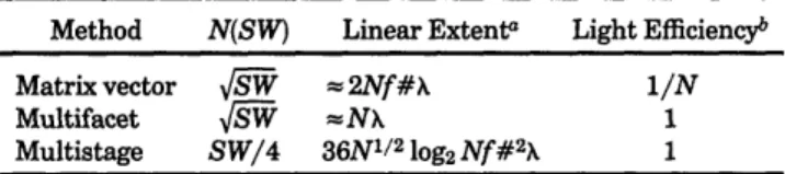
Method N(SW) Linear Extenta Light Efficiencyb

Matrix vector F/W = 2Nf#A 1/N

Multifacet SW = NX 1

Multistage SW/4 36N1/2log2Nf# 2

X 1 aThe linear axial extent of the system is important because it determines the propagation delay through the system. It is assumed that the source or detector sizes are not the limiting factor.

bFor an ideal system, ignoring coupling, radiation, attenuation losses, etc.

Because only N of the N2 mask elements are transparent, the light efficiency of this architecture is at best 1/N. This architecture has the potential to implement a full crossbar network with arbitrary fan-in and fan-out, but here we are interested only in one-to-one networks. It can also be dynamically reconfigured if a spatial light modulator with on-off transmittance is available.

B. Multifacet Architectures

The second row of Table 2 is for multifacet architec-tures (once again, we may refer to Fig. 1). Many essentially equivalent architectures have been sug-gested (for instance see Refs. 14 and 17-23). Here we assume that the number of facets is equal to the number of input and output channels. (In a system exhibiting some degree of space invariance, a smaller number of facets may be sufficient.'9) The light emanating from each source is directed toward the target detector with a dedicated facet element, which can be a hologram, a prism, etc. Thus any arbitrary pattern of interconnections can be implemented with equal ease. The number of input-output channels that one can have with these architectures is approxi-mately equal to (SW)1/2, as in the fourth row of Table 1. Because the axial extent of the optical system must at least be comparable with the diameter of the input plane D, the linear extent is given by NX [see Relation (4)]. We see that this architecture is prefer-able to the matrix-vector-product architecture be-cause the latter has poor light efficiency.

This architecture also allows a certain degree of

fan-out and fan-in by using multiple gratings.

Dynamic reconfiguration would require a variable-grating spatial light modulator or an array of active deflectors.

C. Multistage Architectures

The final line is for multistage architectures. It is well known that an arbitrary pattern of one-to-one interconnections can be realized in 3 log2N - 1 3

f

D

f 2f

f

log2 N stages, each involving a regular pattern of

interconnections followed by an array of local ex-change-bypass modules.19,2₄2 7 _{Because each stage}

involves a regular pattern of interconnections only, it can be implemented with near space-invariant optical imaging (i.e., the pupil plane is subdivided into only a small number of facets, say, 2 or 4).19 The space-bandwidth product needed is proportional to N, and the length of each stage is thus proportional to N'/2.

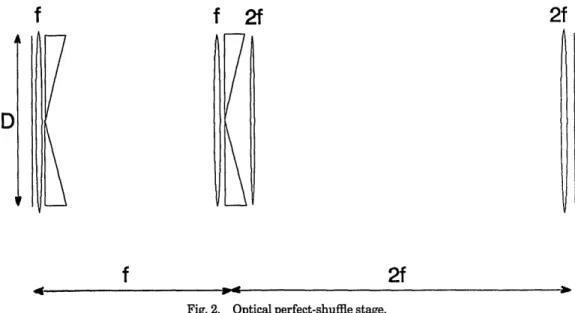
The perfect shuffle is a particular instance of the regular interconnections mentioned above. Figure 2 shows a single stage of a perfect-shuffle-based multi-stage system. It is a compact version of the one described in Ref. 25. The interface between consecu-tive stages could be accomplished with a telescope array device,2 8which can also perform the (passive) local exchange-bypass operations. The space-band-width product required is 4N because the pupil plane is divided into four parts. The length of each stage is

12Xf# 2N1/2

so that the length of the system is

36Xf# 2N1/2 log₂N.

(6)

(7)

This architecture is not as flexible as the matrix-vector architecture in terms of fan-in and fan-out, but it is nevertheless capable of realizing arbitrary one-to-one permutations. It can be dynamically reconfig-ured if the exchange-bypass modules are active switches, rather than passive couplers. This archi-tecture is asymptotically superior to the multifacet architecture. In fact the cost and the axial linear extent achievable with this system are only a logarith-mic factor worse than the fundamental limit given in

Ref. 14.

None of the above architectures imposes any restric-tions on the f#. If good quality lenses are used, it is possible to have f# 1.

Another architecture that is not included in Table 2

2f

2f

Fig. 2. Optical perfect-shuffle stage. 5122 APPLIED OPTICS / Vol. 32, No. 26 / 10 September 1993

is the three-dimensional multifacet architectures which approaches the fundamental limit within ap-proximately an order of magnitude, independent of N. Thus, for a large N, this architecture would be superior to those considered above. However, be-cause this architecture cannot be easily manufac-tured, it was not included in the above comparison.

4. Discussion and Conclusion

The multifacet and multistage architectures are flexi-ble techniques for implementing optical-coordinate transformations and optical interconnections. Fig-ure 3 illustrates the costs of the multifacet and multistage architectures as a function of N. The cost is defined as the cost of a single stage multiplied by the number of stages. We assume that the cost of a single stage is proportional to its SW. For the multifacet architecture that has only one stage the

cost is

CJSW = CN2, (8)

where C, is a constant with dimensions of cost. For the multistage architecture the cost of a single stage is

C2SW = CAN. (9)

In general we expect that C2 > C, because of the

more complicated optical configuration for the

multi-1017 1014 ._ 1n : M

c

stage architecture. The exact C, and C2parameters

depend on specification of the particular implementa-tion, and thus the ratio C2/C, is left as a parameter. In Fig. 2, three different ratios of C2/C, have been used: 1, 5, and 25. Simple interpolation could lead to the plot of other C2/C, ratios. It can be seen that until N 5000 (i.e., a two-dimensional array of

70 x 70 pixels), the multifacet architecture would be preferred because of its simplicity and lower cost. For high-performance optical computing and switch-ing systems with large N's, the multistage architec-ture is to be preferred.

It is often thought that there is a fundamental trade-off between efficient use of the space-band-width product and flexibility in implementing arbi-trary space-variant connection patterns. In particu-lar it is usually implied that SW oc N2 is needed to

realize an arbitrary permutation between N input

and output points. We have seen that for both optical-interconnection and transformation applica-tions, an SW of 4N is sufficient, which is only a factor of 4 worse than the fundamental limit. The price that was paid is that o log N stages were needed. Nevertheless, for a large N, the cost and linear extent of a multistage system will still be less than for the multifacet system.

Even the logarithmic factor is not a fundamental necessity, as the existence examples in Ref. 14 show. However, a practical system that requires an SW that

i04

N

Fig. 3. Cost versus number of pixels for the multifacet architecture (solid curve), and the multistage architecture (the dashed, dotted, and dashed-dotted curves correspond to C2/C, = 1, 5, and 25, respectively).

is not much greater than N and for which the linear extent is oc N1/2without the logarithmic factor has yet to be demonstrated.

This research was done while the authors were visiting the Applied Optics Group, Physics Institute, University of Erlangen-NUrnberg, Federal Republic of Germany. We thank Adolf W. Lohmann for sev-eral discussions and suggestions. David Mendlovic acknowledges receiving a MINERVA fellowship. Haldun M. Ozaktas acknowledges the support of the Alexander von Humboldt Foundation through a post-doctoral research fellowship.

References

1. J. Duvernoy, "Modele synthese non-lineaire pour le traitment optique des ecritures," Opt. Commun. 11, 373-377 (1974). 2. A. Sawchuk, "Space-variant image restoration by coordinate

transformation," J. Opt. Soc. Am. 64, 138-144 (1974). 3. D. Casasent and D. Psaltis, "Deformation invariant, space

variant optical pattern recognition," Prog. Opt. 16, 289-356 (1978).

4. Y. Saito, S. Komatsu, and H. Ohzu, "Scale and rotation invariant real time optical correlator using computer gener-ated hologram," Opt. Commun. 47, 8-11 (1983).

5. D. Casasent, S.-F. Xia, A. J. Lee, and J.-Z Shong, "Real-time deformation invariant optical pattern recognition using coordi-nate transformations," Appl. Opt. 26, 938-942 (1987). 6. D. Mendlovic, N. Konforti, and E. Marom, "Scale and

projec-tion invariant pattern recogniprojec-tion," Appl. Opt. 28, 4982-4986 (1989).

7. G. Hiusler and N. Streibl, "Optical compensation of geometri-cal distortion by deformable mirror," Opt. Commun. 42,

381-385 (1982).

8. A. W. Lohmann and N. Streibl, "Map transformations by optical anamorphic processing," Appl. Opt. 22, 780-783 (1983). 9. 0. Bryngdahl, "Geometrical transformation in optics," J. Opt.

Soc. Am. 64, 1092-1099 (1974).

10. W. H. Lee, "Binary synthetic holograms," Appl. Opt. 13, 1677-1682 (1974).

11. M. A. Stuff and J. N. Cederquist, "Coordinate transformations realizable with multiple holographic optical elements," J. Opt. Soc. Am. A 7, 977-981 (1990).

12. N. Davidson, A. A. Friesem, and E. Hasman, "Optical coordi-nate transformations," Appl. Opt. 31, 1067-1073 (1992). 13. S. K. Case, P. R. Haugen, and 0. J. Lberge, "Multifacet

holographic optical elements for wave front transformations," Appl. Opt. 20, 2670-2675 (1981).

14. H. M. Ozaktas, Y. Amitai, and J. W. Goodman, "Comparison of system size for some optical interconnection architectures and the folded multi-facet architecture," Opt. Commun. 82, 225-228 (1991).

15. H. M. Ozaktas, Y. Amitai, and J. W. Goodman, "A three dimensional optical inter-connection architecture with mini-mal growth rate of system size," Opt. Commun. 85, 1-4 (1991).

16. J. W. Goodman, A. R. Dias, and L. M. Woody, "Fully parallel, high-speed incoherent optical method for performing discrete Fourier transforms," Opt. Lett. 2, 1-3 (1978).

17. H. M. Ozaktas and J. W. Goodman, "Lower bound for the communication volume required for an optically intercon-nected array of points," J. Opt. Soc. Am., A 7, 2100-2106 (1990).

18. G. E. Lohman and A. W. Lohmann, "Optical interconnection network utilizing diffraction gratings," Opt. Eng. 27, 893-900 (1988).

19. G. E. Lohman and K.-H. Brenner, "Space-variance in optical computing systems," Optik 89, 123-124 (1992).

20. R. K. Kostuk, J. W. Goodman, and L. Hesselink, "Optical imaging applied to microelectronic chip-to-chip interconnec-tions," Appl. Opt. 24, 2851-2858 (1985).

21. R. Kostuk, J. W. Goodman, and L. Hesselink, "Design consid-erations for holographic optical interconnects," Appl. Opt. 26, 3947-3953 (1987).

22. M. R. Feldman, C. C. Guest, T. J. Drabik, and S. C. Esener, "Comparison between electrical and free space optical intercon-nects for fine grain processor arrays based on interconnect density capabilities," Appl. Opt. 28, 3820-3829 (1989). 23. M. R. Feldman and C. C. Guest, "Interconnect density

capabil-ities of computer generated holograms for optical interconnec-tion of very large scale integrated circuits," Appl. Opt. 28, 3134-3137 (1989).

24. A. W. Lohmann, "What classical optics can do for the digital optical computer," Appl. Opt. 25, 1543-1549 (1986). 25. A. W. Lohmann, W. Stork, and G. Stucke, "Optical perfect

shuffle," Appl. Opt. 25, 1530-1531 (1986).

26. K.-H. Brenner and A. Huang, "Optical implementations of the perfect shuffle interconnection," Appl. Opt. 27, 135-137 (1988). 27. M. J. Murdocca, A. Huang, J. Jahns, and N. Streibl, "Optical

design of programmable logic arrays," Appl. Opt. 27, 1651-1660(1988).

28. A. W. Lohmann and F. Sauer, "Holographic telescope array," Appl. Opt. 27, 3003-3007 (1988).