IEEE TRANSAmIONS ON PAmERN ANALYSIS AND MACHINE INTELLIGENCE, VOL. 16, NO. 8. AUGUST 1994 83 1
establish electrical connections between components on multilayered circuit boards. Conditions such as excess filling and lack of filling cause electrical defects. The sample shown in Fig. 9 has a cavity, indicating lack of filling. The specular reflectance and variable size of the tungsten particles gives the surface a random texture. In this case, a total of 18 images were taken using stage position increments of 8 gm. Some of these images are shown in Fig. 9(a)-(f). Fig. 9(g) and Fig. 9(h) show a reconstructed image and two views of the depth map, respectively. The image reconstruction algorithm simply uses the estimated depth to locate and patch together the best focused image areas in image sequence. The depths maps have been filtered using a 5 x 5 median filter to remove a few scattered erroneous depths that result from the lack of texture in some image areas.
VIII. DISCUSSION
The above experiments demonstrate the effectiveness of the shape from focus method. The results show that the Gaussian interpolation algorithm performs stably over a wide range of textures. No assump- tions are made regarding the type of the textures. Small errors in computed depth estimates result from factors such as. image noise, Gaussian approximation of the SML focus measure function, and weak textures in some image areas. Some detail of the surface roughness is lost due to the use of a finite size window to compute focus measures.
The above experiments were conducted on microscopic surfaces- that produce complex textured images. Such images are difficult, if not impossible, to analyze using recovery techniques such as shape from shading, photometric stereo, and structured light. These techniques work on surfaces with simple reflectance properties. Since the samples are microscopic in size, it is also difficult to use binocular stereo. Methods for recovering shape by texture analysis have been researched in the past. Typically, these methods recover shape information by analyzing the distortions in image texture due to surface orientation. The underlying assumption is that the surface texture has some regularity to it. Clearly, these approaches are not applicable to surfaces that produce random and spatially varying textures. For these reasons, shape from focus may be viewed as an effective method for objects with complex surface characteristics.
ACKNOWLEDGMENT
The authors would like to thank U. Shah for his help in implement- ing the automated system. This work has benefited from discussions with R. Willson of the VASC Group at CMU.
I11 121 131 [41 151 I61 171 181 REFERENCES
M. Born and E. Wolf, Princ.iples ofOptic,s. London: Pergamon, 1965. T. Darrell and K. Wohn. “Pyramid based depth from focus,” in Procc
CVPR. 1988. pp. 504-509.
J . Ens and P. Lawrence. “A matrix based method for determining depth from focus.” in Proc.. CVPR. 1991, pp. 606606.
P. Grossmann, “Depth from focus.” Portrrn Rwo,qiir. Lrrt.. vol. 5 . pp.
6 3 4 9 , 1987.
B. K . P. Hom, “Focusing.” MIT Aniticial Intell. Lab., Memo no. 160. May, 1968
-, Rohor Visio/i.
R. A. Jarvis, “Focus optimization criteria for computer image process- ing,” Mic~r.o.wopr. vol. 24. no. 2. pp. 163-180. 1976.
J. F. Koretz and G. H. Handelman. “How the human eye focuvs.” S c , i e t i r i f i c . American. pp. 92-99, July 1988.
Cambridge, MA: MIT Press. 1986.
191 E. Krotkov, “Focusing,” Inf. J . of Comput. Vision, vol. 1, pp. 223-237 1987.
[IO] G . Ligthart and F. Groen, “A comparison of different autofocus algo- rithms,” in Proc. of ICPR, 1982, pp. 597-600.
[ I I ] H. N. Nair and C. V. Stewart, “Robust focus ranging,” in Proc. CVPR, 1992, pp. 309-314.
[ 121 S. K. Nayar and Y. Nakagawa, “Shape from focus,” Tech. Rep., Dept. of Comput. Sci., Columbia Univ., CUCS 058-92, Nov. 1992. 131 A. Pentland, “A new sense for depth of field,” IEEE Trans. Pattern
Analysis and Machine Intell., vol. 9, no. 4, pp. 523-531, July 1987. 141 J. F. Schlag, A. C. Sanderson, C. P. Neumann, and F. C. Wimberly,
“Implementation of automatic focusing algorithms for a computer vision system with camera control,” Tech. Rep., Camegie Mellon Univ., CMU- 151 M. Subbarao, “Efficient depth recovery through inverse optics,’’ Machine Vision for Inspection and Measurement, H . Freeman, Ed.. New York: Academic Press, 1989.
161 M. Subbarao and G . Surya, “Depth from defocus: A spatial domain approach,” Tech. Rep. 92.12.03, SUNY, Stony Brook, Dec. 1992. [ 171 I. M. Tenenbaum, “Accommodation in computer vision,” Ph.D. thesis,
Stanford Univ., 1970.
[I81 R. G. Willson and S . A. Shafer, “Dynamic lens compensation for active color imaging and constant magnification focusing,” Tech. Rep., Camegie Mellon Univ., CMU-RI-TR-91, Oct. 1991.
RI-TR-83-14, Aug. 1983.
Gibbs Random Field Model Based Weight Selection
For The 2-D Adaptive Weighted Median Filter
Levent Onural, M. Bilge Alp, and Mehmet Izzet GurelliAbstract-A generalized filtering method based on the minimization of the energy of the Gibbs model is described. The well-known linear and median filters are all special cases of this method. It is shown that, with the selection of appropriate energy functions, the method can be successfully used to adapt the weights of the adaptive weighted median filter to preserve different textures within the image while eliminating the noise. The newly developed adaptive weighted median filter is based on a
3 x 3 square neighborhood structure. The weights of the pixels are adapted according to the clique energies within this neighborhood structure. The assigned energies to 2- or 3-pixel cliques are based on the local statistics within a larger estimation window. It is shown that the proposed filter performance is better compared to some well-known similar filters like the standard, separable, weighted and some adaptive weighted median filters.
Index Terms-Gihbs random field model, adaptive filtering, weighted median filter, image noise filtering.
I. INTRODUCTION
Median filters have the capability of preserving edge information in images while eliminating the noise components. This brings an advantage over linear filters which suffer from edge smoothing and blurring. Especially with impulsive noise (in general, if the noise distribution has long tails), median filters outperform their linear Manuscript received December 17. 1992; revised September 10, 1993. Recommended for acceptance by Associate Editor T. Caelli.
L. Onural and M. B. Alp are with the Department of Electrical and Electronics Engineering. Bilkent University, Bilkent. TR46533, Ankara, Turkey: e-mail: [email protected],
M. I. Gurelli is with the Signal Processing Institute, Department of Electrical Engineering-System,, University of Southem Califomia, Los Angeles, CA 90089 USA.
832 IEEE TRANSAmIONS ON PATTERN ANALYSIS AND MACHINE INTELLIGENCE, VOL. 16, NO. 8, AUGUST 1994
counterparts: they produce sharper images which are usually rated as “better” by observers. The interested reader is forwarded to the extensive literature on the subject (see for example, [l]).
In general, images contain parts with different characteristics. There can be homogeneous regions as well as regions with different textures within the same image. It is not possible for a single fixed filter to be effective in preserving all of these different characteristics. Therefore, to improve the performance in image filtering, adaptation of the filter parameters is desired. The first attempts toward achieving this goal with median-based filters are based on choosing the filter which gives the best possible output among several filters with different masks [2], [3], [4]. In [ 5 ] , shape and size of the median filter mask is adapted to the noise characteristics. However, the adaptation in all those approaches mentioned above is very limited. Other approaches use more general classes like rank order based filters [ 6 ] , or stack filters [7], and try to adapt the filter parameters in order to minimize a certain error criterion, such as mean square or mean absolute error, between the filter output and a reference training signal. Weighted median filters supply a simple and effective way for adaptation by adjusting the weights. This property has been used in [ K ] by changing the weight of the central pixel. In 191, adaptation is maintained by selecting among the several preset weighted median filters. However, in all these approaches the adaptation is limited because the choice of weights is restricted to be from a small set. To overcome this limitation, in [ 101 the weights are adjusted according to the local variance-to-mean ratio under the assumption that a high ratio indicates an edge whereas a low ratio is interpreted as a corrupted uniform region. Therefore, if the variance-to-mean ratio is low, the weights of the surrounding pixels are chosen to be closer to the weight of the central pixel to remove noise within the uniform region; otherwise, the central pixel weight is dominant and the edges pass rather undistorted. None of the adaptation methods mentioned above give satisfactory results when the input contains contaminated textural regions. In this correspondence, we propose a way to select the weights adaptively based on the local image statistics, with the aim of preserving different textures within the image. As a consequence of the proposed approach, not only the individual pixel values, but also pattems of groupings of these pixel values are effective in finding the output pixel. The proposed filter is not too complex for practical implementations, and it is suitable for cleaning corrupted images while preserving their texture.
It is also stressed, in this correspondence, that the median filter and its derivatives like the weighted median filter and the adaptive weighted median filter are all special cases of a more general class of filters. The linear filter is also a special case of the same class.
11. GENERALIZED FILTERING BASED ON THE GIBBS RANDOM FIELD MODEL
Let the input image be denoted as x and the output as y. The joint probability distribution of all input and output pixels is taken to be in the form of
P ( x. y ) = X*esp{ - C ( x. y ) } ( 1 )
which implies that the random field is a Gihhs random field (GRF). Details of GRF’s can be found in [ I l l and [12]. Here 1. is just a normalizing constant. The exponent I-(x.y), will be called the
energy of the input-output image pair under the specified model. It is known that the energy function associated with the input-output pair can be decomposed and written as the sum of clique potentials, as:
where c is the clique index; and the summation is over the set of all cliques. A clique is just an arbitrary subset of pixel sites. It is well known that the Gibbs random field and Markov random field models are equivalent under the positivity condition. However, the GRF approach is much simpler and does not need any explicit neighborhood and clique structure definitions [ I I]. Note that most of the clique potentials are zero. Therefore, one may represent the energy c’ as a sum over a much smaller set of cliques which may have nonzero potentials.
A general filter based on the GRF approach is an operator which maximizes the probability function with respect to y given a fixed input (observation) x:
But for a given input image
x,
P ( x ) is a constant, therefore, this maximization problem reduces to the minimization of the energy function:output = yo = iiiiii 17(x.y). (4)
Y
Each choice of the energy function,
I’,
yields another filtering operation. For example, the simple energy functionis associated with some well-known filtering operations. Choosing A - l ( y t ) = 0 and C(y,..r.,) = (y, - ~ , ~ . r . ~ ) ’ would result in a linear filtering operation. The standard median and weighted median filters can be obtained from this general form in a similar manner. Other selections of the A and C functions define other forms of filters which may be more useful for many applications.
Further generalizations are possible. The energy function
a11 , . I . pait-. nil k . I pa,,”
has a term ( D ) which models interactions among two input pixels and an output pixel, and another term ( E ) which models interactions among two output pixels. Thus it is possible to incorporate texture trends at the input while finding the output; and furthermore, some additional texture features can be imposed on the output. The linear and the commonly used versions of the median filter cannot detect and utilize texture trends at the input. “All i . j pairs,” under the summation signs mean that ( i . j ) is the same as ( j . i ) , so only one of them is included while summing. That statement also means that i
#
j must be satisfied while summing.Tww Special Cases - Linear and Median Filters: Let the energy function 17(x. y ) be given as:
where the indices i and j run over all pixels. In this case, the solution to the minimization becomes,
I
which is nothing but a linear filter. Here, it is assumed that both the input and the output data are S x -1- images. This filtering operation is equivalent to the optimal estimation problem where the observation x is the corrupted version of the original y with Gaussian noise,
r .
833 IEEE TRANSACTIONS ON PA'ITERN ANALYSIS AKD MACHINE INTELLIGENCE, VOL. 16. NO. 8. AUGUST 1994
such that ( y t - .rJ ) is a zero-mean Gaussian random variable for all ( i , j ) pairs with variance o:,. It is well known that the best (ML) estimate of yi given the observations is the linear combination of the observations. The weights of the linear filter al,'s are related to the variances ofJ 's.
Another example of the energy function is
In this case, the solution is
which is a weighted median filter [I31 whose definition is given in the next paragraph. The symbol
0
represents the weighting operation. This energy function and the associated median filter are analogous to the estimation of a value yt from its noise corrupted observations, .r, 's. Here the noise is biexponentially distributed around y, : in other words, .r, = yt+
n,,, and the distribution of the noise is [I41The weights n
,,
's are related to the distribution parameters a , 's. For integer weights, the weighted median filter is defined as follows: form a sequence of length a,, by repeating each sample.r, as many times as its weight a z J . Then sort the sequence and take the median value as the output. As the weight of a pixel increases, the likelihood of that pixel to appear at the output also increases. If all the weights are set equal to one, we get the standard median filter. By changing the weights, it is possible to change the root structure and the selectivity of the filter. Thus adaptive weighted median filter is obtained if the weights are adjusted according to the local properties of the incoming image. It is also possible to define the weighted median filter with noninteger positive weights. In this case, the weights should be interpreted as percentages: the ratio of the weight of a pixel to the sum of all weights is computed. These computed percentages are summed starting from the smallest pixel value going upward. The output is the value of the pixel which crosses the 50% barrier. If there are some negative weights, a constant should be added to all weights so that they all become positive.
The discussion presented in this section helps designers to find out novel filter structures and predict their performances under different circumstances. In this correspondence, a novel adaptive weighted median filter structure will be proposed based on this kind of approach.
111. ADARIVE WEIGHTED MEDIAN FILTER BASED ON THE GRF MODEL
Suppose that the energy term associated with the GRF model is chosen to be in the form of
Similar to the case given by (9) and (lo), the solution to this minimization is the weighted median filter:
Let us define a neighborhood, i l l , associated with each output site i . For simplicity, the elements of are chosen among the input pixels, only. The
G
functions are chosen to have(14)
G I , ( . ~ , )
= 0. if .r, I ) , .Furthermore, suppose that it is guaranteed to have Gl,(.r,)
+
Gzl ( .r,. x k )
2
0. Thus the problems associated with negative weights are eliminated. In this case, the output pixel will be:The weights of the above filter are the functions of the input pixel locations and values. The weight for pixel s, has two components. The first component adjusts the weight according to the value and the position of the associated pixel s,
.
The second component makes further adjustments based on pairs of pixels: each pair is formed by the pixel sJ and another pixel X k within the window. All such pairsformed by changing .rk are effective in finding the weight for T,. Of course, now the crucial point is the proper selection of the
G
functions. Some practical examples are given below. Conditions of equation (14) are all enforced in the examples, so they are not written explicitly again.Example I: The first example which yields an adaptive smoothing operator is,
Note that the
G
functions are already chosen to have 0 values outside the neighborhood as explained in the previous paragraph.T
is just a threshold value. To see the effect of the above selection, suppose that the neighborhood qz is the simple 3 x 3 window. The total weight of an element will not depend only on its location within the window (as in the conventional weighted median filter) but also on the values of other pixels in the window. If there is no pixel, among the eight other pixels, whose value comes close to the value of a pixel, its weight will be k. If there is only one pixel, among the other pixels, whose value is close to the value of the pixel, then the weight will be k+
1. The more similar values in a window, the more the weight of that pixel will be. Thus, this filtering operation will enhance the similarities (a strong smoothing operator) among the pixels when generating an output.Example 2: Another slightly more complex example may take into account the directional properties of the grouping tendencies. Consider the simple 3 x 3 window with the pixels indexed as shown in Fig. 1. Different weights may be assigned to horizontal, vertical or diagonal groupings as:
Here, if the central pixel takes a value close to one of its neighbors, then its weight is adjusted. The relative values of I , , h , n? or r determine the tendency at the output toward more vertical, horizontal, main-diagonal and reverse-diagonal stripes, respectively. The sensi- tivity to additional weights are adjusted by the relative values of a ,t 's.
Note that the output y, can be computed if all the input values within the window are known. Larger windows are always possible to model more complex direct interactions, but this will result in more
834 IEEE TRANSACTIONS ON PATTERN ANALYSIS AND MACHINE INTELLIGENCE, VOL. 16, NO. 8, AUGUST 1994
Fig. 1. Indexing in the 3 x 3 square window.
complicated filter structures. However, it is possible to bring longer interactions into the picture as shown by the following example.
Example 3: The goal is to detect the textural tendency of a local region using a rather uncomplicated method, and then to adapt the median filter weights to eliminate the noise which disrupts the detected texture. The filter size in this example is 3 x 3, but the region where statistics are gathered is larger. Suppose that there are
li pixels in region
R.
Let us defineU = median{lr, - m ( ( i E R ) and similarly, m, = m e d i a n ( ( r , - .r,,(Iz E
R}
U, = median (19) Is1 - sZ,( - m,( 1 ER
.
(I
I
}
Here m gives the mid-value of the pixels in the region, and, ~7 gives
the mid-value of the deviation from the mid-value [15]. Similarly, the m , is the mid-value of the difference of the pixel located at relative position n compared to the central pixel. orL is a measure of the deviation of the differences. If desired, more conventional mean and standard deviation can be used, but this may result in poor filter performance when the contaminating noise is impulsive. To reduce the complexity, an approximate median, which is obtained by coarse quantization of the input values and using a histogram to find the median of these quantized values, is sufficient. Once these statistics are measured within R, the G I , and G2, functions can be chosen. The adaptation of the central pixel will be considered first. G I , is defined as follows:
G l t ( . r t n ) = c , n = 2;..,9 (20)
where c and cen are constants. Here the rationale is to increase the weight of the central pixel if it already matches the statistics; otherwise, its weight is decreased. The results of different choices for these constants will be discussed after the adaptation due to other effects is also given. The additional adaptive weight due to G2, for the central pixel (i.e. for j = 8 ) is defined as follows:
G z r ( x , , s , , ) =
{
;"
e
e ( m r , - ( s t - .rnnIJ>
Ttlrgk,.ulr (21)othewise.
Here, uave is the mean of u T t , n = 2..
. .
,9, andZuw
andZ , r g ~ l
are two parameters given to adjust the selectivity of the filter. The above definition is illustrated in Fig. 2. The interpretation is as follows: if the central pixel fits the estimated statistics, it is less likely to be corrupted by noise. So its weight is increased in order to preserve the value of the input pixel. If the central pixel strongly violates the statistics of the region, then it is highly likely to be corrupted by noise. So its weight is decreased. However, in between, i.e., if the mismatch is not strong enough, we cannot arrive at a positive or negative conclusion,E
lm,, - Is, - S t J<
Tl<,w.~,tso we do nothing. If c is significantly large compared to the other additional weights, then the filter behaves more like the standard median filter. Higher values of cen will shift the behavior of the filter toward a center weighted filter, and the adaptation will be based more on the single pixel distribution statistics. Couplings of pixel pairs also affect the center pixel weight as adjusted by
z,,,
andTI,^^,,.
If Tic,wand T h i g h are high, the weight of the central pixel will probably be
increased and the output yt will probably take the value of the input. In this case, the texture in the image will be preserved. However, noise attenuation will be low. If the thresholds are small, the weight of the central pixel will probably be decreased and the probability of the output taking the value of the neighboring pixels will increase, thus the filter will act as a correction filter.
If the central pixel is corrupted. as understood from the mismatch of the central value to the statistics, then it must be replaced by one of the neighborhood pixels. Which neighborhood pixel will replace the central pixel is also determined from the weights of the noncentral pixels that are adjusted according to the statistics, as follows:
G z l ( . r J , z k ) = 0, f o r k
# i .
(22)U, nz,,
I
T , G Z ~ ( X ~ , ~ , Z ~ ) = a, n~,,>
2T,otherwise.
{
;-":
The adaptive weight assignment rule is illustrated in Fig. 3. This selection of noncentral weights can be interpreted as follows: if the estimated value of the difference Is, - .r,,,I, using (19), is small compared to a given threshold T, i.e., if x,,, tends to be similar to s,, then there is a strong positive coupling between .r, and .rt,,. So increase the weight of .rzn and thus increase the likelihood of the output y, to take a value close to the value of sL,, to form a pair. If the estimated difference tends to be large, then it is understood that there is a strong repulsion between s, and x,,. In this case, decrease the weight of .rt, and thus decrease the likelihood of the output y, to take a value close to the value of s,,,
.
If the estimated difference is neither small nor large, then there is no significant coupling between x 2 and x,,, so do not change the weight of x , , , . The steps to increase or decrease the weights depend on the estimated deviations which is given by (19). If the estimated deviation is small, the step size is large, because the coupling tends to be more consistent. The threshold parameter T determines when the couplings (either similarity or repulsion) will start affecting the weights: if T is larger (smaller), then the same statistics will be more likely to be interpreted as a positive (negative) coupling.It is possible to choose R in many ways. The optimum results would be obtained by the segmentation of the image into regions with different textures, and by considering each region as the R for the output pixel locations within that region. However, the segmentation process increases the complexity of the filter. So, in practice it is easier to partition the image into fixed regions. For example, the image may be partitioned into blocks and each block may be the
R
for the output pixel locations within that block. This will result in well-known blocking effect. Another choice is a constant shape which slides with the output pixel location i , i.e., another larger window. In any case, the size selection is another issue.
Iv. SIMULATIONS AND RESULTS
To evaluate the performance of the weight adaptation algorithm based on the GRF model, the filter given in Example 3 of Section 111 is implemented. The estimation of the image statistics is carried out on 8 x 8 nonoverlapping square blocks using the approximate median computation described in the previous section. Subjective evaluation and mean-square error (mse) are used as the error criteria. The performance of the GRF-based adaptive weighted median filter
IEEE TRANSACTIONS ON PATTERN ANALYSIS AND MACHINE INTELLIGENCE, VOL. 16, NO. 8, AUGUST 1994 835 ADDITIONAL o,,,
. -
WEIGHT
1+
on
I I I I I 1 I I I I I I I I I 0 l o , , , I;
l + o n;
I I I I 0 I --
Gave;
I + % I I I I I I I I I I I I I I I I I I I I I I I I I;
mn I I I I I I I I I I I 1 ( - - - I7
II
2Tlow 0, I I7
I 2Thighon e-- - -
- - - -
I I I I IFig. 2. The additional adaptive weight assignment to the central pixel due to Gzz. (The given function, which represents the density of the distribution of l x , - x t n
1,
is arbitrary.) mn ADDITIONAL WGtU 4 V C ’ t o , ~ 0 - 4VL ‘ + 4Fig. 3. The adaptive weight assignment rule for the noncenter pixels. (The functions, which represent the density of the distribution of I.r, -
1,
are arbitrary.)developed in this correspondence is compared with the standard median filter, the separable median filter [16], a center weighted median filter, and an adaptive weighted median filter [lo]. The window size is 3 x 3 for all filters. The separable filter operates horizontally at its first pass. The center weighted median filter has fixed center weight which is equal to five; all other eight pixels have unit weights. The image “BABOON” is used in the simulations. It has
TABLE I
MSE BETWEEN THE ORIGINAL TEST IMAGE AND THE FILTER
G
RF-based
3-point
median
median
median
14.013
21.655
21.698
OUTPUTS FOR IMPULSIVE NOISE WITH PROBABILITY 0.1
adaptive weighted
standard
separable
Adaptive weighted
~~median
1
w = 5 , c = l , K = l
I
17.288
I
22.044
The parameters for the GRF-based adaptive weighted median filter are:
c = cen = 1, T = 40, Tlow = 1.5 and Thigh = 3.0.
both homogeneous and highly textured regions. The original image is contaminated by an impulsive noise of probability 0.1 with equally likely positive and negative impulses. Although the performances of the filters are almost equal in homogeneous areas, the GRF-based adaptive weighted median filter outperforms the others in highly textured regions. This can be observed in Fig. 4 where the first quarter of the image is shown. The mse of the filter outputs are given in Table I. As can be observed from the calculations the adaptive weighted median filter improves the mse significantly.
The filter proposed in [lo] is developed with exactly opposite motivations: it is assumed that the object embedded in an ultrasound image is smooth whereas the corrupting noise is colored (speckle noise), and thus, have specific textural tendencies. So, the goal is not to pass the texture, but to eliminate it. Therefore, the filter performance is poor if the original is textured. Our observations based on the implementation of that filter confirms the poor performance of the filter when cleaning the corrupted “BABOON’ image shown in this correspondence.
836 IEEE TRANSACTIONS ON PATTERN ANALYSIS AND MACHINE INTELLIGENCE, VOL. 16. NO. 8, AUGUST 1994
Fig. 4. First quarter of the original “BABOON’ sequence and the filter outputs for impulsive noise with probability 0.1. (a) Original image. (b) Corrupted image. (c) GRF-based adaptive weighted median filter with TI,,, = 1.5 and Ttllgh = 3.0. (d) The standard median filter in a 3 x 3 window. (e) The 3-point separable median filter. (f) The center weighted median filter in a 3 x 3 window.
(a) (b)
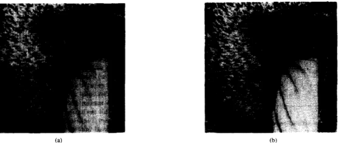
Fig. 5. The GRF-based adaptive weighted median filter outputs for impulsive noise with probability 0.1 for various threshold levels. (a)
T,,,,
= 0.25and
ThrKk,
= 0.75. (b)q,,,
= -1.0 and Ttlirl, = 6.0.Finally, the effect of the threshold levels,
T,,,,
and Tt,rgtrr on the performance of the GRF based adaptive weighted median filter can be observed in Fig. 5 and Table 11: if the threshold levels are high, the filter has a higher tendency to preserve the input, and this results in a poor noise elimination performance. If the threshold levels aretoo low, the filter loses its advantage in the textured areas and its performance gets closer to the standard median filter. However, it is possible to tune the thresholds so that a high noise attenuation is obtained while keeping the details of the image, as the mse figures in Table I1 show.
IEEE TRANSACTIONS ON PATTERN ANALYSIS AND MACHINE INTELLIGENCE, VOL. 16, NO. 8, AUGUST 1994 837
TABLE I1
MSE BETWEEN THE ORIGINAL TEST IMAGE A N D THE GRF-BASED ADAPTIVE WEIGHTED MEDIAN FILTER FOR VARIOUS THRESHOLD LEVELS
I
&,,,
= 0.25
I
=
1.5
I
= 4.0
I
Thigh
=
0.75
I
Thigh = 3.0I
T h i g h= 6.0
20.615
I
14.013
I
15.086
The parameters for the GRF-based adaptive weighted median filter are:
f = C P 7 t = 1 . T = 40.
V. CONCLUSION
There are various edge preserving smoothing nonlinear filters in the literature. Among these the median filter and the weighted median filter have gained a good reputation. However, these filters do not show acceptable performances when the filtered regions are textured. The adaptation algorithm presented in [IO] uses variance-to-mean
ratio to adapt the filter weights. This feature is not suitable for cleaning impulsive noise corrupted textured images, and therefore, the filter performance is poor in such environments. The presented GRF based adaptive weighted median filter is capable of tracking the local texture behavior while cleaning noise as a result of the weight selection algorithm which is based on the local statistics of pixel couplings. The improvement in the performance is significant especially in textured images, as expected. Even though the filter complexity is higher than the above mentioned filters, it is still acceptable for many practical applications.
The presented GRF based filter design approach is a general method which is not limited to median filters. Various other adaptive filters may be developed using similar local statistics within different filter structures which minimize different energy functions.
REFERENCES
0. Yli-Harja, J. Astola, and Y. Neuvo. “Analysis of the properties of median and weighted median filters using threshold logic and stack filter representation,” IEEE Trans. Signal Processing. vol. 39. no. 2. pp. 395410, Feb. 1991.
P. Heinonen, and Y. Neuvo, “FIR-median hybrid filters,’’ IEEE Truns.
Acoust.. Speech. Signal Proc,essing. vol. ASSP-35, pp. 832-838, June 1987.
G. R. Arce and M. P. McLoughlin, “Theoretical analysis of the max/median filter,” IEEE Trans. Acousr.. Spewh. Signol Processing.
vol. ASSP-35, pp. 6 0 4 9 , Jan. 1987.
S.-J. KO, Y. H. Lee, and A. T. Fam, “Selective median filters.” in
ISCAS’RR, 1988, pp. 1495-1498.
H.-M. Lin and A. N. Willson, “Median filters with adaptive lengrh,” IEEE Trans. Circuits Syst.. vol. 35, no. 6, pp. 675-690, June 1988.
P. Salembier, “Adaptive rank order based filters,” Signal Prrxessing. vol. 27. pp. 1-25, 1992.
L. Yin, J. T. Astola, and Y. A. Neuvo, “Adaptive stack filtering with application to image processing,” IEEE Trans. Signal Proc,essing. vol.
41, no. 1, pp. 162-184, Jan. 1993.
R. Kutka, “A variable median filter for image restoration adaptable to different types of spike noise,” Signal Processing. vol. 18. no. 2, pp.
217-224, Oct. 1989.
S. S. Perlman, S. Eisenhandler, P. W. Lyons, and M . J. Shumila, “Adaptive median filtering for impulse noise elimination in real-time TV signals,” IEEE Trans. Commun.. vol. COM-35, no. 6. pp. 646-652. June 1987.
T. Loupas, W. N. Mcdicken, and P. L. Allan, “An adaptive weighted median filter for speckle suppression in medical ultrasonic images,” IEEE Trans. Circuits Syst.. vol. 36, no. I. pp. 129-135, Jan. 1989. H. Derin and H. Elliot, “Modeling and segmentation of noisy and textured images using Gibbs random fields,” IEEE Trans. Pattern Anal.
Machine Intell.. vol. PAMI-9, no. I , pp. 39-55. Jan. 1987.
[ 12) S. Geman and D. Geman, “Stochastic relaxation, Gibbs distributions, and the Bayesian restoration of images,” IEEE Trans. Pattern Anal.
Machine Intell., vol. PAMI-6, no. 6, pp. 721-741, Nov. 1984.
[ 131 D. R. K. Brownrigg, “The weighted median filter,” Commun. ACM, vol.
27, pp. 807-818, Aug. 1984.
[ 141 J. Astola, P. Haavisto, and Y. Neuvo, “Vector Median Filters,’’ in Proc.
IEEE, vol. 78, no. 4, pp. 678689, Apr. 1990.
[ I S ] M. I. Gurelli and L. Onural, “The adaptive directional median filter,” in
Proc. Sixth Int. Symp. Comput. Inform. Sci., Side, Turkey, vol. 11, Oct.
1991, pp. 973-979.
1161 T. A. Nodes and N. C. Gallagher, “Two-dimensional root structures and convergence properties of the separable median filter,” IEEE Trans.
Acoust.. Speech. and Signal Processing. vol. ASSP-31, no. 6 , pp. 1350-1365, Dec. 1983.
On the Discriminatory Power of Adaptive
Feed-Forward Layered Networks
Hossam Osman and Moustafa M. FahmyAbstract-This correspondence expands the available theoretical frame- work that establishes a link between discriminant analysis and adaptive feed-forward layered linear-output networks used as mean-square classi- fiers. This has the advantages of providing more theoretical justification for the use of these nets in pattern classification and gaining a better insight into their behavior and about their use. We prove that, under reasonable assumptions, minimizing the mean-square error at the net- work output is equivalent to minimizing the following: 1) the difference between the optimum value of a familiar discriminant criterion and the value of this criterion evaluated in the space spanned by the outputs of the final hidden layer, and 2) the difference between the values of the same discriminant criterion evaluated in desired-output and actual-output subspaces. We also illustrate, under specific constraints, how to solve the following problem: given a feature extraction criterion, how the target coding scheme can be selected such that this criterion is maximized at the output of the network final hidden layer. Other properties for these networks are explored.
mean-square optimization, discriminant analysis, Bayes risk.
Index Terms-Adaptive layered networks, pattern classification, least-
I. INTRODUCTION
As mean-square classifiers, adaptive feed-forward layered networks have shown a good performance in quite a significant variety of problems [ I]-[4].
Establishing a link between these networks and discriminant anal- ysis is of significant importance, since it provides more theoretical justification for the use of these nets in pattem classification, and it yields more insight into their behavior and about their use. Recent work has addressed the problem of establishing such a link, and has indicated that the high ability of these networks to perform pattem classification is mainly due to the discriminatory power of their hidden layers. For instance, Gallinari et al. [5] have shown that, under certain reasonable assumptions, a 3-layer linear network maximizes, at the output of its hidden layer, a discriminant criterion involving the ratio of the determinants of the between-class and Manuscript received October 5 , 1992; revised April 22, 1993. This work
was supported by the Canadian Natural Science and Engineering Research Council (NSERC) under Research Grant A4149. Recommended for accep- tance by Associate Editor R. W. P. Duin.
The authors are with the Department of Electrical and Computer En- gineering, Queen’s University, Kingston, ON, K7L 3N6, Canada; e-mail: [email protected].
IEEE Log Number 9403153.