*The authors would like to acknowledge the helpful comments and constructive criticisms of the editor and the three anonymous referees. Special thanks go to Sidika Basci who carried out the simulations. The authors are also indebted to the useful discussions and suggestions of seminar participants at Warwick Business School, CEFES Meeting at Cambridge University, METU Conference on Economics, European Financial Management Association and EURO Working Group on Financial Modeling.
(Multinational Finance Journal, 1999, vol. 3, no. 4, pp. 223–252)
©Multinational Finance Society, a nonprofit corporation. All rights reserved.
Financial Crisis and Changes in Determinants
of Risk and Return: An Empirical Investigation
of an Emerging Market (ISE)*
Gulnur MuradogluUniversity of Manchester, U.K. Hakan Berument Bilkent University, Turkey
Kivilcim Metin Bilkent University, Turkey
This paper examines how determinants of volatility and stock returns change with financial crisis. The contributions of the paper are twofold. First, using a GARCH-M framework, risk and return are jointly modeled by using macroeconomic variables both in the variance and the mean equations. The conditional variance equation is specified by including macro-economic variables, a relevant information set for emerging economies, that is often overlooked in various GARCH specifications. Second, determinants of risk and return are investigated before during and after a major financial crisis at ISE. We show that, both the determinants of risk and the risk-return relationship change as the economy switches from one regime to the other (JEL: G1,G2,C5).
Keywords: emerging markets, financial crisis, GARCH-M, Istanbul Stock
Exchange, macroeconomic variables, risk, stock returns
I. Introduction
Engle (1993, p. 72) states that "…financial market volatility is predictable, [and] this observation has important policy implications for
asset pricing and portfolio management." Clearly, assuming that investors generally are risk-averse, asset prices should respond to forecasts of volatility. Predicting risk, however, remains difficult since economists disagree on the major sources of risk. The Capital Asset Pricing Model (CAPM) of Sharpe (1964) and Lintner (1965) use the market return, and traditional Arbitrage Pricing Theory (APT) models such as Ross (1976) gives way to employ any other variables as the theoretical source of risk. Macroeconomic variables constitute an important set of information in several specifications of APT models. Macro-economic fluctuations are modeled assuming that they influence stock prices through their effect on future cash flows and rates used in discounting them.
In these models, volatility and related risk premiums are expressed in terms of asset covariances with the implied source of risk. The fact that assets with high expected risk must offer higher rates of return indicates that increases in the conditional variance should be associated with increases in the conditional mean. In this context, the Generalized Autoregressive Conditional Heteroscedastic in Means (GARCH-M) model provides a convenient instrument to incorporate time-varying risk premia as the specification of the mean in the stock return equation. GARCH-M is a time series process, which explicitly incorporates the risk-return relationship and the time-varying risk premium. Changes in determinants of risk, and the risk-return relationship are important in deciding on the appropriate cost of capital in international asset allocation.
In this paper, we examine the determinants of risk as well as the relationship between risk and return by using different specifications of GARCH-M models as the economy progresses through diverse stages. In this work we use macro-economic variables in the conditional variance equation. Previous studies have used various variables in modeling asset returns, but macro-economic variables have not been used to model conditional volatilities in an emerging market setting. Analysis of changes in the determinants of volatility and asset returns at various stages of a financial crisis in an emerging economy gives insights about a better understanding of the worldwide crisis triggered by crisis in emerging economies.
II. Review of Literature
The level of real economic activity is expected to have a positive effect on future cash flows and thus affect stock prices in the direction cash
flows are affected. Studies investigating the effect of macro-economic variables mainly employ conventional time-series models in their analysis. Arbitrage Pricing Theory (Ross, 1976) does not specify the individual economic variables as risk factors and leaves this issue to empirical researchers. Empirical work provides evidence for a number of macro-economic variables some of which we discuss below.
Geske and Roll (1983) argue that exchange rates influence stock prices through the terms of trade effect. Depreciation of domestic currency is expected to increase volume of exports. As long as demand for exports is elastic, this, in turn, will increase cash flows of domestic companies and thus stock prices. Share prices of companies with a higher foreign exchange rate exposure react more strongly to devaluation than those with lower levels of exposure (Pettinen, 2000). Malliaropulos (1998) supports these results by presenting a pronounced effect in relative performance of international equity portfolios. In countries where the currency appreciates in real terms against the dollar, the stock markets outperform the US stock market. Ajayi and Mougoue (1996) on the other hand, report international evidence about the feedback relation between stock markets and foreign exchange rates and show that currency depreciation has negative effects on the stock market both in the long run and the short run. They argue that inflationary effects of domestic currency depreciation may exert a moderating influence in the short run and unfavorable effects on imports and asset prices will induce bearish trends in the long run.
Although the relationship between inflation and stock prices is highly controversial, empirical studies mainly document a negative relation (Fama and Schwert, 1977). An increase in inflation is expected to increase nominal discount rates. If contracts are nominal and cash flows cannot increase immediately, the effect of a higher rate used to discount cash flows will be negative on stock prices. If high frequency data such as daily data is used it is not possible to use actual inflation rates. In this case several measures of money supply can be used as proxies. Note here that the effect of increases in nominal interest rates will be negative on stock returns in this argument.
While conventional time series models operate under the assumption of constant variance, the GARCH-M process allows the conditional variance to change over time as a function of past errors and of the lagged values of the conditional variance; still the unconditional variance
1. See Bollerslev, Chou and Kroner (1992) for a detailed review of literature.
remains constant (Bollersev, 1986). Measuring conditional variance has been found to be useful in modeling several economic phenomena such as inflation, interest rates (Engle, Lilien and Robins, 1987), and foreign exchange markets (Kendall and McDonald, 1989). In more recent studies researchers have found GARCH (1,1)-M an appropriate model for financial data as well.1 For example, using a GARCH(1,1)-M
formulation in the implementation of a CAPM model for a market portfolio consisting of stocks, bonds and bills, Bollerlsev, Engle and Wooldridge (1988) report a significant trade-off among these asset categories. Furthermore, in a univariate framework, Glosten, Jagannathan and Runkle (1993) show that the sign of the Autoregressive Conditional Heteroscedastic in Means (ARCH-M) model’s coefficients are sensitive to the instruments which are added to the mean and variance equations of the model. Attanasio and Wadhwani (1989) find that predictability of stock returns can be explained by a risk measure using ARCH, while other explanatory variables such as lagged nominal interest rates and inflation rates remain significant in explaining the movement of expected returns in addition to their own conditional variance.
GARCH-M modeling has been used, with mixed results, in several US and UK studies to examine the relationship between risk and return. French, Schwert and Stambaugh (1987) found evidence that expected market risk premium is positively related to the predictable volatility of stock returns in the US market, while Baillie and De Gennaro (1990), who studied similar data, found this relation weak. In the UK market, Poon and Taylor (1992) also reported that estimates of risk using the relevant GARCH-M parameter are not statistically significant.
Because of these mixed results, the literature contains extensive analysis of the empirical relationship between risk and return in mature markets, with scholars generally preferring one of two competing hypotheses to explain market behavior. After the 1987 crash, some researchers hypothesized a negative relation between unexpected returns and unexpected volatility, based on the assumption that when returns are lower than average, speculative activity is induced and market volatility increases (Poon and Taylor, 1992). The competing hypothesis suggests a positive relationship between expected returns and
2. See for example Errunza et al., 1994; Harvey, 1995; and Bekaert and Harvey, 1997.
3. See Im and Kim (1998) for an overview of the conditions that led to the 1997 financial crisis South Korea.
expected volatility, assuming that equity risk premiums provide compensation for risk when volatility increases.
Modeling risk and empirical tests of the relationship between risk and return are particularly important in emerging markets2 where volatility
is inherently high and changing over time. Cross-sectional models show that lower volatilities are observed in more open economies and countries that went through capital market liberalization (Bekaert and Harvey, 1997). However, in studies of the forces that determine volatility, macroeconomic variables, an important information set for the emerging markets of the developing economies, are not given due attention.
Especially, following the 1998 Asian Financial Crisis, the need arises to understand the emerging markets better. Kaminsky and Reinhart (2000) rigorously show that the crisis in emerging markets can be spread into the rest of the world, through trade and financial sector links as we are moving towards a more global economy. Still, the conditions that may lead to a crisis in an emerging economy can be unique to that economy and naturally different from those in developed countries. In most cases, emerging markets are not informationally efficient, and speculative activity is common due to thin trading (Muradoglu, 2000) and informational asymmetries (Balaban and Kunter, 1997). Also, the thinly traded stock markets of these controlled economies may go through crisis periods induced by fiscal and monetary changes. Since, in these markets, volume of trade is relatively low and publicly available information on company performances is limited, stock returns are also relatively more sensitive to economic policy actions (Muradoglu and Metin, 1996; Balaban, Candemir and Kunter, 1997).
To help fill in the gap in the finance literature about crisis in emerging economies, this paper investigates a financial crisis in an emerging economy. In many respects the 1994 financial crisis in Turkey developed similar to the 1997 crisis in Korea,3 but the consequences were not
global. The definition of financial crisis always includes increases in risks and changes in risk-return relationships. The question of whether
volatility and the economic factors that might affect volatility differ during changing economic conditions is an important issue. Changes in determinants of risk as well as the relationship between risk and return are important in determining the appropriate cost of capital and in evaluating foreign direct investments in emerging economies as well as international asset allocation decisions.
In this paper, we examine the determinants of risk as well as the relationship between risk and return before, during and after a major financial crisis in 1994 at the Istanbul Stock Exchange (ISE). Different specifications of GARCH-M models are employed. Results show that (1) risk, (2) asset returns and (3) risk-return relationships are affected by macroeconomic outcomes differently as the economy progresses through diverse stages.
The contributions of this study are twofold. First, to our knowledge, this is a leading work that uses macro-economic variables in the conditional variance equation. Asset returns and related conditional volatilities are modeled using a GARCH-M framework. Previous studies have used various variables in modeling asset returns, but macro-economic variables have not been used to model conditional volatilities in an emerging market setting. Second, investigation of changes in the determinants of volatility and asset returns due to a financial crisis in an emerging economy will give valuable insights to those who would like to understand the 1998 world crisis better.
Our study employed the following procedure. We first verified the before-during-after crisis periods by determining the possible changes in the estimated coefficients of a time series representation of the stock market. Next, we determined the order of the autoregressive process for each sub-period. Then we modeled risk by using the conditional variance specification and tested for the effect of risk on stock returns during each sub-period. In this process, we examined the possible macroeconomic determinants of risk in the stock market as well as testing for their conceivable effects on stock returns.
Accordingly the paper is organized as follows. After presenting a brief description of the Turkish stock market in Section 3, we outline the definitions and time series properties of the data in Section 4. Section 5 presents the methodology used and is followed by sections 6 and 7, the analysis of empirical results and related discussions. Finally, Section 8 provides conclusions.
III. The Turkish Stock Market
With the implementation of an IMF-supported stabilization program in 1980, the Turkish economy switched from an inward-looking development strategy to an outward-oriented one. The major components of the program included financial liberalization and the integration of financial markets. As an immediate result, in 1986 the Istanbul Securities Exchange (ISE) opened with 42 listed companies. In 1989, the Turkish financial system was further liberalized and foreign investors were permitted to hold stock portfolios at ISE. Since November 1994 all stocks, which totaled more than 250 by 1997, have been traded by a computer-assisted system. Daily trading volume has exceeded $150 million. In trading volume, ISE has become the eighth largest of the twenty-two European stock exchanges, surpassing Madrid, Copenhagen, Oslo, Brussels and Vienna. Similar to other emerging markets, ISE’s return volatilities have been high throughout its history. The ISE composite index measured in US dollars has increased by six-hundred percent since its establishment. This increase has been realized including annual increases up to 350%, followed by corrections amounting to 70% (Muradoglu, 2000).
In its seventy-seven year history, the Turkish Republic has witnessed six major economic bottlenecks after World War II (Metin, 1995). The first five bottlenecks, in 1946, 1958, 1970, 1979-1980 and 1984, resulted from balance of payment difficulties, the inherited public sector deficit, and high inflation. The 1994 crisis is the first major economic crisis that ISE has witnessed since its establishment in 1986.
Knowing the context in which the 1994 crisis developed will help readers understand the particular pressures ISE faced. The 1994 crisis first appeared in the financial markets and spread to the real part of the economy immediately. The ever-increasing public sector deficits and public debt mismanagement (Ozatay, 1996) seem to be the main causes of the 1994 crisis. Indeed, before the crisis period, at the end of 1993, the Public Sector Borrowing Requirement (PSBR) had reached its zenith point with 13 percent of the GDP, and the stock of domestic debt was realized as 20 percent of the GDP with an average maturity of 11 months. The Central Bank initially had had a mixed monetary policy. However, to reduce interest rates and extend the maturity structure,
Central Bank policy had shifted to targeting interest rates by offering less than equilibrium interest rates and had simultaneously introduced an income tax on the holders of t-bills. As Ozatay (1996) remarks, ‘The reply of the private sector was not to purchase new government securities. Hence a funding crisis started: there was a rush to foreign currency, and the US dollar appreciated almost by 70% in the first three months of 1994. The Central Bank intervened both in the money market and foreign exchange market’. (Ozatay, 1996; p. 22)
As a result the international reserves of the central bank decreased from 7.2 billion USD to 3 billion USD, despite the 70% change in the price of the US dollar in terms of Turkish lira in three months and record high levels of interbank rates with daily jumps up to 700%. The government was able to finance the deficit through domestic borrowing with three-month maturity and 400% compound annual interest. The PSBR fell to 8 percent of GDP and inflation stabilized around its initial path of 76 percent in 1995. However, an inflationary stimulus persisted. Real income declined by more than 5 percent over the year, with inflation increasing substantially to 132 percent per annum and the number of unemployed increasing by at least 600,000 (Boratav, Turel and Yeldan, 1996).
IV. Properties of Data
We examined the relationships between macroeconomic variables and risk-return relationships by using a GARCH-M model. We also used GARCH models to obtain the appropriate conditional variances determined by macroeconomic policy variables as well as their own histories. Stock returns are represented by the logarithmic first difference of the ISE Composite Index. The set of macroeconomic variables consists of currency in circulation (M), foreign exchange rates of the US dollar (D), and overnight interest rates (I). In view of the theoretical concerns discussed in the literature survey section, we required the selected variables to fit three criteria. These are i) compliance with the variables used in general asset pricing models, ii) availability of daily observations of variable, and ii) high frequency of variable’s use in the financial media, which makes data collection
4. We would like to thank two anonymous referees for suggesting the Andrews (1993) test.
5. We implemented the Andrews (1993) Sup F test to full sample with lag length two. An exact distribution of the Andrews test and therefore critical values for a finite sample of the Andrews test is unknown. Therefore, we applied the bootstrap. Sample size of our Monte Carlo experiment is 1000. We found the p value of the test statistics to be .076.
6. The test statistic was 25.63 and was significant at the 5.95% level.
inexpensive for investors (Mishkin, 1982).
The sample period, January 1988 - April 1995, consists of 1,831 daily observations for each series. The data set is divided into three sub-periods: before, during and after the crisis. The before-crisis period contains 1488 daily observations from January 1988 to December 23, 1993. The crisis period contains 151 daily observations from December 23, 1993 to July 29, 1994. The after-crisis period that covers 191 daily observations is characterized by severe output contraction.
We have used alternative methods for partitioning the data into sub-periods. We employed the Andrews (1993) test for the determination of possible break points.4 The Andrews test suggested that there is no
break point at the conventional 5% level of significance.5 Then we
pursued other avenues.
According to Ozatay (1996) the major financial crisis that hit Turkey culminates between December 1993 and May 1994. We choose the last business day before Christmas, 23 December 1993 as the cut-off point to start the crisis period. We ended the crisis period 3 months after April to have a symmetric coverage. We used the Chow test to check parameter constancy between the break dates rather than the identification of the break points. We performed the Theodossiou, Kahya and Christofi (1997) test to see if there is any structural change for above specified dates in return and volatility equations. All three variables and their interactive dummies are added into the specifications along with a constant as well as the intercept dummies. We failed to reject the null that there is no structural change in both the return and the volatility specifications across the three periods at the margin.6
In contrast to Assoe(1998) who considers a Markow regime switching model, we pre-specified the regime switching dates on theoretical grounds and the beginning and the end of the crisis period
7. We used the Chow-test (1960) to test our a-priori decision about the pre-crisis, crisis and post-crisis periods. The specification we used is an AR (2) that employs two Dummy variables that take the value 1 if the period is pre-crisis and crisis respectively and zero otherwise.
were determined by testing for a structural change in the coefficients of the related time series regressions using the Chow test (1960).7
Daily values of the ISE composite index were collected from Istanbul Securities Exchange publications. To compute the stock returns, Rt, we
use the following formula:
, (1)
1
ln ln
t t t
R = P − P−
where Pt is the value of the ISE composite index for day t. Interest
rates, It, are represented by the overnight interbank rate, the only rate
both available on a daily basis and frequently used by the financial media. Since interest rate series is stationary in levels, we do not take its differences. Foreign exchange rates are represented by the change in the price of US dollar in terms of domestic currency (Turkish lira), Dt,
and are computed as
, (2)
1
ln ln
t t t
D = USD − USD−
where USDt is the Turkish lira value of one US dollar at the free market for day t. The financial media also frequently uses the value of the US dollar as a proxy for political instability not induced by economic policy actions. Finally, the growth rate of money stock, Mt, is used to proxy for
the government’s economic policy actions that will effect future inflation. The narrow definition of money (currency in circulation) that is available on a daily basis at The Central Bank weekly Bulletins is the most appropriate variable representing government’s monetary policy.
. (3)
1
ln ln
t t t
M = M − M −
Table 1 provides summary statistics for our main variables. The analysis is conducted for the three sub-periods that correspond to the
times before, during and after the crisis. The first column reports the name of the variable, and the second column reports the test statistics including the mean, standard error, skewness, kurtosis, and results for the Ljung and Box (1978) test for autocorrelations and the Jarque-Bera (1980) test for normality. The last three columns report the corresponding statistics for each period. Skewness coefficients show that, except for the third sub-period, stock returns (Rt) are not skewed; TABLE 1. Descriptive Statistics
Period 1 Period 2 Period 3
Stock Returns Rt Mean .002 .001 .004
Standard Error .003 .044 .023
Skewness .039 –.130 –1.119**
Kurtosis 4.384** 2.356** 5.998**
Autocorrelation 104.59** 28.739* 12.705
Normality 119.212** 3.032* 111.434**
Interest Rates It Mean 58.653 171.661 74.791
Standard Error 16.456 143.591 27.698
Skewness .531 1.296* .999
Kurtosis 8.501** 4.328** 5.094**
Autocorrelation 8131.4** 618.54** 181.16**
Normality 1947.481** 53.406** 66.313**
TL per USD Dt Mean .01 .005 .002
Standard Error .006 .04 .01 Skewness –7.499** 4.547** –.078 Kurtosis 158.582** 35.577** 49.754** Autocorrelation 30.552* 36.621* 25.099 Normality 15147.02** 7197.336** 17305.76** Currency Mt Mean .001 –.001 .002 Standard Error 1.237 1.769 .023 Skewness –.122 –.237 1.342* Kurtosis .347 –1.458 3.102** Autocorrelation 5783.0** 872.3* 69.93* Normality 6.75* 38.214** 43.704**
Note: For Skewness and Kurtosis coefficients, test results together with the p-values are obtained from the standard normal distribution. Autocorrelations up to 12 lags is tested by Ljung-Box-Q (1978) statistics distributed Chi squared with 12 degrees of freedom. Normality is tested by the Jarque-Bera (1980) test for normality, and p-values are obtained from the Chi-squared distribution with 2 degrees of freedom. * denotes 5% significance level and ** denotes 1% significance level.
except for the second sub-period, interest rates series (It) are not
skewed. A change in the price of the US dollar in terms of Turkish lira of the US dollar (Dt), is skewed except for the third sub-period, and growth rate of money (Mt), is not skewed. As expected in most
financial series, kurtosis coefficients indicate that time series distributions of the variables are leptocurtic.
Results for the Ljung and Box (1978) test and for the Jarque-Bera (1980) test follow. First, Ljung and Box (1978) autocorrelation statistics up to 12 lags indicate that autocorrelation exists for the stock returns series (Rt) for first two sub-periods (before and during the crisis) but not for the post-crisis third sub-period. Similar results, interpreted as indicating improved market efficiency through time, have been obtained in other studies testing for the weak form efficiency of ISE (Muradoglu and Unal, 1994). Possibly because the Central Bank’s implicit targeting of the interest rates as a major ingredient of the mixed targeting monetary policy, interest rate series (It) have autocorrelation in all
sub-periods. Except for the third sub-period (after-crisis), autocorrelations are detected for the change in the price of the US dollar in terms of Turkish lira of foreign exchange rates (Dt). Finally, autocorrelation is
observed in the growth rate of money for all periods. Moving now to the Jarque-Bera (1980) normality tests, results consistently indicate that the null hypothesis of normality is rejected for all of the variables that we consider for the three sub-periods.
V. Methodology
This section introduces the econometric models that we used. Empirical evidence is discussed in the next section. First, we introduce the GARCH-M model, and next, we extend the GARCH-M model where both the conditional mean and the conditional variance equations incorporate macroeconomic variables.
A. Modeling Return and Risk Using the Standard GARCH-M Specification
First, we define the behavior of stock returns as a function of their conditional variance as well as their own lags. Therefore, the standard GARCH (p,q)-M formulation can be used to explain the behavior of
8. French et.al. (1987) show that the best estimates of the power of h is 1. Baillie and DeGannaro (1990) and Poon and Taylor (1992) also report that maximum log-likelihood is essentially the same for ht and h
2
t.
9. See, for example, French, Schwert, and Stambaugh (1987); Hamao, Masulis, and Ng (1990) and Cheung and Ng (1996) for inclusion of macroeconomic variables. Our study includes Xt into both the mean and variance equations.
expected returns: , (4) 5 , 1 1 m t i t i i i t t t i t R αR− δ d λh ε = = =
∑
+∑
+ + , (5) 2 2 2 0 1 1 2 1 t t t h =β +βh− +β ε−where Rt represents stock returns, di,t is for the daily dummies
(i=1,2,3,4,5) that account for the day of the week effect and ht, as the
risk measure, is the conditional standard deviation at time t and m is the lag order of the autoregressive process. The squared lagged value of the error term of equation 4 as well as the lag value of the conditional variance are used to explain the behaviour of the conditional variance in the equation 5. In equation 4 is the market price of risk, and ht is the market risk premium for expected volatility. Assuming risk-averse investors, is expected to be positive. Also, t has General Error
Distribution with mean zero and the variance . ht, the conditional
2
t
h
standard deviation is used as a measure of volatility.8 The conditional
variance of the error term,ht2 , can be influenced from past values of the error terms of stock returns, 2 , as well as its own past behavior, .
1
t
ε − ht2−1
B. Modeling Return and Risk Using a Macroeconomic Variables Induced GARCH-M Specification
Equations 4 and 5 are modified to include the set of information on macroeconomic variables (Xt) as follows:9
, (6) 5 , 1 1 m t i t i i i t t t t i i R a R− δd λh φX ε = = =
∑
+∑
+ + +10. We would like to thank an anonomous referee for raising the issue. We have calculated the correlation coefficients between the macroeconomic variables and the volatility measure. The results indicate that the possibility of multicollinearity is not a severe one using Griffits, Hill and Judge (1993, p.435) as a benchmark.
, (7)
2 2 2
0 1 1 2 1
t t t t
h =β +β h− +β ε− +ϕX
where the information set is Xt = [ Dt–1, It–1, or Mt–1]. Dt, It, and Mt
represent the change in the price of the US dollar in terms of Turkish lira, interest rate and growth rate of money respectively. These variables enter the return and volatility specifications one by one. Rt
represents stock returns, di,t is for daily dummies (i=1,2,3,4,5) and ht is
the conditional standard deviation at time t. The macroeconomic variables are included in both the mean and the variance equations. This specification has impact on the estimated coefficients of the macro-economic factors in the return equation. Hence we overcome the possibility that the macroeconomic variables included into the variance equation might proxy for the possible influence of the variables in the mean equation. Equations 6 and 7 are estimated jointly by including one macroeconomic variable at a time. The macro-economic variables that we have used in this study are in fact highly related and co-integrated (Muradoglu and Metin, 1996). Since each variable enters the equation one by one, we only observe the individual contribution of each variable on the dependent variable of interest.10 An anonymous referee has
raised the theoretical possibility of negative conditional variances. We have estimated all specifications using EGARCH to ensure non-negativity. Results not reported here do not change the overall conclusions of the paper however significance levels detoriate considerably.
VI. Analysis of Empirical Results
In order to account for the instability of the parameters for the estimates concerning the whole research period, we divided the sample into three sub-periods as described in the previous section of this paper. Following Pagan and Ullah (1988) we first estimated equations 4 and 5 and then 6 and 7 jointly for the periods before (Period 1), during (Period 2) and
11. GARCH (1,2) and GARCH (2,1) specifications, not reported here, are also estimated. Schwartz (1978) criteria indicate that additional lags for the GARCH(1,1) specification do not improve results. Bakir and Candemir (1997) also report GARCH(1,1) as the appropriate specification for modeling ISE.
12. The level of significance is five percent unless mentioned otherwise.
after the crisis (Period 3). Tables 2 and 3 report the estimates of the GARCH (1,1)-M11 specifications presented in equations 4 and 5 as well
as equations 6 and 7 respectively for the three sub-periods. The order of the autoregressive process for the return equation is determined by the Schwartz (1978) criteria. The optimum lags are four, two and four for the first, second and the third sub periods respectively.
Table 2 reports the estimates of equations 4 and 5. The estimated parameters for the constant term, the coefficients for the lagged values of the squared residuals in the conditional variance equation and lagged value of the conditional variance are positive. This satisfies the non-negativity of the conditional variances (Bollersev, 1986). The sum of the coefficients for the lagged values of the squared residuals in the conditional variance equation and lagged value of the conditional variance is less than one. This satisfies the non-explosiveness of the conditional variances (Bollersev, 1986). Those three parameters are statistically significant for the period 1 and 2, and the first two coefficients are not statistically significant for the third period.12 The
estimated coefficient of the lagged conditional variance for the second sub sample and the estimated coefficient of the lagged values of the squared residuals when the interest rate is used as exogenous variables are negative. Even if this violates the non-negativity condition both these coefficients are statistically insignificant. However, the sum of the estimated coefficients of the lagged values of each squared residuals and conditional variance is less than 1. This satisfies the non-explosiveness of the variances. Scale parameter for the Generalized Error Distribution (GED) is also reported in tables 2 and 3. The log function value is the logarithmic likelihood of maximized GED value.
Four non-parametric Sign and Size Bias tests namely, The Sign Bias Test, The Positive, The Negative Sign Bias Tests and the Joint Test for the three effects are also presented in the same tables. To calculate these tests, normalized residuals (et) are obtained by dividing the
TABLE 2. GARCH-M Model Estimates for Stock Returns
Period 1 Period 2 Period 3
1 .258 .199 –.014 0 –.199 –.831 2 –.098 –.105 .0534 –.001 –.319 –.413 3 .046 .1174 –.101 –.054 4 .035 .0542 –.169 –.42 1 –.248 3.686 –.984 –.242 0 –.358 2 –.372 1.714 –.387 –.086 0 –.719 3 –.23 3.066 –.216 –.301 0 –.842 4 –.493 3.043 –.332 –.026 –.052 –.761 5 –.045 3.665 –.076 –.842 0 –.945 .154 –.773 .418 –.056 0 –.396 0 .626 4.302 .349 0 0 –.477 1 .655 .456 .864 0 –.001 0 2 .299 .314 .068 0 –.001 –.343 1.505 1.472 1.099 –.072 –.02 –.139 Skewness –.007 –.142 –.983 Kurtosis 4.15 2 6.06 JB-Normality 104.943 6.665 103.076 Ljung-Box Q(12) 17.025 13.66 8.518 –.148 –.323 –.743 Q(18) 19.095 26.376 13.505 –.386 –.092 –.761 Q(24) 22.323 27.87 15.149 –.559 –.266 –.916 Q(30) 29.82 32.027 22.803 –.475 –.366 –.823
residuals to the square root of the conditional variance. Then two dummy variables are added as m(t) and p(t), such that, m(t)=1 if the normalized residual is negative, 0 otherwise and p(t)=1 if it is positive, 0 otherwise. Then two interactive dummy variables are defined as
sm(t)=p(t) × e(t) and sp(t)=p(t) × e(t). Then e(t) is regressed on
constant term, m, sm, sp and the equation is estimated. For sign test, we test H0: m(t)=0, for the negative size tests we test H0: sm(t)=0, for the positive size tests we test H0: sp(t)=0, for the Joint test we test all three
null hypothesis jointly. We see that all the bias tests failed to reject the null hypothesis that the estimated parameter of interest is equal to zero and the sign and the size effects are not present (see table 2 and 3A, B,
TABLE 2. (Continued) Q(36) 48.109 35.85 27.51 –.085 –.476 –.844 ARCH-LM (5) 2.162 5.332 2.654 –.826 –.379 –.753 –10 8.161 7.551 7.238 –.6131 –.673 –.703 –20 20.976 13.509 9.705 –.399 –.855 –.973 –30 24.424 25.177 13.556 –.753 –.716 –.996 –45 46.361 52.1 22.846 –.416 –.217 –.998 Sign bias –.576 –.256 .034 Negative size .812 .789 .203 Positive size –1.7 –.624 .195 Joint test .774 .576 .047 Function Value –3438.57 –396.172 –401.58
Note: Results reported in table 2 are obtained from the joint estimation of equation 4 and 5. 1– 4 coefficients refer to the lagged values of return, 1– 5 coefficients are for the day of the week effects, l is the coefficient on the ARCH-in -mean term, 0 is the constant in the conditional variance equation, 1 is the coefficient of one period lagged conditional variance, 2 is the coefficient of one period lagged squared residuals and finally is the scale parameter for the GED. The test statistics reported in Table 2 are the Jarque-Bera normality test 2(2) for normalized residuals, the Ljung-Box Q-test for serial correlation in squared normalized residuals, ARCH-LM test of no AutoRegressive Conditional Heteroskedastic (ARCH) versus ARCH in normalized residuals and finally sign and size bias non-parametric test. (.) indicates the level of significance for the test statistics
13. We would like to thank an anonymous referee for pointing out the necessity of the exclusion tests.
and C).
For the specification of the model, we tested the presence of autocorrelation of the estimated residuals by using Ljung-Box Q-Statistics for 12, 18, 24, 30 and 36 lags. None of the lag orders we consider reject the null hypothesis of the presence of no autocorrelation at the 5% level of significance at tables 2 and 3. Next we test the presence of ARCH effect by using Lagrangian Multiplier test (LM). In order to perform LM test, the squared estimated residual terms are regressed on constant term and on its 12, 18, 24, 30, and 36 lags by using the least square method. TR2 values are distributed with 2
r
χ
where r is the number of lag values in the squared residual equation. In table 2, it is observed that we fail to reject the null hypothesis that the ARCH effect is not present. None of the lag orders of Ljung-Box Q-Statistics gives the test result reject the null hypothesis of the presence of no autocorrelation at the 5% level of significance at table 3A, B, and C. Therefore, ARCH-LM specification with all lags indicate the ARCH effect is eliminated.
Last we performed joint exclusion tests where exogenous variables are excluded from both the mean and the volatility specifications.13 The
test statistics are reported at table 3 as the exclusion test. The critical value of χ( )22 is 5.99 at the 5% significance level. We can reject the null hypothesis that exogenous variables does not affect the return and volatility only for money was an exogenous variable at the first period and the depreciation at the second period. These results are parallel with the individual testing except when the exogenous variables are interest rate and money for the crisis period where these coefficients are individually statistically insignificant but jointly statistically significant.
Table 2 reports the GARCH-M specifications in equations 4 and 5. Risk, as represented by the conditional standard deviation, affects stock returns only during the crisis period in which the GARCH-M effect is observed. During periods 3 and 1, the mean effect is not present. The above estimates indicate that the conditional standard deviations lack predictive power for the stock returns before and after the crisis. One possibility is that, volatility is also affected by the macroeconomic
TABLE 3. GARCH-M Model Estimates for Stock Returns: Alternative Risk Specifications
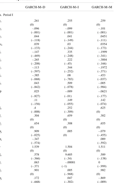
GARCH-M+D GARCH-M+I GARCH-M+M
A. Period I 1 .261 .255 .259 (0) (0) (0) 2 –.096 –.099 –.101 (–.001) (–.001) (–.001) 3 .044 .041 .0451 (–.118) (–.149) (–.111) 4 .039 .03 .0354 (–.133) (–.244) (–.173) 1 –.147 .335 –.1999 (–.469) (–.248) (–.341) 2 –.265 .222 –.3004 (–.208) (–.45) (–.166) 3 –.113 .344 –.1972 (–.597) (–.252) (–.371) 4 –.385 .08 –.453 (–.068) (–.783) (–.037) 5 .043 .509 –.005 (–.842) (–.078) (–.984) .025 –.009 –.0621 φ (–.827) (–.01) (–.177) .11 .149 .142 (–.156) (–.055) (–.074) 0 .4 .252 .625 (–.008) (–.309) (0) 1 .304 .659 .302 (0) (0) (0) 2 .654 .308 .655 (0) (0) (0) Qp .909 .005 –.079 (–.025) (0) (–.455) Qn –.347 .089 (–.574) (–.592) 1.539 1.504 1.511 (0) (0) (0) 0 .578 9.605 .589 (–.366) (–.34) (–.138) 1 .063 –.00001 0 (–.371 (–1) (–.999) 2 .901 .005 .982 (0) (–.968) (0) Qp .172 .047 –.869 (–.668) (–.302) (–.009)
TABLE 3. (Continued) Skewness .025 .008 –.009 Kurtosis 4.065 4.335 (4.272) JB Normality 69.049 108.143 98.235 L–Box Q(8) 18.055 15.277 18.329. (–.114) (–.227) (–.106) Q(18) 2.587 17.109 2.324 (–.301) (–.516) (–.315) Q(24) 23.425 21.284 23.318 (–.495) (–.622) (–.501) Q(30) 31.522 3.198 31.103 (–.39) (–.455) (–.41) Q(36) 5.584 47.961 49.786 (–.054) (–.088) (–.063) ARCH–LM(5) 2.665 2.642 2.227 (–.752) (–.755) (–.817) (10) 8.671 8.905 7.989 (–.564) (–.541) (–.63) (20) 22.953 22.162 19.124 (–.291) (–.332) (–.514) (30) 27.389 25.514 22.548 (–.603) (–.699) (–.833) (45) 5.464 46.125 42.124 (–.266) (–.425) (–.594) Sign bias –.375 –.759 –.601 Negative size 1.067 .687 .828 Positive size –1.135 –1.311 –1.218 Joint tests .878 .854 .826 Function Value –3435.266 –3434.2 –3437.17 Exclusion Test 6.608 8.749 2.806 B. Period II 1 .389 .48 .376 (0) (0) (0) 2 –.185 –.171 –.118 (–.045) (–.035) (–.107) 1 1.414 4.34 –.786 (–.565) (–.875) (–.585) 2 1.035 4.019 –.503 (–.671) (–.884) (–.766) 3 1.708 5.157 .118 (–.518) (–.852) (–.946) 4 1.618 5.022 .694 (–.41) (–.856) (–.647) 5 .561 4.272 –.327
TABLE 3. (Continued) (–.805) (–.877) (–.849) .121 .006 .271 φ (–.315) (–.889) (–.33) –.362 –1.405 –.052 (–.558) (–.869) (–.895) Qn –.421 .431 (–.287) (–.306) 7.573 2.169 3.589 (–.121) (0) (–.012) Skewness –.109 –.033 –.001 Kurtosis 2.004 2.518 1.979 JB Normality 6.417 1.461 6.429 L–Box Q(8) 6.794 6.103 7.038 (–.871) (–.911) (–.855) Q(18) 19.813 14.699 16.702 (–.343) (–.683) (–.544) Q(24) 21.121 15.824 19.101 (–.632) (–.894) (–.747) Q(30) 29.697 24.784 27.319 (–.481) (–.736) (–.606) Q(36) 38.227 32.045 37.594 (–.369) (–.657) (–.396) ARCH–LM(5) 4.623 5.69 6.684 (–.464) (–.338) (–.245) (10) 8.685 8.919 9.092 (–.562) (–.539) (–.523) (20) 16.134 19.263 15.228 (–.708) (–.505) (–.763) (30) 23.237 29.643 19.754 (–.805) (–.484) (–.923) (45) 42.422 5.706 34.616 (–.582) (–.259) (–.869) Sign bias –.267 –.759 –.724 Negative size –.309 .687 .253 Positive size –.174 –1.311 –1.335 Joint tests .042 .854 .616 Function Value –397.45 –41.484 –395.737 Exclusion Test 2.556 28.622 6.87 C. Period III 1 –.005 –.069 .012 (–.936) (–.199) (–.904) 2 .0854 .024 .047 (–.155) (–.652) (–.658)
variables. Therefore, variability of conditional standard deviations can be modeled better by incorporating additional information revealed by macroeconomic variables to capture the volatility better. Furthermore, ISE as an emerging stock market, is known to be sensitive to changes in macroeconomic variables (Muradoglu and Onkal, 1992; Muradoglu and Metin, 1996). Therefore these variables should also be included into the stock return equation. This inclusion will allow us to observe which variable has explanatory power on the behaviour of the conditional mean as well as the conditional variance.
TABLE 3. (Continued) (10) 6.236 9.351 7.997 (–.795) (–.499) (–.629) (20) 17.403 13.117 22.162 (–.627) (–.872) (–.332) (30) 21.322 18.987 26.479 (–.878) (–.94) (–.651) (45) 33.818 26.246 41.552 (–.889) (–.989) (–.619) Sign bias –.234 –.03 –.83 Negative size –.108 .364 .107 Positive size .267 .179 –.299 Joint tests .104 .115 .429 Function Value 398.431 -397.633 –396.976 Exclusion Test 6.302 7.899 9.212
Note: Results reported in table 3 Panel A, B, and C are obtained from the joint estimation of equation 6 and 7 for the exogenous variables namely, the price change of the US dollar in terms of TL (D), interest rates (I) and currency in circulation (M) in each time. and are the positive and negative values the depreciation and money
, ,
t t t
D+ D− M+ Mt
−
growth figures in absolute value. 1- 4 coefficients refer to the AR equation for the mean., 1- 5 coefficients are the day of the week effects, is the coefficient on the ARCHin -mean term, 0 is the constant in the conditional variance equation, 1 is the coefficient of one period lagged conditional variance, 2 is the coefficient of one period lagged squared residuals, i are coefficients on the exogenous variables for the mean respectively, Qp and
Qn coefficients are on the exogenous variables in the variance when the variable takes the
positive and negative values respectivel and finally is the scale parameter for the GED. The test statistics reported in table 3 are the Jarque-Bera normality test 2(2) for normalized residuals, the Ljung-Box Q-test for serial correlation in squared normalized residuals, ARCH-LM test of no AutoRegressive Conditional Heteroskedastic (ARCH) versus ARCH in normalized residuals and finally sign and size bias non-parametric test. (.) indicates the level of significance for the test statistics.
14. We also determined the order of the autoregressive process by the Schwartz (1978) criteria and included up to two lags of each of the macroeconomic variables. The results, not reported here, are robust with the results presented in table 3.
Table 3 reports the GARCH-M specifications described in equations 6 and 7.
The order of the autoregressive process is shorter during the crisis. It is two for period 2, and four for periods 1 and 3.14 During Period 1
(before crisis) the US dollar (Dt) and interest rates (It) have predictive power in explaining the behavior of the conditional variance. This result suggests that the depreciation of the exchange rate, and higher interest rates as important indicators of political and economic instability, increase volatility in the stock market. Moreover, there is a negative and statistically significant relationship between interest rates (It) and the
stock returns during this period, possibly due to their being close substitutes (Muradoglu, 1992). During this period the GARCH-M model also displayed a positive relationship between the conditional standard deviation and stock returns although the significance level of the estimated parameter is less than 10 percent.
During the crisis (period 2), none of the variables have a statistically significant coefficient in the conditional variance equation. Also, for the stock return equation, none of the macroeconomic variables have predictive power. The notable result for the crisis period is the negative coefficient of the conditional standard deviation in the mean equation, when the depreciation of US dollar (Dt), is used as a variable in estimating the conditional variance. As Poon and Taylor (1992) noted, when returns are lower than the average, speculative activity might have been induced and market volatility might have increased, leading to a negative relationship between risk and return. Ozer and Yamak (1992) have also shown a similar relationship between risk and return at ISE during the Gulf Crisis.
During Period 3 (after the crisis), only the money growth rate, (Mt ),
and depreciation of US dollar (Dt) have predictive power in the conditional variance equations. Unlike the negative coefficient of the depreciation variable (Dt) during the crisis period, the estimated
coefficient of Dt has a positive sign after the crisis. The positive effect
of Dt on conditional variability after the crisis indicates that higher depreciation increase the risks in the stock market. Similar to the period
before the crisis (period 1), after the crisis, during period 3, the interest rate (It) also has a negative coefficient in the stock return equation.
Besides there is a positive relationship between the conditional standard deviation estimated using Dt and stock returns.
VII. Discussions
In this study, we examined the risk return relationship during a financial crisis. Changes in the determinants of risk as well as the relationship between risk and stock returns before, during and after the financial crisis of 1994 in ISE are investigated by using the GARCH-M model. In this process, we first modeled risk and then considered the relationship between risk and return. Next, we examined the possible macroeconomic determinants of risk in the stock market as well as testing for their conceivable effects on stock returns.
The results indicate that first, for all sub-periods risk can be modeled by a GARCH(1,1)-M specification. However, risk, as represented by the conditional standard deviation, affects stock returns only during the crisis. Secondly, the relationship between macroeconomic variables and risk and risk-return relationships change as the economy progresses through different stages.
Before the crisis, the rate of change in the price of the US dollar in terms of Turkish lira and higher interest rates as indicators of political and economic instability and higher expected inflation respectively, increase the volatility in the stock market. However, we observe that during the crisis period, none of the macro-economic variables enter the variance equation. Since the 1994 funding crisis (Ozatay, 1996) emerged as a consequence of debt mismanagement, the government had to decrease the money supply, considerably during the crisis. After the crisis, as was the case before the crisis, higher interest rates increased volatility in the stock market. During this period, government-induced risk is also evident and the money growth variable enters the mean equation with a positive sign. This indicates that during the recovery period, expansionary, rather than contractionary monetary policy is positively associated with risk in the stock market.
The relationship between risk and stock returns becomes negative during the crisis period. Under normal conditions, the positive
15. See table 1, row 3 for the unconditional standard errors before, during and after the crisis.
relationship between expected returns and expected volatility indicates that equity risk premiums provide compensation for risk when volatility increases. However, during the crisis, as suggested by Poon and Taylor (1992), speculative activity might have been induced and market volatility have increased almost thirteen times,15 leading to a negative
relationship between risk and return. After the crisis, a positive risk-return relationship is reestablished and this can be interpreted as a sign of recovery from the effects of the crisis.
Besides risk, macroeconomic variables that explain the behavior of stock returns also change before, during and after the crisis. Like other researchers (Fama and Schwert, 1977; Solnik, 1983), we also find a negative relationship between interest rates that proxy for expected inflation and stock returns before the crisis. Our study adds to the literature by showing that none of the macroeconomic variables have predictive power during the crisis period. After the crisis, similar to the period before the crisis, the interest rate enters the stock return equation with the expected sign.
VIII. Conclusions
This study attempts to make three contributions to the field. First, it specifies the conditional variance equation including macro-economic variables, relevant information set for emerging economies that is often overlooked in various GARCH specifications. Risk, in this paper, is shown to have macro-economic determinants. This is the case for asset returns as well. Second, we employ the GARCH-M methodology to investigate asset returns and conditional volatilities during a major financial crisis in an emerging market, a setting that is often ignored in the financial literature. In this study we observe that during a financial crisis, risk-return relationship and the factors that determine risks in stock markets change. This is important in emerging markets because the appropriate cost of capital used to evaluate foreign direct or portfolio investments will change and so will international asset allocation decisions. GARCH (1,1), which is known to be an appropriate specification for modeling mature markets, proves to capture volatility
16. We would like to thank an anonymous referee for raising the issue.
and stock returns successfully in an emerging market and under different economic conditions including a crisis period. Third, this study attempts to offer possible explanations to the mixed results of previous research, as it is shown that in the periods before, during, and after a major financial crisis, determinants of risk as well as the risk return relationship change depending upon the state of the economy.
This paper might be noticed as a case to help us understand better financial crisis in emerging markets. The worldwide crisis in 1998 that was stimulated with a crisis in an emerging economy Korea, showed that neither the academics, not the practitioners were well prepared to comprehend the various dimensions of crisis in emerging economies. Therefore, neither international investors, nor international agencies, nor governments were well prepared to react appropriately and instantaneously to crisis in emerging economies before the crisis was epidemic.
International portfolio managers have difficulty in dealing with financial crisis in emerging markets. Reasons are several. Country specific factors are not always easy to analyze and interpret quickly. Overreaction is a widespread phenomenon in investment decisions in general and during crisis in particular. Compared to firm specific information, macroeconomic variables are relatively easy to follow and interpret for international portfolio managers. They also constitute an important set of information due to the overwhelming role of state in economic activity. In this study we show, the international investor that during financial crisis the risk-return relationships and the determinants of risk change. Accordingly, international investors should adjust the cost of capital used in evaluating investments in individual stock markets and thus their international asset allocation decisions.
Clearly, a lot more needs to be done in this area. Further research is expected to concentrate in three major avenues. First, other country studies are definitely needed to understand the relationship between macro-economic variables and risk in financial markets. Second, conditional variances of macro-economic variables can be used to estimate conditional variance of stock returns.16 This specification would
enable us to investigate the effect of risk in general economic conditions on risk in stock returns.
Third, due to the increased integration of world markets, volatility spillovers need to be investigated. Macro-economic variables constitute appropriate information set in this framework as well, as they are easily accessible by the international investor.
References
Ajayi, R.A. and M Mougoue, Dynamic relations between stock prices and exchange rates, The Journal of Financial Research, 19(2), 193-207. Andrews, K.W.K, 1993, Tests for parameter instability and structural change
with unknown change point, Econometrica, 61, 821-826.
Assoe, K.G., 1998, Regime switching in emerging stock market returns, Multinational Finance Journal, 2, 101-132.
Attanasio, O.P. and S. Wadhwani, 1989, Risk: Gordon’s Growth model and the predictability of stock market returns, Stanford Center for Economic Policy Research Discussion Paper Series:161,47.
Baillie, R.T. and R.P. DeGennaro, 1990, Stock return and volatility, Journal of Financial and Quantitative Analysis, 25, 203-215.
Bakir, H. and B.H.Candemir, 1997, Menkul kiymet getirilerinin sartli varyans modelleri: IMKB icin bir uygulama in Doc. Dr. Yaman Asikoglu’na Armagan, (Capital Market Board Publication, No:56, Pelin Ofset, LTD, Ankara).
Balaban, E., H.B. Candemir and K. Kunter, 1997, Istanbul menkul kiymetler borsasinda yari-guclu etkinlik, in Doc. Dr. Yaman Asikoglu’na Armagan, (Capital Market Board Publication, No:56, Pelin Ofset, LTD, Ankara). Balaban, E. and K. Kunter,1997, A note on the efficiency of financial markets in
a developing country, Applied Economic Letters, 4, 109-112.
Bekaert, G. and C.R. Harvey, 1997, Emerging equity market volatility, Journal of Financial Economics, 43, 29-77.
Bollerslev, T.1986, Generalized autoregressive conditional heteroscedasticity, Journal of Econometrics, 31, 307-327.
Bollerslev, T., Y.R.Chou, and F.K. Kroner, 1992, ARCH modeling in finance, a review of the theory and empirical evidence, Journal of Econometrics, 52, 5-59.
Bollerslev, T., R.F. Engle, and M. Wooldridge, 1988, A capital asset pricing model with time varying covariances, Journal of Political Economy, 96, 116-131.
Boratav, K., O.Turel, and E.Yeldan,1996, The macroeconomic adjustment in Turkey,1981-1992 : a decomposition exercise, Yapi Kredi Economic Review, 7, 3-20.
to financial market prices, Journal of Econometrics, 72, 33-48.
Chow, G.C. 1960, Tests of equality between sets of coefficients in two linear regressions, Econometrica, 52, 211-222.
Engle, R. F. 1993, Statistical models for financial volatility, Financial Analysts Journal, 1, 72-78.
Engle, R.F., R.M. Lilien, and R.P.Robins, 1987, Estimating time varying risk premia in the term structure: the ARCH-M model, Econometrica, 55, 391-407.
Errunza, V., K. Hogan, O. Kini and P. Padmanabhan, 1994, Conditional heteroskedasticity and global stock return distributions, The Financial Review, 29, 8, 293-317.
Fama, E. and G.W. Schwert, 1977, Asset returns and inflation, Journal of Financial Economics, 5, 115-146.
French, K.R., G.W. Schwert and R.F. Stambaugh, 1987, Expected stock returns and volatility, Journal of Financial Economics, 19, 3-30.
Friedman, M. 1968, The role of monetary policy, American Economic Review, 58, 1-17.
Geske, R. and R. Roll, 1983, The fiscal and monetray linkage between stock returns and inflation, The Journal of Finance, 38, 1-32.
Glosten, L.R., R. Jagannathan and D. Runkle, 1993, On the relation between the expected value and the volatility of the nominal excess return on stocks, The Journal of Finance, 48/5, 1779-1801.
Ghysels, E. and R. Garcia, 1996, Structural change and asset pricing in emerging markets, Working Paper, #34, CIRANO, University of Montreal.
Griffiths, W., R.C. Hill, and G.G. Judge, (1993), Learning and Practicing Econometrics, John Wiley and Sons, Canada.
Gultekin, N.B., 1983, Stock market returns and inflation: Evidence from other countries, The Journal of Finance, 38, 49-65.
Harvey, Campell R.1995, Predictable risk and returns in emerging markets, Review of Financial Studies, 8, 773-816.
Im, B. and S. Kim, 1998, Regulatory Reform Policy of Financial Services industry in Korea, paper presented at the Western Economic Association International at Pacific Rim Conference in Bangkok, Thailand, January. Hamao, Y., R.W. Masulis and V. Ng, 1990, Correlations in price changes and
volatility across international markets, Review of Financial Studies, 3, 281-307.
Jarque, C.M. and A.K. Bera, 1980, Efficient tests for normality, homoscedasticity, and serial independence of regression residuals, Economics Letters, 6, 255-259.
Kaminsky, G.L. and C.M. Reinhart, 2000, On crisis, contagion, and confusion, Journal of International Economics, 51, 145-168.
Kendall, J.D. and A. McDonald, 1989, Univariate GARCH-M and the risk premium in a foreign exchange market, unpublished manuscript (Department
of Economics, University of Tasmania, Hobart).
Lintner, J, 1965, The valuation of risk assets and the selection of risky investments in stock portfolios and capital budgets, The Review of Economics and Statistics, February, 13-37.
Ljung , G.M. and G.E.P. Box, 1978, On a measure of lack of fit in time series models, Biometrica, 65, 297-303.
Malliaropulos, D., 1998, International stock return differentials and real exchange rates, Journal of International Money and Finance, 17, 493-511. Metin, K., 1995, The analysis of inflation : the case of Turkey (1948-1988), (Capital Market Board of Turkey : Publication Number 20, Ankara, Nurol Publishing Co).
Mishkin, F.S, 1982, Does anticipated monetary policy matter? An econometric investigation, Journal of Political Economy, 90, 22-51.
Muradoglu, G., 1992, Factors influencing demand for stocks by individual investors, Proceedings of Izmir Iktisat Kongresi, Vol.1.
Muradoglu, G., 2000, Efficiency and anomalies in the Turkish stock market, in Security Market Imperfections in Worldwide Equity Markets, ed. Keim, D., Ziemba, W., Cambridge University Press, 364-390.
Muradoglu, G. and K. Metin, 1996, Efficiency of the Turkish stock exchange with respect to monetary variables: a cointegration analysis, European Journal of Operational Research, 90, 555-576.
Muradoglu, G. and D. Onkal, 1992, Semi-strong form of efficiency in the Turkish stock market, METU Studies in Development, 19(2), 197-208.
Muradoglu, G. and M. Unal, 1994, Weak form efficiency in the thinly traded Istanbul securities exchange, The Middle East Business and Economic Review, 6, 37-44.
Ozer, B. and S. Yamak, 1992, Effect of Gulf crisis on risk return relationship and volatility of stocks in Istanbul stock exchange, METU Studies in Development, 19(2),209-224.
Ozatay, F, 1996, The lessons from the 1994 crisis in Turkey: public debt (mis)management and confidence crisis, Yapi Kredi Economic Review, 7(1), 21-38.
Pagan, A. and A. Ullah, 1988, The econometric analysis of a model with risk terms, Journal of Applied Econometrics, 3, 87-105.
Pettinen, A., Devaluation, risk related peso problems in stock returns, International Financial Markets Institutions and Money, 10(2) 181-197. Poon, S. and S.J.Taylor, 1992, Stock returns and volatility: an empirical study
of the UK stock market, Journal of Banking and Finance, 16, 37-59. Ross, S.A., 1976, The arbitrage theory of capital asset pricing, Journal of
Economic Theory, 13, 341-360.
Schwarz, G, 1978, Estimating the Dimension of a Model, The Annals of Statistics, 6, 461-464.
conditions of market risk, The Journal of Finance, 19, 425-442.
Solnik, B. 1983, The relation between stock prices and inflationary expectations: The international evidence, The Journal of Finance, 38, 35-48. Theodossiou, P., E. Kahya, G. Koutmos and A. Christofi, 1997, Volatility
revision and correlation of returns in major international stock markets, The Financial Review, 32, 205-224.