Portfolio selection methods: An Application to İstanbul Securities Exchange

POETFOLIO SELECTION Μ Ε ΊΉ 0Ο 3

¿ л Р р Т ;і'ТТ/'Ѵ К'‘ .-nj г··. •rrv^J/»n » ЧѴ.".·_{á. \ J i b lA í'^ ; Л>} ■ S ? O é fS J,e> l ù ê B O i O '5 o ΓΌΕ'’"*"”·

D a te Prin ted ; February 27, 1989

PORTFOLIO SELECTION METHODS :

AN APPLICATION TO ISTANBUL SECURITIES

EXCHANGE

A THESIS

SUBMITTED TO THE DEPARTMENT OF MANAGEMENT AND THE GRADUATE SCHOOL OF BUSINESS ADMINISTRATION

OF BILKENT UNIVERSITY

IN PARTIAL FULFILLMENT OF THE REQUIREMENTS FOR THE DEGREE OF

MASTER OF BUSINESS ADMINISTRATION

./· 71 t T T

By

i. Tunç Seler

February 1989

anC 'Sal('r . J l ,

Hü

5 7

СКс

_{. 5}

, S 4 5 і э г з 0 . . 1 s * f»

I certify that I have read this thesis and that in my opinion it is fully adequate, in scope and in quality, as a thesis for the degree of Master of Business Adminis­ tration.

Assistant Prof. Dr. Kiir§at Aydogan(Principal Advisor)

I certify that I have read this thesis and th at in my opinion it is fully adequate, in scope and in quality, as a thesis for the degree of Master of Business Adminis­ tration.

Assistajit Prof. Dr. Erdal Erel

I certify that I have read this thesis and that in my opinion it is fully adequate, in scope and in quality, as a thesis for the degree of Master of Business Adminis­ tration.

Approved for the Graduate School of Business Administration :

a

L ·

U u.. A

___________-Prof. Dr. Sim dey 'Kgan, Director of Graduate School of Business Administration

ABSTRACT

PORTFOLIO SELECTION METHODS :

A

n a p p l i c a t i o n t o

İ

s t a n b u l s e c u r i t i e s e x c h a n g e

i. Tunç Seler

Master of Business Administration in Management

Supervisor: Assistant Prof. Dr. Kürşat Aydogaii

February 1989

In this study, Modern Portfolio Theory tools -are used for constructing efficient portfolios. The Markowitz mean-variance model and Sharpe single index model are presented and calculated, for the construction of efficient portfolios from the Istanbul Securities Exchanges’ first market slocks for the 1986 - 1987 period. Constructed efficient portfolios are compared on the risk and return scales.

K e y w o rd s : Portfolio, Efficient Frontier, Diversification, R eturn, Risk, Capital Markets, M athematical Programming Structure.

Ö ZET :

Portföy Seçim Yöntemleri :

İstanbul Menkul Kıymetler Borsası İçin Bit Uygulama

i. Tunç S eler

İşletme Yönetimi Yüksek Lisatıs

Tez Yöneticisi : Kürşat Aydoğan

Şubat 1989

Bu çalışmada Modern Portföy Teorisi araçları , Etkinlik Siniri oluşturulması için kullanılmıştır. Markowitz ortalama varyans modeli ve Sharpe tekli index modeli açıklanmış ve 1986 - İ987 dönemi için, İstanbul Menkul Kıymetler Borsası birinci pazar hisse senetleri için hesaplanmıştır. Elde edilen etkinlik öncüleri risk ve getiri boyutlarında karşılaştırılmıştır.

A n a h ta r K e lim e le r : Portföy, Etkinlik Sının , Çeşitlendirme, Getiri , Risk , Sermaye Piyasaları , Matematiksel Programlama Yapısı.

ACKNOWLEDGEMENT

I would like to thank to my thesis supervisor Assistant Prof. Dr. Kürşat Aydogan for his guidance and patiance through out this study. Assistant Prof. Dr. Erdal Erel and Assistant Prof. Dr. Gökhan Çapoğlu also made valuable comments on the structure of the text.

I also would like to thank to Ercan Erkul for his valuable comments and for the time he spent with me for discussions. İzzet Perçinler, also made very valuable comments,.and was very kind in helping as a perfect proofreader. I will take credit for all possible errors.

I have to express my thanks to my parents, who always supported me.

I would also thank to all collagues that helped-for various items through out this study.

TABLE OF CONTENTS

1 IN T R O D U C T IO N : 1

1.1 Financial Markets ; ... 1

1.2 Turkish Financial System ; ...'... 3

1.2.1 Turkish Securities Markets : ... 3

1.3 Istanbul Securities Exchange : ... ... 5

1.3.1 IMKD Index : ... ... C 1.3.2 Return Index : ... ... . 7

1.4 Investing in Equity Markets : ... 7

2 Li t e r a t u r e r e v i e w : lo 2.1 Mean - Variance portfolio selection method : 10

2.2 Sharpe - Single Index Method ; ... 11

2.3 Other Methods : ... 12

3 M E T H O D O L O G Y : 14 3.1 Formulation : ... 15

3.1.1 General relationships and definitions : ... 15

3.1.2 Mean - Variance model : ... 17

3.1.3 Single Index Model ; ... 21

3.2 Assumptions of the Study : ... 25

3.2.1 Mean - Variance Model : ... 25

3.2.2 Single Index Model : ... 2G 4 H A i’A Î 27 5 F IN D IN G S O F TFIE S T U D Y A N D C O N C L U S IO N S î 32 5.1 Mean - Variance Model : ... 32

5.2 Single Index Model : ... 34

5.3 Conclusions : ... T.! 5.3.1 Findings : ... 42

LIST OF FIGURES

1.1 İMKB index values during Jan. 1986 - Dec. 1987 G

1.2 IMKB index returns versus Return index values duriiig January 1986

to December 1987 ... 7

3.1 Efficient F r o n t i e r ... 18

5.1 Efficient Frontier under the Markowitz m o d e l... 32

5.2 Efficient Frontier’s Risk preferance graph ... 33

5.3 Efficient Frontier’s Iteration Summary g r a p h ... 34

5.4 Efficient Frontier’s Basic variable summary graph 36 5.5 MVP combination under the Markowitz m o d e l ... 36

5.6 Efficient Frontier under the Single Index m o d e l ... 37

5.7 SİM portfolio beta versus Lambda coefficient... 39

5.8

SiM

alpha and beta values compared... 4.0 5.9 MVP combination under the SIM model ... 40

LIST OF TABLES

1.1 Public and Private sectors’ relative percentages in primary markets. 3 1.2 Yearly percent changes in primary market transactions during 1984,

to 1987 ... , ... 4

1.3 Incentives granted to investors ... 5

4.1 List of Stocks’ analyzed... ... 29

4.2 Regression results for IMKB index R e t u r n s ... 30

4.3 Regression results for Return index Returns ... 31

5.1 Markowitz model Efficient Frontier p ro p e rtie s... 35

5.2 Portfolio Alpha and Beta under the Single Index m o d e l ... 38

NOMENCLATURE :

The notation used In this study is presented below.

Bi B , C i d i,t Ei Ep l i X i B i.n P i p3,r R i n,e R j R p R p R i m n A X { 2 rn 2 P a a o ^P

Alpha coefficient of the asset. Portfolio Alpha .

Beta coefficient for the asset. Portfolio Beta .

The error term.

Dividend and other payments for the asset on the i ‘’' period. Expected return of the asset.

Expected rate of return on the portfolio. The market index.

Proportion to invest form the asset. Price of asset on the period . Price of old quotation on the period.

Price of the stock split right owning quotation. Average rate of return on the asset.

R ate of return on the asset on the period. Riskfree rate of return.

Average Portfolio Return. Portfolio rate of return.

Rate of return on the asset.

Number of stocks to be received as the result of the stock split. Number of periods.

Risk preferance coefficient.

Proportion to invest on the asset. Standaxt error of the estimator. Variance of the market index. Portfolio Variance.

Covariance between and assets’ returns. Portfolio Standart Deviation.

Beta value of the security.

1. INTRODUCTION :

The purpose of this study is the construction of efficient portfolios by using stocks listed in Istanbul Securities Exchange . In this study, Markowitz full covariance model and Sharpe’s single index model are utilized for the construction of efficient portfolios. The constructed efficient portfolios are compared on the risk and return spaces and policy recomendations for investors are put forward as a result of this study.

1.1

F in a n cia l M arkets :

Financial markets have significant impacts on economic systems, because of their vital economic functions. The function of financial markets is to provide a conve­ nient medium for savings to be done and investments to be realized. Another major function of financial markets is the creation of new wealth by providing a connection between sa.vings and investments. Wealth can be defined as the summation of real and financial assets minus liabilities or net worth plus liabilities.

Although financial markets can create new wealth, a great portion of the transac­ tions th at takes place in these markets have no effect on the creation of new wealth. This can better be seen in the markets for corporate debt and markets for corporate equity. The transactions in these mArkets, only affect the ownership of liabilities. However, wealth,can be created in these markets by issuing new stocks or debt.

Financial markets can be analyzed under two major submarkets. These submarkets are money markets and capital markets.

Financial markets classification : 1. Money markets .

2. Capital Markets .

2.1 markets for goverment securities 2.2 markets for local goverment securities 2.3 mortgage markets

2.4 markets for corporate debt 2.5 markets for corporate equity

Capital markets have certain distinguishing properties. These are;

1. having a maturity of one year or more 2. being both a wholesale and retail market

There are primary and secondary markets which carry out the operations for trans­ actions in financial markets. Securities that are available for the first time arfe offered through the primary markets. This is im portant beca.use, primary markets create new funds for the issuers. After their purchase in primary markets, secu­ rities are traded in the Secondary markets. Secondary markets have two ma.jor segments. Those are the organized exchanges and over-the-counter markets. Orga­ nized exchanges are physical market places where auction can take place between the representatives of the buyers and sellers. Over-the-counter market is not a phys­ ical market. The securities that are traded in the-over-the-counter markets are the unlisted securities. This market can be characterized by a network of buyers and sellers over a country, connected by communication links for negotiating the buying or selling prices.

The market for corporate debt can be further divided into two submarkets accord­ ing to their organizational structures. The.se are :

1. organized security exchanges

2. over-the-counter markets or over-the-telephone markets.

1.2

T urkish F inancial S y stem :

The Turkish financial system is dominated by commercial banks. The extensive power and the domination of commercial banks in the Turkish financial system is due to the legislators concern for the protection of the investors [29] .

Another feature of the Turkish financial system is the goverment’s entering to the financial markets to finance the budget deficits..

1.2.1

T urkish S ecurities M arkets :

S u p p ly Side :

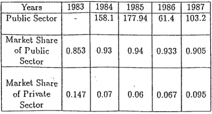
The public sector securities dominates the supply side of the market. This can be seen in Table 1.1 [8] as percent increase and relative market share during 1983 to 1987. Public sector market share in the primary market has been over 85 % for the last five years, which indicates a domination in the new issues market.

Years 1983 1984 1985 1986 1987 Public Sector - 158.1 l'77.94 61.4 103.2 Market Share of Public Sector 0.853 0.93 0.94 0.933 0.905 Market Share of Private Sector 0.147 0.07 0.06 0.067 0.095

In the corporate sector, there is a reluctance for changing its financing behavior. Corporate sector depends heavily on. bank financing. This reluctance of the corpo­ rate sector is closely related with the small size of financial markets in Turkey. However, there is a recent growth in the corporate sector’s bond issues. The recent tendencies of the corporate sector to finance its activities through security markets, is a direct result of the change in the behavior of the banks. Banks do advice cor­ porations to issue securities and particularly bonds, to finance their operations.

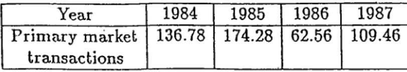
The yearly percent changes in the primary market transactions according to the previous year is presented in Table 1.2 [8] . These figures include both the public and private primary market issues that arc allowed by the Capital Markets Board.

Year 1984 1985 1986 1987

Prim ary market transactions

136.78 174.28 62.56 109.46

Table 1.2; Yearly percent changes in primary market transactions during 1984 to 1987

Dem anci Side t

To flourish the level of demand in securities markets, certain tax incentives are granted to individual investors. Those lax incentives are presented in Table 1.3, for the individual and collective portfolios [29] . These incentives remained the same up to January 1989 together with one new rule. The interest income for the corpo­ rations obtained from the securities will be taxed according to this new application and the taxation will be % 10. The concept of Collective portfolio in the Table 1.3, in general terms refers to mutual funds.

To flourish the level of demand, the double taxation of dividends is also prevented. Corporate tax oecomes the final tax bn these earnings. Capital gains becomes taxfree, if and only if, the security in question is listed on an exchange or sold through licensed intermediary agencies.

The changes in the demand side of the market have been slow. Individual investors react rather slowly in investing their savings on a group of totally new, hence un­ known instruments. Institutional investors in Turkey are practically non-existent in

T ax Incentive Individual portfolio Collective portfolio Bank deposits

Shares

Corporate bonds

Profit Loss Sharing Cert. Bank Bills Finance bills F shares T-Bills Goverment Bonds Revenue Sharing C.____ 10.4 % withholding tax Tax exempt 10.4 % withholding tax 10.4 % withholding tax 10.4 % withholding tax 10.4 % withholding tax Tax exempt Tax exempt Tax exempt Tax exempt

ca.n not deposit Ta.x exempt Tax exempt Tax exempt can not deposit Tax exempt can not deposit Tax exempt Tax exempt Tax exempt

Table 1.3: Incentives granted to investors

the capital markets. Institutional investors are corporations which collect funds for investing. In Turkey, Social Security Board and Insurance corporations can be given as examples for institutional investors. However their rules in the capital markets have been limited so far [29].

1.3

İsta n b u l S ecu rities E xchange :

İstanbul Securities Exchange {tsianhul Menkul Kıymetler Borsası ) started op­ eration in January 1986. Stocks are traded in these markets according to their transaction volumes in the exchange. The organization of the İstanbul securities exchange can be analyzed under two headings :

1. F irst Market , {Birinci Piyasa ) Second Market , ( İkinci Piyasa )

IMKB Index V aines

1.3.1

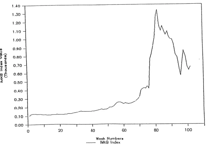
Figure 1.1: IMKB index values during Jan. 1986 - Dec. 1987

IMKB Index :

The IMKB index is an average of the stock prices, weighted with the corporate capital amounts and dividend payments. The IMKB index is calculated for the first 43 stocks that were traded in the first market in January 1986. January 1986 is taken as the base period (January 1986 = 100 ) for this index.

iMKB index values are presented in Figure 1.1 during the January 1986 - December 1987 period [18]. This makes a times series consisting of 102 weekly observations.

IMKB Index v ersu s R eturn Index

R c lu rn F ig u re s c ro s s plo t

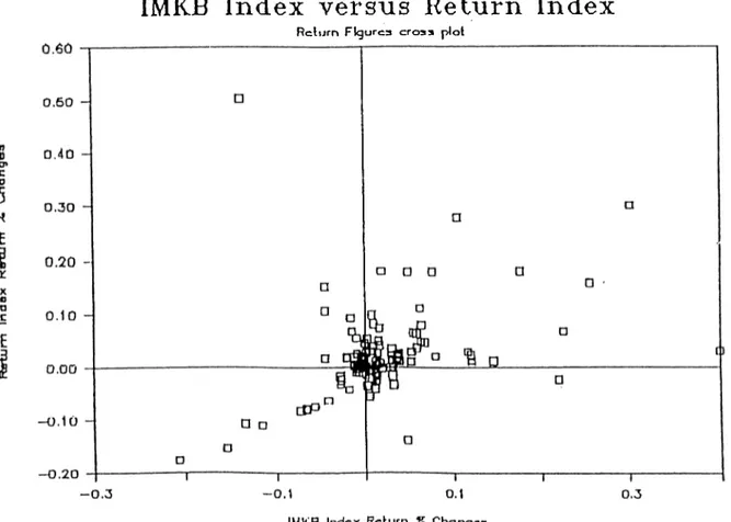
Figure 1.2: IMKB index returns versus Return index values during January 1986 to December 1987

1.3.2 Return Index :

To measure the return trends in the Istanbul securities exchange, another index is developed and used in this study. This index is named as the Return index, which is constructed from the average returns for a given period.

The IMKB index returns and Return index are plotted against each other to present the different natures of the indexes and their potentials to show the actual return level in the m arket in Figure 1.2 . Since the Return index is an average of the returns, and if the IMKB index is argued to be showing the overall return level, then, a distribution around a 45° line >vould be expected. It can be concluded that IMKB index is not an appropriate measure for the applications th at utilize the market index concept, which measures the market’s price level.

1.4

In v e stin g in E qu ity M arkets :

Investment is a commitment of funds made in the expectation of some positive rate of return. Investment and speculation can be distinguished by the time horizon and

risk return characteristics.

Investments in equity markets can be realized by investing in common stocks of corporations. A common stock is a represantation of ownership for the firms. Com­ mon stocks have no m aturity date at which a fixed value will be realized like bonds and lOUs (I owe you). Investing in common stocks gives the voting right for the corporation’s decisions, and receiving earnings of the firm, as dividends .

R eturn from investing in common stocks is realized in two forms ;

1. Dividends, 2. Capital gains.

Dividends can be paid out by the decision of the board of directors of the corpora­ tions, if there are sufficient funds available for sUch an action. Capital gains is the difference between the buying price of stocks and price at fei specific time. It can be stated as , CG = P 2 - P j P i (1) where. P2 iselling price Pi ;buying price.

The possibility of high volatility in capital gains and dividends reqiiires the careful analysis of the stocks to be invested and traded. There are two approaches;

1. Traditional Investment Analysis, 2. Modern Security Analysis approaclies.

The Traditional approach is interested in the projection of prices and dividend amounts for forecasting the'future dividends and niarket value of the stocks. The projected amounts for prices and dividend amounts are discounted back to present and named as the intrinsic value. The comparison of the intrinsic value and com­ mon stock’s market value determines the buying or selling decision for stocks.

Modern security analysis approacli, on the other hand, is interested with the risk

return estimates of the common stocks. Generally two approaches can be applied. ' 8

These two approaches are ;

1. Fundamental analysis , 2. Technical analysis .

Fundamental analysis emphasizes the analysts should consider m ajor factors effect­

ing the economy, the industry, and the company in order to determine the invest­ ment decisions. Fundamentalists make a judgement of the stock’s value within a risk-return framework based upon earning power and economic environment. At any time, the price of a security is equal to the discounted value of the stream of in­ come for that security. Therefore the price of a security can be stated as a function of the anticipated returns plus the anticipated capitalization rates corresponding to future time periods.

Technical analysis approach to investment is essentially a reflection of the idea that

the stock market moves in trends which are determined by the changing attitudes of investors to a variety of economic, monetary, political and psychological forces. The objective of technical analysis is to identify changes in potential trends at an early stage and to maintain an investment posture [33] .

2. LITERATURE REVIEW :

The era of modern portfolio theory started with two papers published in 1952. These papers were from Roy and Markowitz.

Roy [34] defined the best portfolio with the probability of producing a rate of return below some desired level. If portfolio return is represented by 71,, and the desired level of return with R¿, then Roy’s formulation can be stated as, minPr(7?.p < R j).

The second major contribution to the modern portfolio theory was from Markowitz [23]. Markowitz proposed an objective portfolio selection criterion in his article. This criterion is known as the mean-variance portfolio selection method. Also, graphical mean-variance portfolio selection was presented by Markowitz in this ar­

ticle. in 1957, Markowitz presented the generalized solution methodology for the tnean-variance portfolio selection problem. [27]

2.1

IVieati - Variance portfolio selection method :

The mean-variance portfolio selection method uses mean and vatiance of returns for measures to capture and evaluate the relevant information about the opportunity set. The logic of the mean-variance portfolio selection method can be explained by the following postulates :

Let Ri denote the return on asset and cr,· denote the standart deviation of the return for the asset. Then for certain cases, investors’ decisions can be predeter­ mined according to the mean-variance criterion. Here the investors are assumed to be rational, who prefer more to less.

1. If the returns of two assets are equal, then investors will prefer the asset with lowet variance on return.

= R2 prefer minimum variance.

2. If the variances of two assets are equal, then investors will prefer the asset with the higher rate of return.

cTj = (72 —^ prefer maximum return.

The Markowitz model’s data requirement for an n security set is as follows ;

1. n return terms, 2. n variance terms,

3. covariance terms.

There is another measure which is required in this analysis, and th at is the investors risk preferance measure. This measure determines the relative importance of unit return compared with unit risk, from the investors point of view. This measure is named as the lam bda coefficient and used as A in this study.

As the risk preference coefficient, lambda ( A ) , will change fot A > 0, modicient portfolios, which are superior to all other combinations under mean-variance crite­ rion will be traced for that opportunity and constraint set.

Markowitz model when used for ex ante analysis has certain inconveniences. The user of this model should be able to predict the n return terms and should also be able to predict the n number of retutn variation coefficients for an n asset case. In addition to these predicitions, the analysts should predict covariance terms or serial correlation coefficients between assets or securities , which is very difficult and time consuming m ethod and infact practically is an impossible task. This property is the major drawback of the Markowitz mean-variance portfolio selection method.

2.2

Sharpe - Single Index Mfethdd :

In 1963, another approach to the portfolio selection problem was developed by Sharpe [30]. This approach was named as index models or Sharpe index models.

As tlie name implies, this models depend on indexes that measure the volatility in security markets. The logic of the index method can be explained as follows. The securities are affected by the overall fluctuations in markets. Generally some stocks are more sensitive to overall changes than others, and if so, then investors can forecast the fluctuations in stocks returns as a function of the overall market fluctuations. The measure used for this is named as the Beta coefiicient (^; or

B{ ). The stock price observations indicates that, the stock prices intend to move

together. The price fluctuations in markets are measured with an index which is an average of the stock returns, weighted with some other information content on the gain that was provided to the stock holders.

The Single index model utilizes this relationship between the market fluctuations and stock returns. Sharpe [30] defined the functional relatiohship between the m ar­ ket and stock returns in a linear functional form as it is presented in section 3.1.3 in equation ( 21 ) .

Index model uses return and variation of returns as a function of the securities responsiveness to the overall market fluctuations. As index models have certain computational efficiencies when compared with Markowitz inodel , index models became well known and applied.

The volatility measures are also different in these two models. The Markowitz model uses the standart deviation of return which is presented in section 3.1.1 and in equation ( 5 ) as the volatility measure where the index model uses the beta coefficient for this purpose which is presented in section 3.1.3 and in equation ( 21 ).

A brief emprical comparison of the Markowitz model and index models can be found in Cohen and Pogue [10], and a comparison of the index models with each other (Single index versus Multiple index models) can be found in Kwan [20] .

2.3

Other Methods :

There are various other a|>proache3 knd studies which utilize different techniques for the portfolio selection problem. Those studies utilize different types of assump­ tions and many of them are not as widely known and applied as the Index and Markowitz models. Some of the different assumption based studies are presented below for presenting a wider picture of the techniques used for the portfolio problem.

Jacobs [19] argued that the mean-variance and index models are only suitable for

the institutional investors’ portfolio selection process, with holding many number of securities with some in very small proportions. However, the situation that the small or non-institutional investors are facing is that, they are forced to select between the m utual fund shares and direct investments in a relatively small proportion from the securities. Jacobs proposed a mean-variance portfolio selection procedure with turn over constraints that would minimize the commisions to be paid and bring out a managable size for the small investors’ portfolio.

Faaland [15] formulated the portfolio selection problem with a quadratic integer programming structure. Faaland, in his article, presented a generalized version of the approacli that Jacobs used for the small investors. In this article computational summaries about CPU time and iterations can be found.

Another interesting portfolio selection method is presented by Canto [7]. The Fat CATS ( Capital Tax Sensitivity ) approacli is an encouraging approacli for the port­ folio selection problem for beating the market This approach considers macroe­ conomic shocks for the selection process.

Portfolio selection based on the price earnings ratio is another widely used method. British academicians Keown, Pin and Chen [9] used this approach for the British stock market. In that study the price earnings ratio based applications’ history and· performance records can also be found.

A review of the related literature on portfolio theory can determine the classes of problems that have been analyzed by the modern portfolio theory. These classes of problems are ;

1. Actual portfolio selection and money allocation based on mean-variance anal­ ysis. This application imposes complex constraints depending on the manage­ rial attitudes and legal constraints.

2. Economic analysis usage, the analysis of economy under the assumption that investors are acting upon mean-variance efficiency. The usage of the mean- Variance model for the economic analysis typically assumes highly simpli­ fied constraint sets. Such can be seen in the Tobin-Shafpe-Litner model and Black’s model.

'The term Dealing the Market refers earning higher returns then the market index returns.

3. METHODOLOGY !

In this study ex po^i data is used for the construction of efficient portfolios. The methods that are used in this normative study are the tools of the Modern Portfolio theory. The Markowitz and Single index models are briefly explained below.

The objective of the Portfolio Analysis is to determine the set of efficient portfolios or efficient frontiers [23]. Mathematically, that is to maximize expected return and minimize risk.

Four classes of calculation approaches can be utilized for the construction of the efficient frontier. These are :

1. Short selling allowed with riskless lending and borrowing; 2. Short selling allowed with no riskless lending and borrowing; 3. No short selling allowed with riskless lending and borrowing; 4. No short selling allowed with no riskless lending or borrowing.

Short selling process is a strategy that investors use when it is believed th at trading a security whiclx is non existing in the investors portfolio, can provide positive returns. Short selling or going in a short position for a security requires the selling of a non owning stock and then buying that stock for physical or electronic delivery, the price difference between selling knd buying; becomes the return for such a transaction. Selling of a non owning stock is generally supplying a security which is believed to decrease in price. Since one can provide the delivery of a stock sometime later, and during that period if the price of a security is believed to decrease, then an investor can go for a short position. Then the difference between the selling and buying prices becomes the positive return for the short seller, if the selling price is greater then the buying price.

In this study, riskless lending and borrowing with no short selling allowed approacli is utilized for the selection methods.

This can generally be formulated as ;

maxRp — Rj Subject to ; (1) R.p R j X{ ^ ^ d, t = l : Portfolio return. : Riskfree rate.

: Proportion to invest in the asset. : Portfolio standart deviation.

(2)

3.1

Formulation :

The formulation th at is used in this study to delineate efficient frontiers in Markowitz and SIM is presented below.

3.1.1

General relationships and definitions

1. R etu rn :

_ - -P,·,((_!) +

* ' | i P (3)

r,-_t ; Rate of return on the stock on the period.

Pi n ’■ Price of P^ asset on. the period .

di^i : Dividend .and other payments for the P^ asset on the P'* period.

2. Avet-age return :

Ri = E j= i n j

n

Ri : Average rate of return on the t"’ asset,

n : Number of periods.

(4)

3. V ariance o f R etu rn : , _ - RiY Ci = n — 1 cr? ; Variance of return for the asset.

(5)

4. Covariance :

O-.-.A: =

n

cr;,)t : Covariance between and assets’ returns.

5. C orrelation :

Pi,j = ihL CTiUj

(6)

(7)

pt,j : Coefficient of correlation for the and assets.

O',· : Standart deviation of the asset’s returns.

6. M inim um Variance Portfolio ( M V P ) t

The minimum variance portfolio is a portfolio combination which has the lowest possible variance for a given set of objectives. In other words, minimum variance portfolio is the least risky portfolio for a given set of objectives.

7. Feasible P ortfolio :

A portfolio i i , X2, ...■, Xn which meets the requirements for the .x,· = 1 and X{ > 0,Vt is said to be a feasible portfolio for the standart model [25].

8. InelTlciency o f an risk-return com bination :

An obtainable risk return combination is inefficient if another obtainable com­ bination has either higher mean and no higher variance, or less variance and no less mean [25].

9. In feasib ility :

A model is infeasible if, no portfolio can meet it’s requirements.

10. M ean variance ( EV ) space or Portfolio space i

Mean variance space is the n dimensional space whose points are mean- variance combinations. Portfolio space is the n dimensional space whose points are portfolios.

3.1.2

Meat! - Variance model :

The objective of the Markowitz model is to trace the opportunity set for different risk preference levels for constructing efficient mean-variance combinations.

The Markowitz model or the mean-variance portfolio selection method uses mean and variance of returns for evaluating the opportunity set. The higher the rate of return and the less the variance of return, the more that asset is desired according to the mean-variance portfolio selection model [26].

This objective can be stated as :

max ( Returns - Variance )

or

min ( VanVnce - Returns )

The rate of return is calculated according to the equation ( 3 ) . Average rate of return and variance of return are calculated according to the equation ( 4 ) and ( 5 ) .

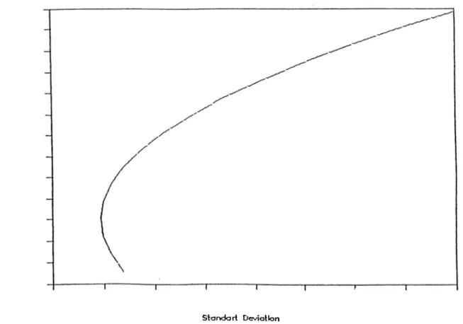
The shape of the efficient frontier is concave for the portion which is above the MVP, and convex for the portion which is below the MVP. The efficient frontier

E ffic ie n t Frontier

S ta n d a rt Dcviailon

Figure 3.1: Efficient Frontier

can not be convex. This is because combinations of assets can not have more risk than the risk found on a straight line connecting those assets.

An efficient mean-variance combinations set is called as the efficient frontier. A typical efficient frontier is presented in Figure 3.1 .

The efficient frontier should be mean variance efficient when compared with other combinations. This can be explained in other words as, the efficient frontier has no higher mean of returns and no less variance for any combination of risk-return level for a given opportunity set.

The construction of an efficient frontier requires the development of average return and variance of return formulas adaptation to a more than one asset structure or to the portfolio structure. Below, return and variance formulations are presented for the n asset portfolio case.

1. P o rtfolio H etlirn :

1=1

Ri : Rate of return on the asset.

X ,· : Proportion to invest from the asset.

2. P ortfolio V ariance : (8) p X ,· cr i=lj=l : Portfolio variance .

: Proportion to invest on the asset .

: Covariance between the and assets returns.

(9)

The mean-variance portfolio selection method can be formulated to obtain efficient frontiers, for a given set of investment objectives as follows.

m in-A Rp -f cTp, A > 0 A : Risk preference coefficient.

Rp : Portfolio rate of return. (Tp : Portfolio variance.

This objective function can be written as ;

(10)

n n

m in-A (X ;.T .R .)-f (X ; X i X j a i j ) , A > 0

'■=1 1=1 j=l (11)

The constraint set for the Standart model includes :

U n ity c o n s tr a in t, which forces all the resources to be invested :

1=1

(12) 't h e r e q u ir e d r a te o f r e tu r n c o n s tra in t, which ensures that a required rate of return which is denoted by R p will be earned by the constructed portfolio.

'y j XiRi — Rd (13)

t = l

t i p p e r a n d L ow er B o u lid s c o n stra ilit, which allows the investor to determine the combination and proportion of the investment from a given set.

, Li < Xi < Uiy {i = l,2 ,...,n ) (14) This m athem atical programming problem can be solved by using the quadratic programming techniques. The Application of the quadratic programming structure implicitly brings the Kuhn-Tucker conditions of the classical optimization theory, with one or more inequality constraints.

The Kuhn-'Tucker conditions for a two variable model can be w ritten as.

m i n max f(^X\, X2') (15) Subject to ; g{xi,X2) > 0 i l _ _ _ n V 6xi ¿ Ij ’ ■^?(a:i,a;2) = 0 j( x i,i2 ) > 0 A > 0 (16) (17) (18) (19) (20) The usage of Kuhn-'IUcker conditions, for one or more inequality constraint, will ehsure that, if the optimum can be found theU all a;,-’s will be positive [14].

For the solution of quadratic programming problems, several software packages are available both for the mainframes and PCs. On mainframfes Minos and on PCs Gams-Minos, Ginos, Hyper/Lindo can be given as well known examples.

In this study for the solution of the mean-variance portfolio selection problem Hy- per/Lindo - 1987 version is used. Certain changes are made in the modelling in order to make the model acceptable by the software package [22].

The preparation of the model to be solved is done with a m atrix generator. The m atrix generator created models according to the changing lambda values in MPS ( hiathem atical Programming Structure ) and these models are imported and solved for obtaining efficient portfolios and efficient frontiers.

3.1.3

single Index Model :

The Single index model is a simplified model for the portfolio selection problem. This model relays on a market index whicli measures the fluctuations in the market and its effects on the individual security returns. Market fluctuations’ effects are measured by the B eta ( ) coefficent.

The Single index model or the diagonal model is defined by Sharpe as follows [30] :

I = -^n+l + Cn+I Ei = Ai -f ) v:· = {Bl){Q nu + g .) c = (B ,)(B d(g„+i) (21) (22) (23) (24) (25)

B^ : Rate of return on the asset.

Ai : A constant return term which is independent of the market fluctuations. Bi : The beta coefficient.

/,· : The market index.

Ci : The error term.

Bi : Expected return of the asset.

1. P ortfolio R etu rn :

B p — ¿ ^ i B i — ¿ r ; ( j 4 , · - f B i l + C i ) t = l t = l

(26)

Ep : Portfolio ra te of retu rn . 2. P ortfolio V ariance t i = l j = l i = l or , (27) 1=1 1 = 1 7=1 1=1 cTp ; Portfolio Variance.

Cm '■ Variance of the market index.

a l: : Standart error of the estimator.

(28)

3. P ortfolio B eta t

As individual securities have beta coefficients, constructed portfolios have beta coefficients as well. Portfolio beta will me8isure the percent change in the port­ folio’s return when there is a one percent change in the fnarket index.

Bp = Y^XiBi

1=1

(29)

Bp : Portfolio beta .

4. Portfolio Alpha :

Portfolio alpha measures the fate of portfolio return whicli is independent of the market fluctuations that a portfolio can gain.

A.p — y \ Xi^i

1=1

(30)

Aj, ; Portfolio a lp h a .

In this study the Single index model is applied together with the Excess Return to Beta algorithm presented by Elton-Gruber and Padberg [12].

T ile E xcess R eturti to B eta algorithm :

The excess return to beta algorithm provides considerable computational conve­ niences for the portfolio selection problem under the index model [12] .

The objective of the excess return to beta algorithm can be summarized as finding a set that would maximize the objective of ;

^ _ (Rp R j) (31) p 4· = E"=, L U + i;r .i : Portfolio Variance.

; Variance of the market index. : Standart error of the estimator.

(32)

To find the optimal set that would maximize the derivative of <j> is taken with respect to each i,· and set equal to zero.

The optimal allocation will be performed according to excess return to beta formula :

z,· =

-C,l

A· ₍₃₃₎

1 -4- n-2 V" fL·

The proportion to invest from the security is calculated according to equation ( 34 ) which is presented below.

^0 __ Zi

U=i k .| (34)

The Xi values that will be obtained from the algorithm will ensure the constraint portfolio to be an optimal portfolio for a standart model.

Tills model presented by the equations ( 32 ) , ( 33 ) ,( 34 ) allows short selling of any security that is taken into analysis. However, if equation ( 33 ) is modified with equations ( 35 ) and ( 36 ) , then the Excess R eturn to Beta algorithm can handle models with no short sales. Basically, this modification is the inclusion of

the Kuhn-Tucker conditions to the optimization problem.

<l>k = (36)

Equation ( 35 ) uses set k as the set of stocks to be selected. And the inclusion rule for the algorithm is determined by the /x; , in equation ( 36 ) .

The inclusion rule for the algorithm is; select i as long as /x,· > 0.

Zi A Hi — IZf

A — + /t.· (36)

The proportions to be invested according to the excess return to beta algorithm can be calculated according to the equation ( 34 ) again. However, the absolute value operator in the denominator becomes redundant, since short selling is not allowed.

3.2 Assumptions of the Study :

The assumptions behind the mean-variance model and single index model are im­ portant for the evaluation of this study’s findings and potential real life applications.

In both of the models applied, the investors are assumed to be rational, who prefer more to less and assumed to be risk averse. Also all of the relevant information should be quantifiable by the investors. xVlsq, in both models all of the funds were forced to be invested and no short sales are allowed.

3.2.1

Mean - Variance Model :

In this study, for the Markowitz model, a single period, utility maximizing strategy is used together with the usage of ex post data.

The single period utility maximization restricts the portfolio selection process as a one period act, which should, infact be a continous process of reviewing and reallo­ cating. Also the usage of ei post data is another im portant point to be considered

when interpreting the findings of this study.

3.2.2

Sitigle Index Model :

Single index model totally depends on the index model selected and used. Therefore the calculations with different indexes will possibly present different results. There are certain assumptions of the single ihdex model, these are:

1. E{ei) = 0 , Vi

The mean of error terms should be normally distributed.

2. E(ei(Rm — = 0 , Vi

Index should be unrelated to unique return for the securities analyzed.

3. E {ei,ej) = 0 , V i,j

Securities should only be related through a common response to market. Er­ ror terms should not be correlated.

4

. E{ei,eiY = cli

By definition variance of e; is (7^,· which is a constant.

r i

5. E {ei{R ^ - Rm)Y = al

By definition variance of Rm is cr^

4. DATA :

The d ata used for this study is obtained from the Istanbul Securities Exchange publications. Weekly closing prices are used for the calculation of capital gains on stocks. The stock split and capital increase data is obtained from the thé Capital Markets Board publications , and used for thé modification of the closing prices for the correct calculation of capital gains. This modification is presented in this section , in equation ( 1) .

The time series used for this study covers 102 weekly observations from January 1986 to December 1987.

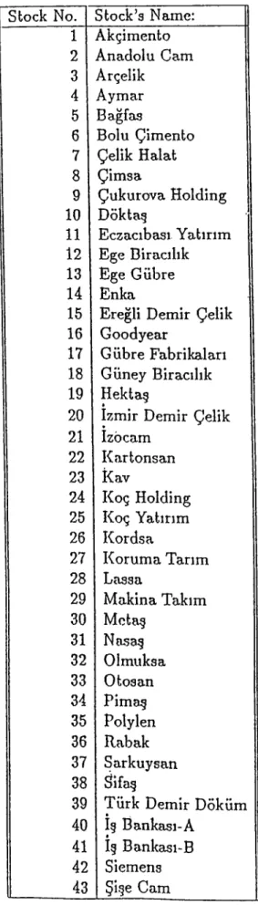
The stocks analyzed are selected from the first market of the Istanbul Securities exchange. For consistency, a set of 43 stocks are taken throughout this period. Company names are presented in Table 4 .

The classification that was used in the Istanbul Securities Exchange required cer­ tain modifications to be made for obtaining correct capital gains figures on the

price data. As the corporations announce capital increases and issue stock splits,

four types of quotations are made in the market till the end of the capital increase period according to their right contents.

These quotation types are;

1. Old,

2. Preemptive rights on , 3. Stock split right on ,

4. New .

The rate of return at the end of the capital increase period should be corrected according to the following equation .

r; = ( P . + I - ( P „ r / m ) )

r,· : Rate of return on the period.

P{ : Price of old quotation on the period.

P,ar ■ Price of the stock split right on quotation,

m : number of shares to be received as the result of the stock split.

(

1

)

If sucli a modification is not performed, then because of the enourmous price changes at the end of the capital increase periods, superflorous negative rate of returns can be observed.

For the single index model, the beta coefficients are estimated by using linear re­ gression technique, with the functional structure of the equation ( 21 ) in section 3.1.3.

Stock No. Stock’s Name: i Akçimento 2 Anadolu Cam 3 Arçelik 4 Aymar 5 Bağfas 6 Bolu Çimento 7 Çelik Bialat 8 Çimsa 9 Çukurova Holding 10 Döktaş 11 Eczacıbası Yatırım 12 Ege Biracılık 13 Ege Gübre 14 Enka

15 Ereğli Demir Çelik

16 Goodyear

17 Gübre Fabrikaları 18 Güney Biracılık

19 Hektaş

20 İzmir Demir Çelik

21 Izbcam 22 Kartonsan 23 Kav 24 Koç Holding 25 Koç Yatırım 26 Kordsa 27 Koruma Tarım 28 Lassa 29 Makina Takım 30 Metaş 31 Nosaş 32 Olmuksa 33 0 tos an 34 Pima§ 35 Polylen 36 Rabak 37 Sarkuysan 38 ¿ifaş 39 Türk Demir Döküm 40 İş Bankası-A 41 İş Bankası-B 42 Siemens 43 Şişe Cam

Table 4.1: List of Stocks’ analyzed. 29

The coefRcients calculated for the IMKB index is presented below in Table 4.2. bhock K Id.No. Square 1 2 3 5 6 7 8 9 10 11 12 13 14 15 16 17 16 19 20 21 22 23 24 25 26 27 28 29 30 31 32 33 34 35 36 37 38 39 40 41 42 43 0.2559 0.0000 0.1579 0.0018 0.1293 0.0395 0.1461 0.1857 0.1213 0.1961 0.0032 0.0211 0.0777 0.0009 0.0004 0.1431 0.0458 0.0009 0.0735 0.0131 0.0797 0.0738 0.1444 0.1461 0.0955 0.3060 0.0218 0.3089 0.0263 0.0078 0.0048 0.1985 0.0380 0.0042 0.0031 0.0525 0.0922 0.2276 0.1734 0.0033 0.0000 0.0210 0.0581 F 27.858 0.002 16.316 0.087 14.116 1.894 16.594 18.703 13.389 20.007 0.271 1.622 5.979 0.031 0.033 6.346 3.749 0.055 5.001 0.875 7.279 7.512 12.154 13.685 9.512 41.446 2.165 40.678 1.455 0.355 0.411 19.320 3.401 0.059 0.068 5.323 9.753 6.484 20.150 0.171 0.000 1.655 5.485 B (1) 0.7127 -0.0157 0.6389 -0.0846 0.7604 0.3589 0.5925 0.6447 0.6393 0.7751 0.0904 0.2994 0.5362 0. 1122 -0.0487 0.9160 0.3540 0.0816 0.5649 -0.4057 0.5072 0.3860 0.5387 0.5261 0.5004 0.8231 0.2787 1.0448 -0.4686 0.3238 0.1834 0.9429 0.4306 -0.8786 -0.1758 0.3991 0.4768 ■· 1.4597 0.6726 0.0922 0.0010 0.1952 0.4887 B (0 ) h(B(D) 1(0 (0)) O.W. 0.0103 0.0567 0.0184 0.0387 0.0159 0.0222 0.0008 0.0205 0.0219 0.0104 0.0197 0.0204 0.0210 0.0454 0.0237 0.0296 0.0135 0.0330 -0.0013 0.0430 0.0189 0.0133 0.0156 0.0130 0.0167 0.0074 0.0232 0.0157 0.0473 0.0249 0.1664 0.0228 0.2553 -0.0039 0.0175 0.0168 -0.0175 0.0163 0.0328 0.0113 0.0188 0.0123 5.278 -0.044 4.039 -0.296 3.757 1.376 4.074 4.325 3.659 4.473 0.521 1.274 2.445 0.179 -0.183 2.519 1.936 0.234 2.236 -0.935 2.698 2.752 3.486 3.699 3.084 6.438 1.471 6.378 -1.207 0.595 0.641 4.395 1.844 -0.244 -0.261 2.307 3.123 2.546 4.489 0.413 0.005 1.287 2.342 0.892 1.840 1.361 1.586 0.920 0.998 0.070 1.604 1.463 0.701 1.323 1.010 1.119 0.850 1.043 0.957 0.865 1.106 -0.059 1.158 1.177 1.108 1.182 1.069 1.202 0.670 1.429 1.121 1.425 1.051 1.018 0.905 1.139 0.846 -0.069 1.175 1.284 -0.360 1.269 1.716 0.627 1.450 0.686 1.7092 2.6079 2.0312 2.1746 2.5350 1.2588 2.1633 1.7568 2.3625 1.6269 1.3339 1.5381 1.8025 1.7729 1.8880 2.2285 1.8562 1.5741 1.8558 1.8445 1.6911 2.3203 1.8355 1.9916 1.8758 I.9603 2.4065 1.9289 •1.2841 1.8879 1.4747 1.8832 1.7576 2.1734 1.5548 1.7848 1.9492 1.3861 2 .20-19 1.5682 1.8359 2.0066 1.7129

ral)le 4.2: Regression result.s for IMKD index Returns

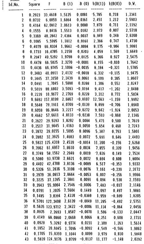
Beta, statistics calculated presents poor F and t test values for the IMKB index. Therefore, another index is developed as the weekly returns’ average. The coeffi­ cients calculated for the Return index is presented below in Table 4.3.

StcKk I d.No. 1 2 3 4 5 6 7 8 9 10 11 12 13 14 15 16 17 18 19 20 21 22 23 24 25 26 27 28 29 30 31 32 33 34 35 36 37 38 39 40 41 42 43 R Square 0.2923 0.0732 0.4164 0.1555 0.3369 0.1085 0.4079 0.1733 0.2947 0,4478 0.4436 0.3483 0.3445 0.0491 0,5019 0.2239 0.6692 0.5648 0.6059 0.4662 0.2627 0.2517 0.2872 0.2882 0.5822 0.3962 0.3748 0.5080 0.4402 0.5326 0.2979 0.3225 0.3943 0.0791 0.1485 0;5701 0.5635 0.0935 0.4149 0.0929 0.1852 0.1705 0.5839 F 33.4618 6.0059 62.0812 8.8416 48.2842 5.5995 66.8334 16.4785 40.5292 66.5025 66.9745 40.0911 37.3150 1.7045 88.6802 10.9677 157.8199 79.1911 96.8646 57.6611 29.9293 31.9645 29.0155 32.3925 125.4318 61.695? 58.1562 93.9738 42.4708 51.2836 36.0813 37.1395 55.9964 1.2035 3.8394 127.3408 123.9712 2.2693 68.0860 5.3292 20.6945 15.8359 124.9176 B (1) .8 (0) t(B(D) t(B(0)) D.W. 1.5135 1.6864 2.0613 1.5513 2.4384 1.1812 1.9662 - 1.2158 1.9798 2.3270 2.1098 2.4132 2.2439 1.5888 3.5093 2.2769 2.686? 4.0709 3.2217 4.8133 1.8292 1.4163 1.5095 1.4683 2.4539 1.8610 2.2948 2.6621 3.8136 5.3108 2.8664 2.3881 2.7546 7.5604 2.4228 2.6139 2.3422 1 .858? 2.0668 0.9774 1.7096 1.1044 3.0799 0.0081 0.0361 0.0080 0.0182 0.0037 0.0161 -0.0094 0.0203 0.0125 -0.0001 -0.0035 -0.0018 0.0061 0.0288 -0.0194 0.0228 -0.0107 -0.0139 -0.0272 -0.0238 0.0084 0.0050 0.0096 0.0072 -0.0014 0.0034 0.0019 0.0072 -0.0089 -0.0076 -0.0053 0.0091 -0.0006 0.1449 -0.0369 -0.0049 -0.0006 -0.0070 0.0066 0.0231 -0.0092 0.0099 -0.0137 5.785 2.451 7.879 2.973 6.949 2.366 8.175 4.059 6.366 8.155 8.184 6.332 6.109 I . 306 9.417 3.312 12.563 8.899 9.842 7.593 5.471 5.654 5.387 5.691 I I. 200 7.855 •7.626 9.694 6.517 7.161 6.00? 6.094 7.483 I . 097 I . 959 I I . 285 I I . 134 I . 506 8.'251 2.'309 4.549 3.979 I I . 177 0.718 1.212 0.711 0.807 0.248 0.747 -0.904 1.569 0.927 -0.010 -0.-321 -0.115 0.385 0.552 -1.202 0.772 -1.159 -0.706 -1.924 -0.868 0.580 0.460 0.793 0.646 -0.156 0 .'3'39 0.149 0.608 -0.353 -0 .2'39 -0.256 0.538 -0 .0-37 0 . 497 -0.699 -0.492 -0.064 -0.133 0.608 1. -263 -0.566 0.830 -1.148 1 . 2-341 2.5903 2.1192 2.5718 2.6200 1.4730 1.9981 1.6649 ■ 2.5475 1.7642 1.5785 1.9475 1.8607 2.0247 2.0488 1.5834 1.9992 1.8940 2.0053 2.1346 1.7619 2.7243 1.5801 2.4403 2.6268 1.9456 2.7524 1.8004 1.9332 2.3172 1.9966 2.1593 2.1146 1.9881 1.8205 2.5751 2.0456 2 .044? 2.1731 1.5614 1.9862 1.9848 2 .0-292

Table 4.3: Regression results for Return index Returns 31

5. FINDINGS OF THE STUDY AND

CONCLUSIONS :

5.1

Mean - Variance Model :

The calculated efficient frontier is presented for the Markowitz model, below in Fig­ ure 5.1 for Xi > 0 and i ; < 1 and a;; = 1 together with no short sales constraint.

E ffic ie n t F r o n tie r

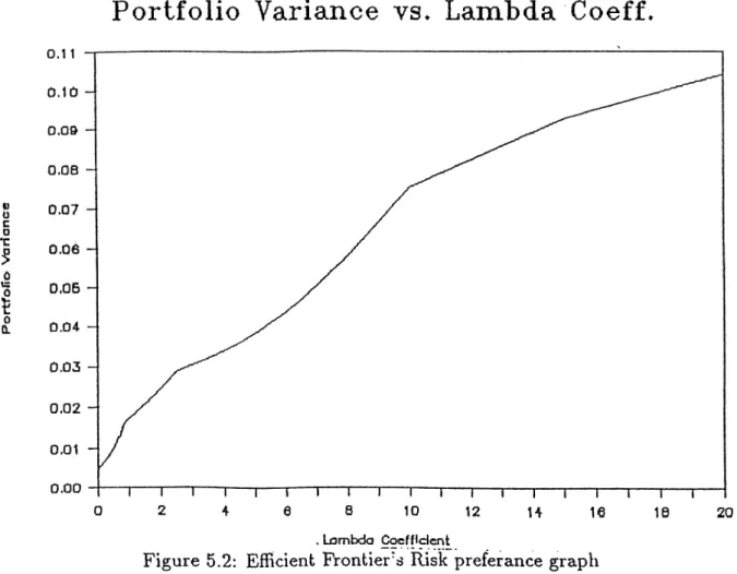
P o r tfo lio V ariance vs» Lambda C oeff.

, Lambda Coefficient

Figure 5.2: EfRcient Frontier'^ Risk preferance graph

The risk and return characteristics of the constructed efficient frontier together with the objective function value , iterations performed and number of variables in basic are presented in Table 5.1 . The characteristic properties of the constructed efficient frontier in Figure 5.1 for the A value , iteration number, basic variable set and the minimum variance portfolio allocation under the Markowitz model are presented in Figures 5.2, 5.3 , 5.4 and 5.5.

L am bda Coeff. vs. Ite r a tio n N u m b er

Lambda Coeffident

Figure 5.3: Efficient Frontier’s Iteration Summary graph

5.2

Single Index Model :

The calculated efficient frontier is presented in Figure 5.2 for the Single index model under the Excess return to beta algorithm.

’ortfolio R eturn Portfolio Variance lambda | Objective Function Value Iterations Ba^ic Variable Number 0.014614 0.020921 0.023381 0.024741 0.025747 0.026752 0.027526 0.028300 0.029097 0.029917 0.030673 0.031534 0.032361 0.032361 0.033578 0.034144 0.034661 0.034923 0.035119 0.036725 0.037817 0.038778 0.039030 0.039281 0.039533 0.039784 0.040035 0.040287 0.040538 0.040790 0.041041 0.041292 0.041544 0.041795 0.042047 0.042301 0.042519 0.043273 0.043600 0.043600 0.043600 0.043600 0.004793 0.005430 0.006037 0.006500 0.006952 0.007505 0.008008 0.008588 0.009265 0.010044 0.010837 0.011828 0.012862 0.012862 0.014565 0.015442 0.016288 0.016744 0.017105 0.020920 0.024741 0.029011 0.030395 0.032030 0.033916 0.036053 0.038442 0.041083 0.043974 0.047118 0.050512 0.054158 0.058055 0.062204 0.066604 0.071314 0.075571 0.092907 0.104146 0.104146 0.104146 0.104146 0.00 0.10 0.15 0.20 0.25 0.30 0.35 0.40 0.45 0.50 0.55 0.60 0.65 0.70 0.75 0.80 0.85 0.90 0.95 1.50 2.00 2.50 3.00 3.50 4.00 4.50 5.00 5.50 6.00 6.50 7.00 7.50 8.00 8.50 9.00 9.50

lo.do

15.00 20.00 30.00 40.00 50.00 0.002395 0.000621 0.000490 0.001700 0.002960 -0.004270 -0.005630 -0.007020 -0.008460 -0.009930 -0.011450 0.013000 -0.014600 -0.014600 0.017890 -0.019570 -0.021280 -0.023010 -0.024790 -0.044620 0.063260 -0.082430 -0.101890 -0.121470 -0.141170 -0.161000 -0.180950 -0.201030 -0.221240 -0.241570 -0.262030 -0.282610 -0.303320 -0.324160 -0.345120 -0.366200 -0.387410 -0.602630 -0.819920 -1.255920 -1.691920 -2.127920 17 20 20 22 20 19 19 19 18 17 17 17 16 16 15 15 14 12 12 9 9 8 8 8 8 8 8 8 8 8 8 8 8 8 8 7 7 6 5 3 3 3 11 14 12 12 12 11 11 11 12 13 13 13 12 12 11 11 10 8 8 5 5 4 4 4 4 4 4 4 4 4 4 4 4 4 4 3 3 2 1 1 1 1

Table 5.1: Markowitz model Efficient Frontier properties

No. of B a sic V ariables vs. Lam bda C oeff

Figure 5.4: Efficient Frontier’s Basic variable summary graph

M inim um V ariance P o rtfo lio

E ffic ie n t F ron tier for th e SIM

Figure 5.6: Efficient Frontier under the Single Index model

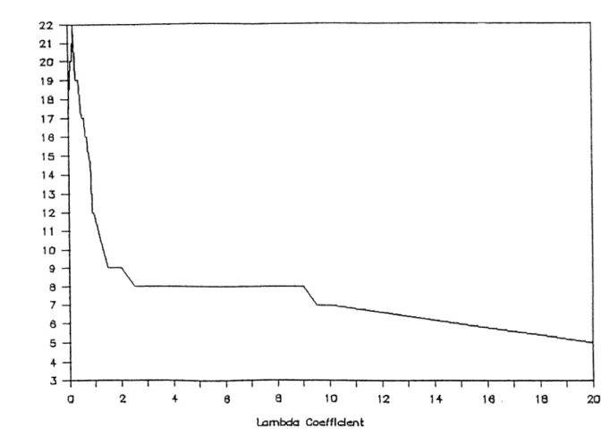
Portfolio beta and alpha are calculated for the single index model and presented below in Table 5.2 and in Figures 5.8, 5.7.

A value Portfolio Beta Portfolio Alpha 0.000 1.719 0.0087 0.001 1.726 0.0088 0.002 1.733 0.0089 0.004 1.760 0.0092 0.006 1.816 0.0093 0.008 1.856 0.0097 0.010 1.909 0.0101 0.015 2.017 0.0113 0.020 2.093 0.0128 0.025 2.244 0.0160 0.030 2.478 0.0218 0.035 3.083 0.0326 0.040 3.531 · 0.0441 0.045 4.455 0.0551 0.050 6.854 0.0901 0.055 7.283 0.1096 0.060 7.648 0.1343 0.065 7.799 0.1447

Table 5.2: Portfolio Alpna and Beta under the Single Index model

P o rtfo lio B eta v e r su s Lambda v a lu e s

Figure 5.7: SIM portfolio beta versus Lambda coefficient.

The minimum variance allocation (MVP) under the single index model is presented in Figure 5.9 .

P o r tfo lio Alpha v e r su s Lambda v a lu e s

Figure 5.8; SIM alpha and beta values compared.

MVP u n d er SIM

Figure 5.9: MVP combination under the SIM model

Tho construcicfl cfRcirnt fionUers me ploUccl below to present the bnsic diflcrenccs in their risk return characteristics.

Markoi^itz and SİM E ffic ie n t F ro n tiers

Return

Ö Markowllr -f Slnçle Index

Figure 5.10: SIM and MarkowiU EiTicicnt Frontiers comparison

The comparison of these two models according to the mean-variance criterion im­ plies that the investors should prefer the Markowitz efTicient frontier to the .single index model efficient frontier, because for a given level of return Markowitz model has a lower level of risk and for a given level of risk, has a higher level of return. This result is because of the index that is utilized in the single index model. How­ ever, with an appropriate index that will satisty the assumptions of the single index model the findings for the ipdex model will surely change, and approach to the markowitz model efficient set.

5.3 C o n clu sio n s :

In this study Markowitz and Single index portfolio selection models are applied to the Istanbul Securities Exchange market securities.

The Markowitz model and Single index model portfolios, because of their different structures and assumptions, constructed different portfolios and efficient frontiers.

5.3.1

Findings :

The findings of the both models are as expected from the theory. As the level of the return from the portfolio increased, the level of the portfolio risk increased as well. Also as the portfolios become more risk taking ( A | ) the number of securities decreased and the corner portfolio one is reached for the both models.

Markowitz Model Findings :

The Markowitz model accepted 14 securities as basic for the maximum and one security to basic for the minimum. Therefore a set out of the 43 securities are con- tiniously preffered to another set, or to the inefficient set. In Markowitz model some of the securities are never accepted to the basic set. Those securities are presented below ; 1. Bağfaş 2. Çelik Halat 3. Döktaş

4.

Eczacıba^ı Yatırım 5. Ege Biracılık 6. Ege Gübre 7. Gübre Fabrikaları 8. Güney Biracılık 9. Hektaş

10. İzmir Demir Çelik

11. îzocam 12. Koç Yatırım 13. Kordsa 14. Makina Takım 15. Metaş 16. Nasaş 17. Olmuksa 18. Rabak 19. Sarkuysan 20. İş Bankası - B 21. Şişe Cam

The ÎVİVP of the Markowitz model ( A = 0) , the following securities are taken into the basic ; 1. Anadolu Cam 2. Bolu Çimento 3. Goodyear 4. Kartonsan 5. Kav 6. Koç Holding 7. Pimaş 8. Polylen 9. Si faş 10. İş Bankası - A 11. Siemens

Through out the delineation process three securities are continiously taken into the basic. Those are ;

1. Anadolu Cam 2. Korum a Tarım

3. Pimaş

The upper right end of the efficient frontier is only made of one security. T hat is the security of the Anadolu Cam corporation; These results should be interpreted carefully because, Pimaş stocks are traded on a very short period of time, out of

the 102 periods.

Single In d ex M odel Findings t

The SlM findings are different then the Markowitz model findings because of the model’s nature. In SIM the MVP consists of 42 securities, however the MVP con­ sisted of 11 securities in the Markowitz model. The MVP combination for the SIM is presented in Figure 5.9 of this section. MVP of the SIM only eliminated the 35‘^ security, whicli belongs to the Polylen Corporation.

As the R j increased, the basic variables changed and for most cases the following securities are left in the basic of the Excess Return to Beta model;

1. Anadolu Cam 2. Goodyear

3. Metaş 4. Pimaş 5. Lassa

The upper right corner of the SIM efficient frontier includes only one security. T hat is the Pimaş cooperation’s security. As it was mentioned in the previous part, Pimaş stocks being in the basic is because of it’s transaction periods being very short and

this should be interpreted carefully.

The single index model coefficients /?; and a; that are calculated and used for the excess return to beta algorithm calculations, are not statistically significant for some of the securities. The ^,· and a,· coefficients are not statistically significant because of the returns’ not having a linear functional format which is used in equation ( 21 ) . In the scope of this study, /?,■ and a,· coefficients are used for the demonstration of the excess return to beta algorithm and no best functional format fiting study is performed.

Some of the coefficients being statistically insignificant can be a drawback for real 44

life users. Non linear functional formats should be tried for better functional form fitings. One other point to be mentioned for the single index model is that, the /?; and a; coefficients totally depend on the market index th at is Used.

Here, for the correct estimation of the beta coefficients some of the following rela­ tionships should also be checked:

1. Dividend payout , 2. Asset growth , 3. Leverage , 4. Liquidity , 5. Asset size , 6. Earning variability , 7. Accounting beta ,

These variables can be used to develop a Fundamental beta coefficient for a stock [3].

The single index model excess return to beta algorithm is a simple but powerfull tool for the portfolio analysis. Once the value of the equation ( 34 ) or ( 35 ) is calculated according to the assumptions used, in section 3.1.3 , then the calculation of proportions can be done very simply and quickly.

This application can either be done with an application specific software or with a spreadsheet software. As it is mentioned, once the program or spreadsheet is pre­ pared then the calculation of the optimal proportions will become very fast. The single index problem can also be solved as a Mathematical Programming problem by replacing the variance with beta coefficient and calculating the rate of return according to the single index formulations as presented in section 3.1.3 in equations ( 21 ) to ( 25 ) . Such a formulation can be found in Jacob’s and Faaland’s study [19] [15] .

The potential investors or users of such tools should always keep in mind that each method has its limiting assumptions. Also each method will be looking at the problem from certain point of view. Therefore the best approach to the portfolio selection process should be a combined and revised methodology that would also include the fundamental analysis and technical analysis as well. Since in the real applications one other problem will be estimation of an ex ante data set, a combined