Г39
MONETARY DYNAMICS ;
EVIDENCE FROM COINTEGRATION AND ERROR CORRECTION MODELING
THE CASE OF TURKEY
A Thesis
Submitted to the Department of Economics
and the Institute of Economics and Social Sciences of Bilkent University
In Partial Fulfillment of the Requirements for the Degree of
MASTER OF ARTS IN ECONOMICS
By
Huseyin KELEZOGLU March , 1992
-Qui.11’A 1^1
н ь
Ü
3
f l
Л ц ь
I certify that I have read the thesis and in my opinion it
is fully adequate, in scope and quality, as a thesis for the
I certify that I have read the thesis and in my opinion it
is fully adequate, in scope and quality, as a thesis for the
degree of Master of Arts in Economics.
Ass. Prof, limit Erol
I certify that I have read the thesis and in my opinion it
is fully adequate, in scope and quality, as a thesis for the
degree of Master of Arts in Economics.
/
Assi s t . Osman Zaim
ACKNOWLEDGEMENTS
I would very much like to thank Prof. Dr. Subidey Togan for
leading me to this study and for his recommendations and
encouragements during the preparation of the study. I am also
grateful to Prof. Dr. Carl Christ, Dr. Ahmet Ertugrul, Dr. Osman
Zaim, Ass. Prof, limit Erol, Dr. Erol Çakmak, Dr. Seyyid Mahmud,
Dr. Sönmez Atesoglu, Dr. Haluk Akdoğan for their many helpful
suggestions, recommendations and invaluable guidance.
I also wish to express my deepest appreciation to Erdem
Basci, Murat Yulek for the opportunity I had benefited from
their experience and knowledge, and for their invaluable
ABSTRACT
MONETARY DYNAMICS :
EVIDENCE FROM COINTEGRATION AND ERROR CORRECTION MODELING THE CASE OF TURKEY
Hüseyin Kelezoglu MA in Econonaics
Supervisor: Prof. Dr. Subidey Togan
March, 1992, 51 Pages
This paper addresses Lhe issue of Les-Ling Lhe cointegration
relationship for a conventional money demand function and
constructing an error correction model CECMD of it to analyze
both long-run and short run dynamics by using Turkish quarterly
data during the period 1977:1-1989:4. The assumption that all
the determinants of the long run money demand function are
endogenous allowed the construction of ECM in vector
autoregressive CVARD form. This became much helpful on the
examination of temporal causality characteristics of the long
run Turkish money demand function.
Keywords: Cointegration, Level of integration,
Stationarity, Error Correction Model, Vector Autoregressive
TABLE OF CONTENTS
ACKNOV/LEDGEMENTS
ABSTRACT
I . INTRODUCTI O N... ... 1-4
II. COINTEGRATION AND ERROR CORRECTION MODELING...5-18
AD CointegraLion : An Overview... 5-16
A. ID Testing for the Order of Integration... 9-lS A. 2D Testing for Cointegration... 12-15
BD Error Correction Modeling... 16-19
III. THEORETICAL AND EMPIRICAL STUDIES ON MONEY DEMAND
FUNCTIONS... 20-24
AD Theoretical Development of the Theory... 20-20
A. ID Monetarist Approach... 20-20
A. 1. ID Quantity Theory of Money... 20-21 A.1.2D Modern Quantity Theory of Money... 21-22
A. 2D Neo-keynessian Approach. ... 22-22
BD Empirical Studies on Money Demand Functions... 22-23 CD Studies on Turkish Money Demand... 23-24
IV. EMPIRICAL ANALYSIS... 25-43
AD Testing for the Order of Integration... ..28-29 BD Cointegration. Equations... 29-37 CD Error Correction Models... 38-43
V. CONCLUSION... 44-45
I. INTRODUCTION.
In recent years, the idea of using cointegration vectors in the
study of nonstationary economic time series has motivated
tests of long run equilibrium relationships suggested by
economic theory. The theory of cointegration mainly comes from
the work of Granger C1981D, Hendry and Richard C1892!), Granger
and Weiss C1983!), Engle and Granger C1987D, Stock C1987D,
Philips and Ouliaris C1988D, Johansen C1988J , Joharisen and
JuseliusC1990J among others.
The determination of the short run dynamics, on the other-
hand, stimulated research to the construction of error
correction models CECND. The developments in cointegration
theory further promoted the development of the ECM building
exercise, the reason being the fact that the information
obtained from the cointegration method reveals short run
dynamics.
The paper addresses the testing of the cointegration
relationship in the context of money demand and forming an
error-correction model for the Turkish case. The research on
money demand generally assumes that there exists a stable
relationship between real money balances and the * set of
explanatory variables that explain it. If such a stable
relationship does not exist, then the formulation of the money
demand function will be invalid. The aim in this paper is to
some combinations of real money balances, real income,
interest r a t e , expected inflation and expected inflation Cv/hich
will be explained 1 aterO. For this end, the two step»
Granger-Engle method is used. To incorporate the short run
dynairdcs into the model. Vector Autoregressive ECM C VAR ECMD is
employed, treating each of the variables in question as
endogenous. This is because all variables are potentially
endogenous, even the money supply if we think that Central Bank
has to respond to the market forces in effect by soirie
adjustments, especially in the long run.
The organization of the paper is as follows. The following
section discusses in some length the fundamentals about the
cointegration, and ECM. The next section reviews the studies of
the money demand function together with the special
characteristics of Turkish money market. The third section,
examines the testing of the cointegration relation in terms of
different monetary aggregates, real income, interest rates and
expected inflation. The VAR ECM formulation of the money demand
function is also included in this section. The results,
conclusions and the suggestions are contained in the section on
conclusion.
DATA; Quarterly Turkish data for the period 1977:1-1989:4
is employed. The analysis is considered in terms of three
consists of currency in circulation and commercial demand
deposits, M2 represents the broader one which is made up of Ml
plus commercial time deposits and certificates of deposits, M3
is the broadest definition here and in addition to M2 includes
also public demand and time deposits, and foreign currency
deposits^. The expected inflation figure is constructed
assuming that the expectations are generated naively, that is
the yearly inflation figure of S. I . S. at time t is expected to
occur also at time t+1. In fact, the empirical evidence, for
example, by Basel Cl990D supports that assumption.
The other variables are the real GNP Ccalculated as nominal
GNP deflated by the wholesale price index published by S. I . S. D
2
and net nominal interest rates . Following YulekC1990D,
expected loss CELD series, is also employed. The calculation of
EL series is performed in two steps as follows:
CID In the first step, the net return from holding money,
for example M2 is calculated separately as shown below.
R1xCDD+R2^CTD
CID RR2 = where RR2 represents the net
M2 T h e th re © m o n th ly a v e r a g e s o f t h e s e m o n e ta ry a g g r e g a t e s a r e tak en a n d v e i g h t e d b y the t h r e e m o n th ly a v e r a g e o f th e v h o l e s a l e p r ic e in d e x p u b li s h e d b y S . l . S . C a lc u la t e d a s th e th re© m on th ly a v e r a g e s o f th e maximum n o m in a l y i e l d o n d e p o s it s b a s e d on com p ou n d ed r a t e s o f th re © a n d s ix month d e p o s i t s . A v e ig h t e d a v e r a g e o f th e in t e r e s t r a t e o f f e r e d . b y 5 0 o r m ore b a n k s in the T u rk is h b a n k in g s y s t e m i s ta k e n a s th e r e l e v a n t in t e r e s t r a t e .
return from holding M2 and R1 and R2 are the maximum net yield
on commercial demand and time deposits respectively. CDD and CTD
represents the stock of commercial demand and time deposits,
respectively. In the calculation, the net nominal return from
holding demand deposits are assumed to be zero or negligible. In
this way, the net nominal return from holding Ml becomes zero.
The net return from holding M3 is proxied by the net return
on M2 assuming that the net returns of the two definitions of
money will not be significantly different.
C2I> The expected loss term is simply the minus of the
expected real interest rate on M2. It also rep»resents the
expected loss term of M3 definition of money. The calculation
for the expected real interest rate from holding M2 is done as
foilows:
C2D RR2^=
Cl+RR2Ct:)D
-1 where PCtD represents yearly
Cl+PCtDD
realized inflation at time t. As can be noted, the expectations
II. COINTEGRATION AND ERROR CORRECTION MODELING
AD Cointegration: An Overview
Recent advances in time series methodology have shown that
most economic time series are both mean and/'or covariance
3
nonstationary . There are two solutions to overcome this
problem, one is detrending and the other is differencing the
series until stationarity is achieved. However, these tv/o
methods to achieve stationarity led to a discussion between
economists. For example, Plosser and Schwert C1978D argue that
most economic models should be estimated between the changes of
the variables. They assert that if the process is in fact of
4
the difference stationary CDSPD type , the detrending procedure
3
A p r o c e s s Is c a l l e d m ean a n d c o v a r i a n c e s t a t i o n a r y i f th e f o l l o v i n g c o n d it io n s a r e s a t i s f i e d ;
<i>. ECx<t)D=/J
<ii). C ovC X<t), X<t+T>D= ^<T> fo r a l l t a n d T .
The v i o l a t i o n o f th e f i r s t c o n d it io n m akes th e s e r i e s m ean n o n s t a t i o n a r y . T h e s e c o n d c o n d it io n m e a n s that th e c o v a r i a n c e b e t v e e n t v o m em bers d e p e n d s o n ly on t h e ir d is t a n c e in tim e a n d the v i o l a t i o n o f th at c o n d it io n c a u s e s th e p r o c e s s to b e c o v a r i a n c e n o n s t a t io n a r y .
4 I f a tim e s e r i e s s h o w s a tre n d in th e m ean b u t n o t re n d in the v a r i a n c e , s u c h s e r i e s a r e c a l l e d b y N e l s o n a n d P l o s s e r (1PP2), “t re n d s t a t i o n a r y p r o c e s s e s <TSP)". A n e x a m p le a m odel i s th e f o llo w in g : y = a + bt + u ^ t t w h e re u^ i s a w h ite n o is e p r o c e s s . (c o n t in u e d in th e n ext p a g e ) o f su c h
v^ill resul'L in variances increasing over 'Linrie. This will result
in violation of the many of properties of the least squares
estimators and tests of significance. On the other hand, if
differencing is applied, then the result will be, even if the
process is of TSP type, at most inefficient estimates.
Therefore, Plosser and Schwert C1978D offered differencing the
series as a solution if nonstationarity problem is encountered.
However, Engle and Granger C1987D note that differencing
results in a loss of valuable lon^ run in/ornvat ion in the data,
and present the concept of cointo^;rat ion as a solution to the
nonstati onari ty probiem.
Engle and Granger C1987Z) claim that even though economic
time series may wander through time, econoiriic theory often
suggests that some set of variables cannot wander too far away
from each other, that is, they should obey certain equilibrium
constraints. Examples of such series may be wages and the price
level, prices of the same commodity in different markets, money
supply and prices, real interest rates in different countries
Cif capital is free to moveD. In this context, cointegration
means that although the individual time series are
On Ih© o th e r h an d, i f a iim © s e r i e s c a n b e m o d e le d a s y - y = + e
^ t ^ 1 - 1 t
v h e r© vs s t a t i o n a r y p r o c e s s v i t h m ean z e r o a n d c o n s ta n t v a r i a n c e , s u c h p r o c e s s e s a r e c a l l e d b y N e l s o n a n d P lo s s e r
nonstationary, one or more linear combinations of these
variables can be stationary. In this sense, a finding of
cointegration would imply that there is a stable long run link
between the time-series considered.
Consider, for instance, a pair of time series each
of which is ICID^. It can be argued that any linear combination
of these variables will in general be also ICID. The celebrated
result by Engle and Granger Cl987D, asserts that if there exists
a constant b such that
C3D e = X - by
i t i
v/here e is ICOD, and both x and y are ICID, then x and y will be
said to be cointegrated. The factor b is called the
cointegrating parameter. If there exist cointegration, b must
be unique in the bivariate case^. This is because another
factor Cb+aD generates an additional term C-ax^D, which is
nonstati onar y by definition. In model C3!), the series e^
represents short run deviations of the system from its long run
equilibrium. In this sense, it can be called &q'atlibrt'am
I I c a n b e sh ow n m a th e n n a tlc a lly th a t a tim e s e r i e s w h ic h i s n o n s t a t io n a r y in l e v e l s b u t s t a t i o n a r y a f t e r d tim es d i f f e r e n c i n g , h a s d n um ber o f u n it r o o t s . G r a n g e r a n d E n g le <1P87> h a v e p r o p o s e d a new ly p © o f c l a s s i f i c a t i o n , t h e y c a l l th e v a r i a b l e s th at a r e s t a t i o n a r y in l e v e l s a s " i n t e g r a t e d o f o r d e r z e r o ", d e n o te d a s KO>, th o s e th at b e c o m e s t a t i o n a r y a f t e r ta k in g f i r s t d i f f e r e n c e s . I d ) a n d t h o s e th a t b e c o m e s t a t i o n a r y a f t e r t a k in g s e c o n d d i f f e r e n c e s I<2) an d s o o n . <5 In c a s e w h e re t h e r e a r e m ore th a n tw o e c o n o m ic tim e s e r i e s w h ich a r e c o in t e g r a t e d , th e n t h is v e c t o r must n ot b e u n iq u e .
error . The stationarity of this error is a requirement for the
series to be cointegrated. Since by cointegration, it is
implied the two series and y^ cannot drift too much away from
each other in long run and if there occurs deviations in the
short run, they are forced to converge to their long run steady
state path by the economic forces such as market mechanism,
government or some others.
The cointegration between a vector of economic time series
also requires that the vector series are of the same order of
integration. This is because the variables which have different
orders of integration have different temporal p-»roperties
CGranger C1987DD and neglecting that fact results in spurious
regression problem.
One may ask what happens when the economic time series are
not of DSP type but rather of TSP type. That is, the model with
no trend in the variance but only a trend in the mean. Granger
C198GD, as an answer to that question, asserts that for such
vector of time series to be cointegrated in a meaningful sense,
the trend should be the same kind of functions of time.
Consider, For example.
C4:> X = f CtD + x ^ t X t T h e term e q u ilib r iu m i s u s e d in d i f f e r e n t m e a n in g s b y e c o n o m is t s . The term h e r e (c o n t in u e d in th e n e x t p a g e ) d e s c r i b e s th e t e n d e n c y o f th e e c o n o m ic s y s te m to a p p r o a c h to w a rd s a lo n g ru n e q u ilib r iu m , r a t h e r th an the b e h a v i o r o f th e e c o n o m ic a g e n t s .
C 5 D у = f C t D + y ; l X t w h e r e x ' , y ^ a r e I C I D t b u t o f t h e D S P t y p e . 1 e t C 6 D e = X - A y =f CtD - A f CtD + - Ay^. X у i t
Here, for to be ICOD, i . e. , x^and to be cointegrated, the
following two conditions must hold;
CiD e should have no trend in the mean, so that
i
C7:) f CtD = Af CtD for all t.
X у
CiiD x^ , y^ should be cointegrated with the same value
of A as the cointegrating parameter.
Mow, having examined the time series properties and
reviewed literature on cointegration, we are ready to discuss
how to test for cointegration. However, since the theory of
cointegration requires the series to be of the same order of
integration, it is better to first discuss the issue of testing
for the order of integration.
A. ID Testing For the Order of Integration:
Since most economic time series are found to be ICID, it is
most appropriate to discuss how to test whether a time series is
of ICID against the alternative that it is stationary. However,
ICID processes, as we have already discussed, can be classified
coi nlegr ati on changes depending on v^hether the series in
question is of DSP or TSP type. If the series is of DSP type,
then that means that the nonstationarity is due to stochastic
trends and differencing is the appropriate method to achieve
stationari ty. If the series is of TSP type, then the
nonstationarity is best represented by a deterministic time
trend and the appropriate method is to estimate regression on
time and utilize the residuals from that regression as the
detrended series. So, we have to test first, the hypothesis that
the series has a unit root against the alternative that it does
not and second, the hypothesis that the nonstationarity is due
to a stochastic time trend against the alternative that the
nonstationari ty is due to a deterministic time trend. To
test these two hypotheses, a test, which is called Augmented
Dickey Fuller CADF3) test, is developed by Dickey and
FullerC1981D and consists of estimating the following model by
Ordinary Least Squares COLSD
C8D Ax = a + C p “l D X + 6t + .E XjAx . + e
t ^ l - l t
where e^ is white noise, A is the difference operator, Ax^is the
first difference of the variable being tested, t is the time
trend and p is the first order autocorrelation coefficient, 6 is
the coefficient of the time trend, and X / s are the coefficients J
of the lagged differenced terms. The terms Ax^ ., j=l,2,...,k,
represent autoregressive approximations of the moving average
maximum lag k is carried out by examining the autocor r el ati on
and partial autocorrelation function of the first difference of
variables. The maximum lag reported is determined by the last
statistically significant Ca conventional t-statistic is usedD
lag after allowing k to vary from one to the highest possible
lag following Ahking C1990D. The process is assumed to have a
constant or drift. The process has a unit root if p=l > i . e. ,
Cp-1D=0 and the null hypothesis of unit root is rejected if it
is found statistically that C p-ID^. However ^ the test
statistic for this procedure is not the usual student^s t
distribution but rather is the one tabulated in Fuller C19 7 6 D ,
table 8.5.2. For the second hypothesis, the series is said to
be of DSP class if Cp-1D=0, 6=0 and the TSP class if the
null hypothesis is rejected, i . e. , if Cp-lZ)^, 6 ^ . This test
is in fact a likelihood ratio test and the test statistics are
computed as the standard F-test. The critical values are given
in Dickey and Fuller Cl981D, table VI.
The rejection of the second hypothesis suggests the
presence of a deterministic time trend. The appropriate method
in this case is first to regress the time series against a
constant a time trend, that is detrending, and get the residuals
from this regression as the detrended time series CAhking,
1990D. The next step is to perform the ADF test for unit root
by estimating the following regression by OLS;
c q:> e = a + pe + Z XjAe + u
t ^ t - l = 1 ^^ i - j i
Vv'here is the detrended time series and is a white noise
process. The null hypothesis in this case is p=l , that is e^ is
a unit root process against the alternative that it is not.
Here again> the test statistic is not the usual student ^s
t-distribution but the one that is reported in Fuller C 1 9 7 6 D ,
table 8.5.2. In this way, we first isolated the deterministic
time trend from the series and then sought for whether the
series in question is a unit root process or not.
A. 2D Testing for Cointegration:
To test for cointegration between a pair of time series,
that are found to be ICID, Engle and Granger C1987D, suggests
forming the following cointo^ratin^ r^^r&ssion;
CIOD X = a + fty + e
t ^ t i
and then estimate this equation by ordinary least squares C O L S D ,
and further test if the residual series, e^are stationary or
not. If the residuals are stationary, then the cointegrating
vector is Cl ,-a ,-/? D. Here, a represents the coefficient of
the constant term and about the presence of the constant term,
Johansen and Juselius C1990D argue that if the examination of
the data reveals that the series exhibit linear trends, then the
above cointegrating regression should be run with a constant
stock Cl 9871) has shown that OLS estimates of the
2 —2
cointegrating vector are highly efficient with variances a
v/hereas in the normal situation they are o' XT , T being the
sample size. Stock further shows that the estimates are
2 —1
consistent with an o* XT bias. In sum, when the variables are
cointegrated, the estimates of the cointegrating regression will
be far more precise than with I COD variables, and this result is
known as sxip&r consts te^ncy.
Testing of the residuals coming from the cointegrating
regression is in fact a unit root test and so, one can easily
apply the standard unit root tests, Dickey Fuller CDFD and
Augmented Dickey Fuller CADFD. ADF test have been already
examined in equation C8D. DF test is simply the estimation of
equation C8D by OLS without lagged difference terms. Again, our
interest from estimating that equation is the t-statistic
associated with the lagged level term. The critical values are
given in Hall C1986D for two and three variable cases. The null
hypothesis is again the same one claiming that Cp-1D=0 against
the alternative that Cp-ID^. The non-rejection of that
hypothesis implies that the series are not cointegrated, and the
rejection of it implies that the series are cointegrated. The
finding of cointegration would imply that although the series
themselves are nonstationary, their linear combination, that is
the residuals from the cointegrating regression, are stationary.
Other than the ADF and DF tests, one can also apply a test
called Cointegrating Regression Durbin V/atson CCRDWD to test for
cointegration. This stems from the fact that^ as noted by both
Hendry C1986D, and Granger C1986D , the Durbin V/atson CDVD
statistic of the residuals of the cointegrating regression
should not be too low otherwise, the series will be ICID. So,
Granger and Engle Cl9872), developed CRDV/ , which is simply the
DW statistic from the cointegrating regression. However, the
critical values are different from the ones in the usual DV/
tables and are tabulated in Engle and Granger Cl 9871) for two
variable case in tables II and III and in Hall Cl9862) for three
variable case. However, we do not use the ones reported in
Engle and Granger C19872) for they are only reported for two
variable cointegration regression. Since cointegration is
searched among more than two series, it is better to use the
critical values in Hall C1986D which are reported for three
variable case. For the four variable cointegrating regressions,
the distributions of the statistics is approximated by that of
the three variable case. Again, our null hypothesis is that
there does not exist a stable linear relationship between the
variables against the alternative that there does.
It is quite possible that more than a pair of series can
also be cointegrated. The problem with this case, however is
that more than one stable linear combination may exist. If such
a case occurs,the procedure developed by Engle and Granger
C1987D has a limiting use since it cannot detect the existence
of more than one stable linear combination. Johansen Cl9882) and
to detect the presence of more than one cointegration vector
Csee for the Johansen approach as well as other approaches
Dickey, Jansen, Thornton C1991DD.
One other problem with Engl e-Granger two step approach is
that it requires the researcher to choose one of the endogenous
variables and to put it on the left hand side as the dependent
variable. But, this brings the issue of nonuniqueness of the
cointegrating vector since the use of different left hand side
conditioning variables may yield a different cointegrating
vector. To overcome this problem using Engle-Granger two step
estimation procedure. Hall C1986!) argued that it is best to
examine all possible cointegrating regressions and choose the
one with the highest adjusted coefficient of determination as
the cointegrating vector. Hall C19S6Z) addresses this problem and
quoting from Stocks^ Cl985!) theorem 3 which establishes that the
cointegrating regression is consistent but subject to a finite
sample bias, argues that this bias seems to be related to the
overall goodness of fit of the regression, and so one may choose
the cointegrating vector as the cointegrating regression with 2
the highest adjusted R since it should be subject to the
smallest bias. Such a guidance is also provided in Hendry
2
C1986D saying that the bias will depend on R and in the case
where it is very near to one the cointegrating vector will be
approximately the same in all cases.
BD Error Correction Modeling CECMD:
ECM is a method of dynamic modeling developed mainly by
British econometricians. This type of model was first
#
introduced by Sargan C1964D and has been improved by David
Hendry and some other econometricians. The later development
mainly comes from the work of Davidson, Hendry, Srba and Yeo
C1978D, Davidson and Hendry C1981D, Hendry and Richard C1983!) ,
Hendry C1983D, C1986D. Recently, Engle and Granger C1987D
developed the model further by emphasizing the strong relation
between cointegration and ECM and argued that there exists an
ECM representation of cointegrated variables.
The basic premise of ECM is that people act to correct
their errors in the past. This approach implies that the
equilibrium relationships suggested by economic theory holds
only in the long run. Such equilibrium posited by economic
theory is by no means achieved in every period. There may be
some divergences from the equilibrium, i . e. , e^c^ui I ibrium e^rror
and people act to correct these errors in later periods by some
adjustment. Stemming from this idea, ECM relates the changes in
the cointegrated variables to lagged changes of the endogenous
variable itself and of other exogenous variables in the system,
and lagged EC term C^quilibrium error from the cointegrating
regression!). In this way, the change in the conditioning
variable in the cointegrating regression will be such that it
previous period, that is its response v/ill be in the way to
correct the short-run deviation of the system from its long -run
path. In this way, economy is pushed to the equilibrium
whenever it moves away from equilibrium. The advantage of ECM
combined with cointegration is that in this way, we incorporate
both short run and long run dynamics into one equation.
Furthermore, there does not exist any spurious regression
0
problem since all the variables are I COD.
To illustrate, suppose that we found cointegration
between and y^ in equation C 3D. To construct an error
correction model, we run the following regression by OLS;
CllD Ax = a + Z Ax
i l=1 i- L
p
Z 6l Ay
j=i t-J t - 1 w
where w is a white noise, e is the lagged error term from
the cointegrating regression.
The lag lengths k and p are determined by following
Hendry^s C1986D general to spoci ficc approach^ which involves
eliminating lags with insignificant coefficients.
The ECM formulation in Engle and Granger C1987D consists of
one equation as described above. In this paper, however,
following Miller C1991D, ECM model contains four equations for
8 S p u r i o u s r e g r e s s i o r » p r o b le m m ay e x is t i f f o r e x a m p le som e v a r i a b l e s a r e K O ) v h i l e o t h e r s a r e K l ) or som e o t h e r o r d e r o f in t e g r a t e d . T h e p r o b le m i s that th e te m p o ra l c h a r a c t e r i s t i c s o f t h e s e s e r i e s a r e d i f f e r e n t . S p u r io u s r e g r e s s i o n i s p a r t i c u l a r l y l i k e l y w h en th e c o e f f i c i e n t o f d e t e r m in a t io n e x c e e d s the DW s t a t i s t i c <see P l o s s e r an d S c h v e r t <1P78>). 17
Ml definition of real balances, and three equations for M2 and
M3 definitions of real balances. The first differences of the
logs of real monetary aggregates Ml, M2, M3, and of all other
variables are each functions of distributed lags of first
p
differences of themselves as well as lagged EC term . This kind
of ECM formulation in fact can be described as vector
autoregressive CVARD system constrained by the EC term. Such a
specification of the ECM implies that each variable acts as
endogenous. Furthermore, such a model building exercise
provides some interesting temporal causality interpretations
Csee Miller C1991DD. Cointegrated variables must reveal
temporal causality in at least one direction in the bivariate
case. Next, this temporal causality can exhibit itself in two
different ways. One can be understood by the standard Granger
causality test regressing the first difference of a variable on
the lagged first differences of itself and other possible
Cran^^r-ccLxistn^^ variables. The other can be understood by
M o re th a n o n e Lag o f th e e r r o r c o r r e c t io n term i s u n n e c e s s a r y . T h is i s b e c a u s e th e e f f e c t s o f th e l a g g e d e r r o r c o r r e c t io n term s a r e a l r e a d y in c lu d e d in th e r e g r e s s i o n b y in c o r p o r a t in g th e l a g g e d c h a n g e s o f th e a l l v a r i a b l e s <see E n g le an d G r a n g e r <1P87>>, A v a r i a b l e y ^ i s s a i d to b e G r a n g e r - c a u s e d b y a v a r i a b l e y ^ i f th e in fo r m a t io n in p a s t an d p r e s e n t y ^ h e l p s to im p r o v e the f o r e c a s t s o f th e v a r i a b l e y ^ . To e x p r e s s it d i f f e r e n t l y , a v a r i a b l e y^ i s G r a n g e r - c a u s e d b y th e v a r i a b l e y ^ i f it can b e p re d ic t e d m ore e f f i c i e n t l y v h e n th e in fo r m a t io n in p a s t a n d p r e s e n t y i s ta k e n in to a c c o u n t in a d d it io n to a l l o th e r 2 in fo rm a tio n in th e u n i v e r s e . L e t u s fo r m a liz e t h is c o n c e p t. A ssu m e O c o n t a in s a l l th e (c o n t in u e d in th e n ext p a g e )
regressing "the first difference of a variable on EC term- The
Granger test ignores the second channel and so may overlook
existing causality. So> inserting the libri'um error into
the VAR system as an exogenous variable allows the second
channel to be considered. r©l©va.nt 2v n fo r m a lio n d e fin e O' C y IOZ> I t ^ ' a v c iila b l© to a g © n ts up to p e r i o d o p tim a l f o r e c a s t It v a r i a b l e . i s s a i d to b e G r a n g e r - c a u s e d b y som e t v a r i a b l e y 2 a n d th e a s th e c o n d it io n a l m ean s q u a r e d e r r o r o f c o n d it io n a l on th e in fo r m a t io n in Q . T h e i f f o r <y^Cy 1 11 '|0 D < O' C y^ 1Q sI t ‘ t 2 8 |s<OD v h e r e O S t 2 6 |s<0 r e p r e s e n t s a l l th e i s not a v a i l a b l e in 2 s 1 S < t ! ) (J u d g e e l a l <1P85>. 19 in fo r m a t io n in o v h ic h
III. THEORETICAL AND EMPIRICAL STUDIES ON MONEY DEMAND FUNCTIONS.
ADThepretical Development of the Theory:
This section gives some important developments in the
theory of money demand. The theories on money demand can be
broadly put into two categories. The first one is the
Monetarist approach and the second one is the Neo-Keynessian
approach. In what follows, we highlight the basic elements of
the tv/o approaches to the money demand.
A. ID Monetarist Approach:
A. I.ID Quantity Thieory of Money CQTMD: This approach
takes the velocity of money and real income as constant and
stems mainly from the classic argument that there is a one to
one relationship between the money supply and the price level,
that is, the principle of neutrality of money. The classical
theory can be described by the following equation
C12D MV=PY
where M represents the money supply, V is the velocity of
circulation of money Caverage duration of holding cash
Equation 12 can be inverted so that one obtains
Cl 3D M=kPY
where k = 1 / V and as easily seen from the equation, the
premise of the QTM is that since k and Y are constant, an
increase in the money supply will increase only the price level.
A.1.2D Modern Quantity Theory CMQTD :
MQT is developed by Friedman C1956D. The comparison of QTM
and MQT will reveal the fact that they are basically the same.
However, Friedman, as different from QTM, takes the velocity of
circulation as a function of some variables and argues that the
money demand should be a function of the permanent income.
According to Friedman, permanent income is the return on a
widely defined stock of nominal wealth. This wealth consists of
money, bonds, equities, physical goods, human capital Csee for a
good review of the literature, Felderer and Homburg C1987DD. Now,
the Friedmanns money demand function may introduced as follows
C14D M. VCY, r, , r , CP/PD D = P. Y
b e
where r . r , and CP/PD are the rates of return on bonds,
b e
équités and expected inflation respectively.
A. 2D hJeo-Keynessian Approach :
On the neo-keynessi an approach, only liqxLidity pro/^re^nce?
¿h.eory CLPTD will be cited. LPT is developed by Keynes and can
be represented by the following equation
C15D M = LC Y , i D . P
where Y is the real income, i is the nominal interest rates on
alternative assets Cbonds and equities^, and P is the price
level. According to Keynes, demand for money arises because of
three sources. They are aD transactions demand for money which
is positively related to real income, Y. bD Precautionary
demand for money which is again positively related to Y. cD
Speculative deiriand for money which is negatively related to the
interest rates on alternative assets.
BD Empirical Studies on Money Demand Functions:
The demand for money, for long years, was one of the least
controversial topics in economics. However, the empirical
studies in 1970^s showed that the demand for money was unstable
in western countries and in U. S. A. For example, Enzler, Johnson
and Paul us in 1976 pointed out that the money demand functions
constructed with the data for the years before 1973 consistently
empirical literature on money demand functions the work of
Yoshida C1990DD. This motivated much work on the empirical
literature to improve the model specification. For that end,
new explanatory variables such as wealth and bank debits, or
dummy variables are added, or some other nriodel s are developed^^.
But even these did not help much to solve the unstability issue
of the money demand function.
Finally, EC modeling approach is proposed as a solution to
the unstability problem in the demand function for money. The
works of Hendry C1979Z), Rose Cl 985D , Joshida C1990D, Hendry and
Ericson C1991D among others have shown that the unstability
problem is resolved when the money demand function is formulated
as of ECM type.
CD Studies on Turkish Money Demand
The studies of Turkish money demand generally assumes a
partial adjustment model or a conventional model. Since Turkey
is a developing country, the inclusion of the expected inflation
rate generally gives a better fit. As noted by Gordon C1984D,
in an economy with very high inflation rates, inflation becomes
one of the major determinants of opportunity cost of holding
money. The work by Keyder C1988D, also supports this assertion.
11
The TT>odels s p e c i f i e d g e n e r a l l y a d a p t i v e e x p e c t a t io n s m o d e ls .
v e r e th e p a r t i a l a d ju stm en t
In Turkish money demand studies, it is generally found that
for the narrower definition of money, the relevant alternative
asset return is represented by the net nominal interest rate on
1 2
time deposits whereas for the broader definition of money, the
relevant opportunity cost of holding money is the rate of
inflation. The elasticity of the real income is generally found
to be near one. A recent paper by Yulek C1990D applies the
cointegration and error correction techniques to the estimation
of the velocity function and finds cointegration relation
between velocity of real Ml and M2, and real income.
12 A lth o u g h ^ the r a t e o f in t e r e s t in som e s t u d ie s i s fo u n d to b e i n s i g n i f i c a n t , t h is m a in ly stem s from th e s t r ic t r e g u l a t i o n o f th e g o v e r n m e n t o f th e in t e r e s t r a t e s b e f o r e li> 8 0 . A f t e r 1P80, l i b e r a l i z a t i o n p o l i c y in th e f i n a n c i a l s e c t o r in T u rk e y a l l o v e d in t e r e s t r a t e s to b e m ore f r e e l y d e te rm in e d b y the b a n k in g s e c t o r .
IV. EMPIRICAL ANALYSIS
MoneLary economists generally assume that the long run
money demand function depends in a stable way on a few number of
economic variables. These include the rate of return from
holding equities and bonds which can be represented by a mixed
interest rate, the real income, and especially in financially
developing countries on the inflation rate. The money demand
function is defined after the consideration of the combinations
of the real stock of wealth of an individual economic agent.
The stock of real wealth is assumed to composed off the
foilowi n g ;
CICD V^/P = Ml/P + TD/P + other real assets.
where Y/ZP is the stock of real wealth and Ml/P is the stock of
real Ml which includes the currency in circulation and demand 13 deposits and TD/P represents the stock of real time deposits
Other real assets represent the stocks of goods and estate w'hich
people owns.
For the precautionary and transactions motive, the real
income is well accepted as one of the functions of the money
demand. However, the determination of the opportunity cost of
13
H e r e , v e a ssu m e th at a l l th e f i n a n c i a l In v e s t m e n t s o f th e a g e n t s In th e e c o n o m y , v h e t h e r p u b lic o r p r i v a t e . Is I n c lu d e d In TD, th e sto c k o f r e a l tim e d e p o s it s .
holding money is not so easy. For that pur pose> the procedure
developed by WcCallum is utilized C1 989D . Consider ^ for examp^l e
that one tries to decide whether to hold all its real stock of
wealth in the form of Ml or in the form of alternative assets
such as TD and other real assets. For the return on Ml is very
small compar ed to the return on time deposits ^ we assume that
the net nominal return from holding Ml is zero or negligible,
then it is obvious that the real return from holding real Ml is
the negative anticipated inflation. There are two alternatives
against holding all stock of wealth in Ml, first one is TD and
the second is the goods and estate. Let the agent decide to
hold all its wealth in the form of TD. In this case, the
outcome of that decision as easily noted v/i 11 be the anticipated
real interest rate on M2. To calculate the opportunity cost of
holding Ml in this case, the return from holding Ml is simply
subtrac'ted from that of holding TD. Therefore, the opportunity
cost of holding Ml against holding M2 is the net nominal
interest rate on time deposits. Consider the case when the
individual agent decided to hold all its wealth in the form of
goods. Then, the real return of that decision v/i 11 be zero in
real terms. As a result, the opportunity cost of holding Ml
with respect to the alternative of buying and holding real
estate is minus the anticipated inflation rate. So, it can be
asserted that the relevant money demand function for Ml is;
C14D InCMl/'PD = a + /?lnY + XlnR + j^lnAP + e
where the logarithm of the real income, InR^is the
logarithm of the net nominal interest rate on T D s , and AP^ is
the anticipated yearly inflation rate. In the above
specification, since multiplicative effects assumed, all the
variables are in natural logs. This is the usual practice that
will be followed in the demand functions for real M2 and M3.
Coming to the specification of the demand function for real
M2 and M3, again with confidence one can say that the real
income is one of the determinants of the deiriand for them. Since
in equation Cl4D, the only alternative asset to holding M2 and
M3 is real estate, the real return from holding M2 and M3 should
be considered against the real return from holding real estate.
Let again the individual agent trying to decide how to allocate
his v^ealth between different kinds of assets decide to hold all
its v/ealth in the form of M2. Suppose that his decision involves
the real return from holding M2 and and that of real estate. It
is clear that the return from holding real estate is zero in
real terms. That implies the opportunity cost of holding M2
definition of money is real return on M2. Since real return on
M2 is the own return from holding M2, it is expected to be
positively related to the demand for it. As explained before,
the minus of the real return on M2 is termed as EL. The idea is
that if the agent anticipates a negative real return, it is also
EL from that decision. A consideration of these make the
following model appropriate for M2 and M3 definition of money;
C5D InCMi/Pj = a + /?lnY + XEL· + e
i ^ i t t i= 2,3.
The use of natural logarithms for variables apart from EL term
is for multiplicative effects are assumed to exist between the
variables in the model.
Having specified the money demand function, we. are ready to
seek for cointegration relation and error correction modeling
for the above functions. This involves three steps. The first
step is the determination of the orders of integration for the
variables that we use. Secondly, we estimate the cointegration
regressions by OLS, using the variables which are found to be
ICID and later test the cointegration relation by using CRDW, DF
and ADF statistics. Lastly, The VAR-EC modeling is studied.
AD Testing the Order of Integration
As we have already mentioned, firstly the hypothesis that
the series has a unit root against the alternative that it does
not and secondly, the hypothesis that the nonstationarity is due
to a stochastic time trend against the alternative that the
nonstati onar ity is due to a deterministic time trend will be
tested. To test these two hypothesis, ADF and likelihood ratio
tests will be utilized. The reported results in table I are
derived from the estimation of equation C8D. The maximum lag
conventional t-statistic is usedD lag after allov/ing k to vary
from one to the highest possible lag.
The examination of table I Vv^i 11 reveal the fact that most
of the series are non-stationary. The two sets of results from
tCp-lD and likelihood ratio tests are very similar. Looking at
tCp-lD, we fail to reject the hypothesis that the time series do
contain an autoregressive unit root for all of the series but
lnCM3/PD. Examination of the likelihood ratio tests, moreover,
lead us to conclude that all of the variables above have a
stochastic time trend. By examining the partial autocorrelation
function of lnCM3/PD, we are contend that the variable InCMS/PD
can be taken as a unit root process although the test statistics
did not support this claim. The examination of the
autocorrelation and partial autocorrelation functions of the
differenced series and the examination of the residuals from
estimating equation C8D for each of the series reinforces the
assertion that all of the series above are integrated of first
order and the nonstationarity is due to stochastic trends.
BD Coi ntegr ati on Equati ons
Since a cointegration relationship between more than two
variables is searched for, the cointegration vector may not be
unique. As already mentioned, the use of different conditioning
variable on the left hand side may produce a different vector of
TABLE I
ADF and Likelihood Ratio Tests for Uni t Roots
ADF Test
Var i able k tCp-lD Likelihood Ratio
1 nC Ml /PD 3 -E. 66 4. 3 1nC M3/PD 4 -2. 58 3. 49 1nC M3/PD 3 -3. 72 6. 95 InCYD 3 -2. 17 3. 25 1 nC AP^D 4 -1.69 1.66 InC RD 0 -1.11 2. 00 EL 4 -1.43 1.36
NOTE: The s a m p l e p e r i o d r u n s from li>77. I to 1P8P. I v . I n th e a b o v e t a b l e ; t<p-l> r e p r e s e n t s th e t - s t a t i s t l c to te s t th e s i g n i f i c a n c e o f <p -l>. The c r i t i c a l v a l u e s f o r t<p~l> at the ±H, a n d i096
s i g n i f i c a n c e l e v e l s a r e - 3 . 58, - 2 . P3, - 2 . <50 r e s p e c t i v e l y f o r a s a m p l e s i z e o f 5 0 ( F u l l e r , 1P7<5, t a b l e 8. 5. 2>. The l i k e l i h o o d r a t i o s t a t i s t i c s a r e co m p u ted a s the s t a n d a r d F - t e s t s . T h e c r i t i c a l v a l u e s a t the 196, 596, a n d 1096 s i g n i f i c a n c e l e v e l s a r e P. 31, P . 73, a n d 5 . <S± r e s p e c t i v e l y f o r a s a m p l e s i z e o f 5 0 ( D i c k e y a n d F u l l e r (1P81), t a b l e V I . » .
coinLegrabion parameters. For that reason> each of the
variables is treated once as the conditioning one, and the one
with the highest adjusted coefficient of determination is
reported Cpi ease see the section on cointegration for the
Table II presents the results for the cointegration 2
regressions. After examining the adjusted R values, it is
decided to use the natural logarithm of the real money stocks as
the conditioning variables for each definition of money.
Three sets of statistics are reported for the cointegration
regressions in table II. Looking at these statistics, one can
conclude that for the three definitions of money, the null
hypothesis of non-cointegration is rejected. For Ml and M3
definitions of real money stock, CRDV7 statistic is highly
significant at 1% 1eyel of significance. However, for M2
definition of money, it is significant at only 10% level of
significance. Interestingly, DF and ADF tests are generally
low. For example, the rejection of the null hypothesis is at
most 10% level of significance for DF test in the case of 141 and
M3. It is even insignificant for M2. On the other hand, ADF
test rejects the null hypothesis at 5% level of significance for
Ml and M2 but fail to reject the null for M3. The rationale for
higher significance levels for ADF test might be the fact that
the seasonality remained in the variables is well removed by the
ADF test.
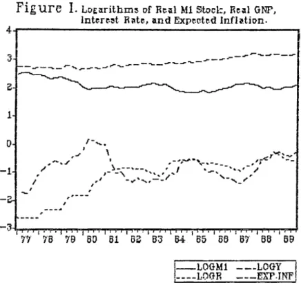
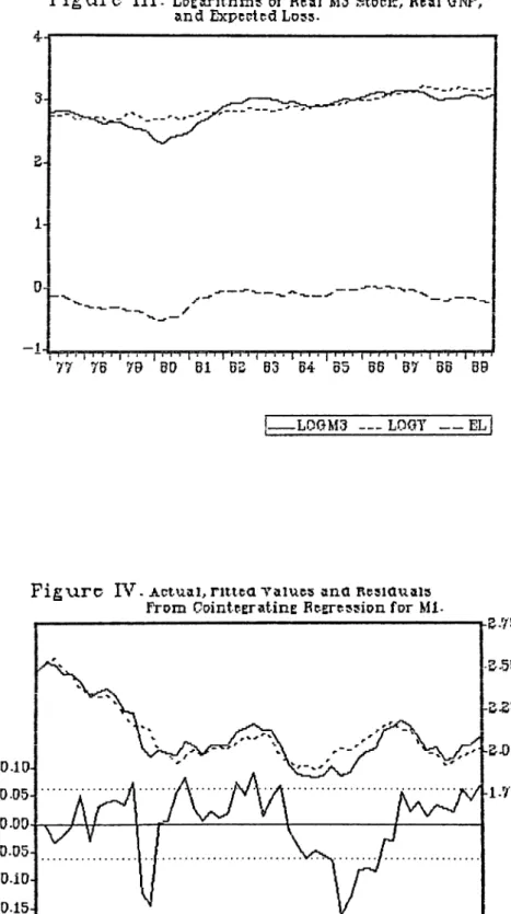
The examination of figures I, II, and III which plots the
variables show a long-run equilibrium relationship. Although
there logarithms of the time-series of interest indicates that
the are some short run deviations, they show a common trend in
the long run at least for the concerning 13 years.
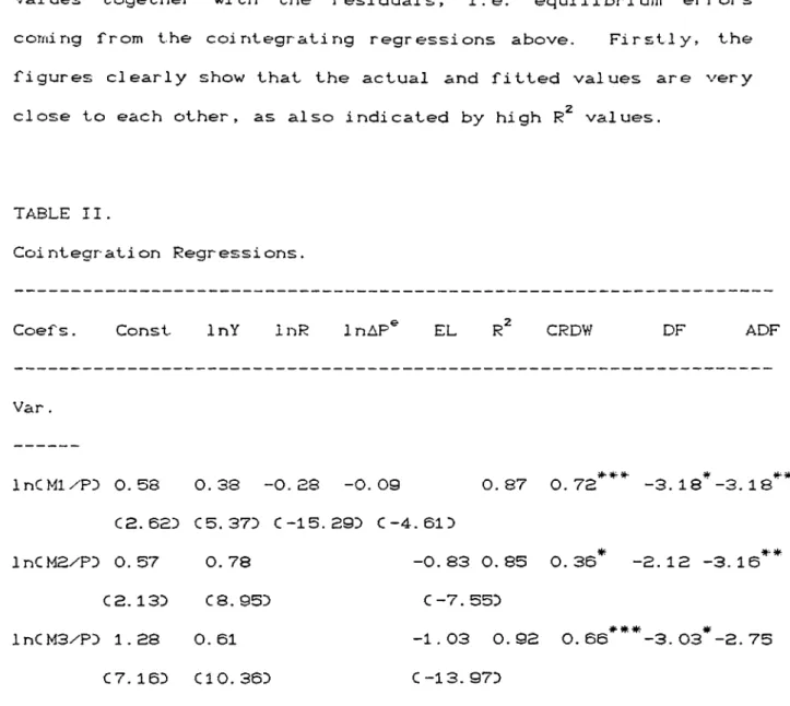
The figures IV, V, and VI, plots the actual and fitted
values together with the residuals, i . e. equilibrium errors
corning from the cointegrating regressions above. Firstly, the
figures clearly show that the actual and fitted values are very
close to each other, as also indicated by high values.
TABLE II.
Cointegration Regressions,
Coefs. Const InY InR 1пДР® EL CROW DF ADF
Var. InCMl/PD 0.58 0.38 -0.28 -0.09 C2.62D C5.37D C-15.29D C-4.61D 0.87 0.72 -3.18 -3.18 lnCM2./PD 0.57 C2. 13D C8.95D lnCM3/PD 1.28 0.61 C7.16D CIO. 36D 0.78 -0.83 0.85 0.36 -3.12 -3.16 C-7. 55Г) -1.03 0.92 О. 66***-3. 03*-2. 75 C-13. 97D
NOTE: Critlca.1 v a l u e s o f A D F a n d DF t e s t s v b v c b a r e t a k e n from H a l l <1PB<3) f o r a t h r e e v a r i a b l e c o l n t e g r a t l o n e q u a t i o n a r e a s f o l l o v s : F o r A D F , - 3 . BP, - 3 . 13, - 2 . B2 at 1, 5 a n d l O p e r c e n t l e v e l o f s i g n i f i c a n c e r e s p e c t i v e l y w h e r e a s f o r CRDW t e s t , t h e y a r e O. 4BB, O . 3<57, O. ЗОВ a t 1, 5, a n d l O p e r c e n t l e v e l o f s i g n i f i c a n c e r e s p e c t i v e l y . T h e c r i t i c a l v a l u e s f o r D F t e s t a r e a v a i l a b l e f o r two v a r i a b l e c o l n t e g r a t l o n e q u a t i o n w it h l O O o b s e r v a t i o n s . T h e y a r e a t ±96, 5%, a n d 1096 l e v e l o f s i g n i f i c a n c e - 4 . 0 7, - 3 . 37, - 3 . 0 3 r e s p e c t i v e l y . d e n o t e s s i g n i f i c a n c e at 1 96 l e v e l . ★ ★ d e n o t e s s i g n i f i c a n c e at 5 96 l e v e l . ^ d e n o t e s s i g n i f i c a n c e at l O 96 l e v e l .
Figure I.
LoEarithms of Rtal Ml Stoclz, Real GNP, Interest Rate, and ExpectedInflation-• ) J I ."r . . M j Pi i I'rri , T r > j i rt'{ i i J ^ f t . | Ti·^ ;■■ rj" i~ T"r"P
77 7B 79 50 51 5S 53 54 55 56 57 55 69
LOGMl --- LOGY
--- LOOK --- EXP-INF
Pig\.ire II-
Locwiih.me o€ R^RlMS Stack, Rc*il GNP,and Expected
Figure III.
LoERTithms of Real M3 Stock, Real GhT, and Expected Lose.Pigxirc IV -
Actual,ritica
"values ana Resiauais From CointcEratinE RcEression for Ml·hB-75
•50
£5
•OD
1-V5
Pigtirc V-
Actual, n u ca vaiucí ana Rc5>iauai3From CcintcEratinE EcETcssicn fo r MB.
-RESIDUAL -AQTUAL - — FITTED
Figure VI-
Actual, nttca values ana Rcsiauals-RESIDUAL -ACTUAL — FITTED
Secondly, the examination of the residuals reveals the fact that
they are stationary indicating the cointegration relation for
the concerning variables.
In sum. Identifying long run money demand for different
definitions of money is approached by searching for common
trends between the corresponding determinants of them. They are
real GMP, expected inflation rate, and nominal interest rate for
time deposits for real Ml stock whereas they are expected loss
term and real GHP for M2 and M3 stock of real balances.
Cointegration regressions suggest that all the three real
monetary aggregates has a long run trend relationship with the
corresponding determinants of them. The cointegration
regressions measure the long run equilibrium relationship
betv/een these variables and the the short run deviations from
this long run equilibrium relationship is accounted by the
residuals from these regressions.
The observations about the long run magnitudes of the
cointegration vectors are in order. A closer look at table II
will reveal the fact that all of the long run coefficients of
the real income surprisingly reject the hypothesis that it is
statistically equal to unity. The tests of significance,
however,, are rejected at high levels of significance. This
finding of long run coefficient of real income not equal to
unity suggests that the classical vision of the neutrality of
money is consistent with the Turkish experience at least for 13
Coining to the coefficient of the interest rate on time
deposits, it is observed that it has a negative impact on Ml
definition of money indicating, as I have already noted, that
it represents the opportunity cost of holding real balances for
Ml. On the other hand, EL term has a negative coefficient for
both M2 and M3 definitions of money reflecting the fact that it
represents the opportunity cost of holding M2 and M3 real
balances.
The expected inflation rate, as expected, has a negative
coefficient for Ml. One remarking observation is that the
effect of a one percent increase in inflation on the demand for
money is less than that of an increase in the interest rate.
This result contradicts the previous findings supporting
generally even the insignificance of the interest rate CKeyder,
19882>D for the period before 1980s. This may be explained by
the effectiveness of the liberalization efforts of the financial
structure of Turkey after 1980.
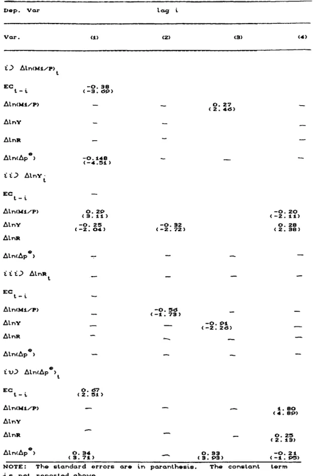
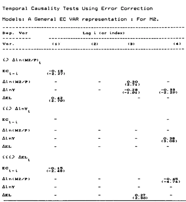
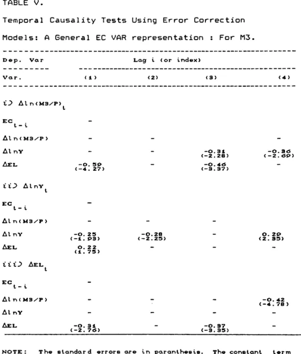
CD The Error Correction Models :
As explained before, the VAR EC modeling involves the
regressing the first difference of each variable onto lagged
values of first differences of all the variables plus the lagged
value of the error correction term. However, the choice of the
lag lengths to be used in the ECM becomes a major issue. Here,
HoTidry* s general to specific mod^lin^ strate^^y is found to be
convenient due to its simplicity Csee Gilbert C1986DD. Firstly,
ECMs with four lags of each variable Cfor quarterly data is
usedD are estimated. Later, the lags with insignificant
coefficients are elinriinated and then the newly specified model
is estimated. The same strategy is followed for each of the
three monetary aggregates and the results are reported in Tables
III, IV, and V.
Having a closer look at tables III, IV, and V will give us
several interesting temporal causality interpretations. The
sign of the coefficient of EC term from the cointegration
regression is negative for AlnCMl/PD, AlnCMS/'PD, AlnCMS^'TD, and
EL; and positive for AlnY. The temporal causality
interpretation of such a finding can be figured out as when the
money supply exceeds the money demand, that is the long run
steady state path of the economy is interrupted and there
occurred an equilibrium error, the the growth rate of the
expected loss and that of money supply should fall whereas the