Domestic saving and tax structure: Evidence from Turkey

(1)

Domestic Saving and Tax Structure: Evidence from Turkey

Article in Sosyoekonomi · January 2015

DOI: 10.17233/se.48977 CITATIONS 2 READS 419 1 author:

Some of the authors of this publication are also working on these related projects: 7th International Conference of Political Economy (ICOPEC 2016) View project

Research articlesView project Savas Cevik

Selcuk University

40PUBLICATIONS 102CITATIONS

SEE PROFILE

All content following this page was uploaded by Savas Cevik on 01 February 2015.

(2)

Sosyo

Ekonomi

January-March 2015-1

Domestic Saving and Tax Structure: Evidence from

Turkey

Savaş ÇEVİK scevik@selcuk.edu.tr

Yurtiçi Tasarruflar ve Vergi Yapısı: Türkiye Örneği

Abstract

The impact of tax policy and tax structure on national saving level is an important question for both macroeconomic stabilization and growth purposes, for especially developing countries. This paper examines the impact of tax structure on domestic saving for Turkey through cointegration and vector error correction models from 1965-2011 annual data. The results indicate that there are unidirectional Granger causalities to domestic saving from variables on tax for short-run coefficients. For the long-run, taxes on income as a share of total tax revenue found to be having negative impact on domestic saving, while the ratio of consumption taxes to total tax revenue found to be having negative impact on domestic saving. While the results are consistent with theoretical literature, they may be expected to contribute to empirical discussion of design the tax policy on developing countries and Turkey where do not have enough empirical finding in the field.

Keywords : Domestic Saving, Tax Structure, Tax Mix, Tax Policy, Vector

Error Correction.

JEL Classification Codes : E21, E62, H30.

Özet

Ulusal tasarruf düzeyi üzerinde vergi yapısının ve vergi politikasının etkisi, özellikle gelişmekte olan ülkelerde makroekonomik istikrar ve büyüme açısından önemli bir sorundur. Bu çalışma, 1965-2011 dönemi verisi ile eşbütünleme analizi ve vektör hata düzeltme modelleri aracılığıyla yurtiçi tasarruflar üzerinde vergi yapısının etkisini analiz etmektedir. Kısa dönem katsayılardan elde edilen sonuçlar vergi değişkenlerinden yurtiçi tasarruflara doğru tek yönlü bir Granger anlamda nedenselliğin bulunduğunu göstermiştir. Uzun dönem ilişkisi ise gelir üzerinden alınan vergilerin toplam hasılat içindeki payının tasarruflar üzerinde negatif, tüketim üzerinden alınan vergilerin toplam hasılattaki payının ise pozitif etkiye sahip olduğunu göstermektedir. Bu sonuçlar teorik beklentilerle tutarlı olduğu gibi, konuyla ilgili yeterli ampirik bulgu olmayan Türkiye gibi gelişmekte olan ülkelerde vergi politikası ve vergi sisteminin tasarımı ile ilgili tartışmalara katkıda bulunması beklenmektedir.

Anahtar Sözcükler : Yurtiçi Tasarruflar, Vergi Yapısı, Vergi Karması, Vergi Politikası, Vektör Hata Düzeltme Modelleri.

(3)

(4)

89 1. Introduction

Individual decisions on work, save, invest and consume are affected by taxation, in its various forms. The dimension of these effects varies due to tax mix and tax structure as well general level of tax burden. With respect to fiscal policy, whether tax policy may be a tool for promoting the economic performance is an important issue for researchers and policy-makers.

One of main aims in the tax reforms has been to improve the economic incentives on capital formation and economic growth as well fairness and some social goals. Throughout the last thirty years, most countries has attempted to tax reforms which regarding to decrease tax rates on capital income and to enhance consumption taxes to encourage economic growth through increasing investments. To achieve this goal, relative importance of taxing income or consumption in the tax structure has been debated by scholars for a long time.

Taking into account the fact that savings are a key matter of economic growth and performance1_{, one should analyze how important are influences of tax system on savings.}

This matter is especially important for developing countries which are dependent on foreign savings to finance the development since they do not have enough domestic savings. Furthermore, increasing financial opening after 1990s has decreased the level of domestic saving in developing countries (Aizenman et al. 2009). Turkey, also has suffered the low domestic saving rates, like most of developing countries for a long time. The low level of domestic saving reduces economic growth or makes economies more dependent on capital imports to maintain investments. More importantly, recently the low level of domestic saving has created the hazardous level deficit in Turkeys’ current account in consequence of increasing foreign savings to finance capital account (Rodrik, 2009). Nowadays, an important concern about Turkish economy has been that high level of the current account deficit leaves the economy vulnerable to the market shocks. However, declining saving rates are not only a problem for developing countries. Most developed countries also have experienced a declining in saving rates for the past quarter of the century.

Therefore, the factors that determine the savings have been analyzed in an extensive literature. Studies have demonstrated that besides some main determinants such as income, interest rate, the level of prices and demographic characteristics, fiscal policy and taxation are also important factors that have impact on the level of saving. This study focuses on the impact of tax structure on the domestic savings, in case of Turkey. Although there

1_{Aghion et. al., (2009) has displayed that a country’s ability to take advantage of international technology}

diffusion, is positively correlated with the level of its domestic savings. In particular, for developing countries, an increase in the domestic saving leads to an important increase in average future growth rate.

(5)

90

has been a great discussion about saving rates, economic performance and possible changes in the tax structure, there are little empirical finding related to developing countries, and especially to Turkey. Whereas, it is empirically be known that there are considerable differences between industrial economies and developing countries with regard to responsiveness of domestic saving to fiscal policy changes (Lopez et al., 2000).

The paper seeks to examine the relationship between national saving and alternative taxes (mainly income and consumption taxes), and to provide empirical evidence from Turkish macroeconomic data. For these aims, it first reviews the theoretical and empirical literature on relationships between saving and taxation. Later, it gives an overview of Turkey’s national saving problem and Turkey’s tax structure. And finally, it empirically analyze the impact of tax mix on domestic saving through cointegration analysis and vector error correction models based on 1965-2011 time series data of Turkey.

2. Effects of Tax Structure on Saving: A Theoretical and Empirical Survey Tax structure that consists of relative weights of individual taxes alters the incentives to save or to consume. While an income tax reduces disposable income (Y) as well the tax rate (ty), one can expect that the portion of the income which allocate to saving

(S) and consumption (C) falls. On the other hand, that’s why a consumption tax raises the cost of purchasing a consumption bundle as well the tax rate (tc), it does not fall on saving

and therefore investments. Thus, at a simple setting, the relationship of tax mix to the tax base is can be shown as following:

𝑌(1 − 𝑡𝑦) = 𝐶(1 − 𝑡𝑐) + 𝑆 (1)

Taken into account the interactions between savings, investments and the economic growth2_{, one of the main goals of tax reforms which aimed at reducing taxes on}

income and gains is to provide incentives economic activities through more saving. Of course, the lower income taxes also promote consumption as well saving, but consumption taxes alter composition of income allocated between savings and consumptions in favor of the savings.

However, the effects of taxation on saving and consumption are more complex than this simple setting, since income tax is imposed on return on saving (income from capital) as well earned income. For a neoclassical intertemporal consumption model with two periods and competitive markets3_{, the present income (Y}

1) equals the sum of the present

2_{For a discussion on the correlation of saving and investment see. Devereux, (1996).}

(6)

91 consumption (C1) and savings [Y1 = C1 + S], while consumption is limited by income in

that period plus saving with return of saving (r), for the second period [C2= Y2 + S (1 + r)].

The present value of consumption must be equal to the present value of income, if intertemporal budget constraint is written as following:

𝐶1+ 𝐶2⁄1 + 𝑟= 𝑌1+ 𝑌2⁄1 + 𝑟 (2)

Since an income tax reduces the return on saving, one can expect that it would have a substitution effect in favor of the present consumption (Eq. 3). On the other hand, an indirect taxation on goods instead of an income tax would raise the price of consumption from 1 to (1+tc) (Eq. 4). 𝐶1+ 𝐶2 1+𝑟(1−𝑡_𝑦)= 𝑌1(1 − 𝑡𝑦) + 𝑌₂(1−𝑡_𝑦) 1+𝑟(1−𝑡_𝑦) (3) (1 + 𝑡𝑐)𝐶1+ (1+𝑡_𝑐)𝐶₂ 1+𝑟 = 𝑌1+ 𝑌₂ (1+𝑟) (4)

It can be seen from this simplified model that a tax mix change toward the less income tax and more consumption tax would reduce the present-term consumption and therefore increase saving, with given present-term income. Increasing after return on saving would create a substitution effect. Consequently, the structure of the tax system may influence saving both by changing lifetime wealth and, by affecting the rate of return on saving. While a tax on consumption leaves unaltered the relative price of present and future consumption, an income tax on the return on saving distorts the intertemporal resource allocation by increasing the price of future consumption. Furthermore, at a macroeconomic level, an income tax has further implications on saving. High-income households are affected more by income taxes, since income taxes are generally progressive and household saving rates are also progressive related to income (Callen and Thimann, 1997).

It is as generally accepted from other studies and simulations (e.g., Summer, 1981; Auerbach and Kotlikoff, 1983; Kotlikoff, 1984; Sandmo, 1985) on this neoclassic intertemporal optimization model is that lowering taxes on capital income reduce current private consumption not only through substitution effects associated with the higher price of current relative to future consumption, but also through income effects associated with the reduced present value of a household’s human capital endowment.

However, it should be noted that since higher after-tax return on saving by changing of tax mix can create an income effect which means that consumers can use raised sources to current consumption as well as saving, the overall impact of reducing income taxes on saving remains unclear. Furthermore, the effect of tax system on saving don’t work uniformly, while some provisions may increase saving incentives as well others reduce

(7)

92

saving incentives. The tax system effects saving not only through tax mix, but also tax treatment on individual retirement accounts and capital gains is matter. Most industrialized countries have tax incentives for certain types of savings (such as owner-occupied housing, private pension funds) over others (such as bank deposits) to increase growth by reducing distortions at saving behaviors (Johansson et al., 2008). Studies demonstrate that tax-deferred saving accounts have induced massive portfolio shifts towards tax-favored assets (Poterba, 2001; Jappelli and Pistaferri, 2003).

On the other hand, changing tax mix with respect to reduce income taxes does not affect by similar way all groups in a society. We can expect that since low-income households have a tendency of low saving, reducing income taxes would probably stimulate increasing in consumption for these income levels on the contrary of high-income households (Garner, 1987). Nevertheless, arguments of this neoclassic model with rational consumer have been driving the tax reforms, toward reducing income taxes to promote economic performance, which throughout 1980s and 1990s. Proposes on cutting in income taxes by supply-side economists of U.S. had depended on these arguments which tax cuts raise the after-tax incentives to work, save, and invest.

While its proposals on tax mix are rarely criticized, the model comes under attack concerns the validity of assumptions on rational consumers operating with perfect capital markets and their simplified saving motives. First of all, there are many different motives for saving and an heterogeneity in types of saving, such as Keynesian precautionary purposes, speculative reasons, providing resources for retirement and bequests and deposing for large possible consumption items, while there is the gap between interest rates for saving and borrowing in real economies. Therefore, household may not respond to small changes in after-tax return on saving (Freebairn, 1991; Boadway and Wildasin, 1995).

A numerous studies have employed the after-tax interest rate as a proxy measure of the return on saving, to consider an effect of taxing. However, the empirical evidence presents ambiguous results. For example, Hall (1988) found no effects of interest rates on savings. Bovenberg (1989) argued that the effects of taxes on private savings is relatively small and uncertain, while public saving has direct impact on national savings in the US. However, he accepted that the tax system powerfully affects the composition of savings and investments. One influential study by Boskin (1978) found a substantial sensitivity of saving to after-tax return. Gylfason (1981) also found similar results with Boskin (1978). Other studies (Howrey and Hymans, 1978; Hall, 1985; Blinder and Deaton, 1985) found little sensitivity of saving to the rate of return or no significant effect of after-tax return. Attanasio and Banks (1998) have found from their examination on UK and US that there are little evidences the fact that tax incentives to promote national saving. They concluded that tax incentives to stimulate saving has probably mistargeted, if their aim is to increase saving rates. However, the results from empirical studies point out the controversial findings and have not provided definitive evidence on the sensitivity of saving to after-tax returns because

(8)

93 of probably quite different statistical models adopted (Honohan, 2000; Jappelli and Pistaferri, 2002; Loayza et al., 2000). Tanzi and Zee (1998) argued that inconclusiveness of the empirical results is probably due to the fact that differences in data sets used, differences in definitions of saving, and moreover, most studies heavy relied on the United States where may be characterized by stable tax structure over decades and by occasional important change in tax provisions.

In one of rare studies that use tax mix indicators as explanatory variables, Callen and Thimann (1997) found the ratio of direct taxes to total government revenue to have a significant negative impact on saving, while the indirect tax ratio is significant, from panel data for OECD countries. Tanzi and Zee (1998) found from data of OECD countries that the ratios of total tax revenue, income tax revenue and consumption tax revenue to GDP are statistically significant and negatively relationship to the household saving rate. Furthermore, negative coefficients for income taxes are especially higher than those for consumption taxes. They have also found that when the total taxation as a share of GDP is held constant, household saving rate bears a positive and statistically significant relationship to consumption taxes that this finding could be interpreted as the positive effect on the saving behavior of replacing income with consumption taxes.

Although most studies on determinants of saving are on developed countries, several studies from data on developing countries also provide evidences for negative impact of taxation (especially those of income taxes), as results vary by individual countries. Jenkins (1989) displays that changing in tax structure toward indirect taxes from direct taxes in Sri Lanka has increased the gross capital formation. Cardenas and Escobar (1998) pointed out that general level of taxation negatively affects private savings for Colombia. Dahan and Hercowitz (1998) found that income taxes in Israel are negatively related to saving rates. Kerr and Mongish (1998) have reported that direct taxes have a negative impact on saving in India. For Turkey, Fletcher et al. (2007) found as statistically insignificant the real interest rate which indicates the after-tax return on saving. Değirmen, S. and Şengönül A. (2012) has employed the net tax ratio (total tax revenue minus transfers as a share of GDP) as a regressor, but they have no found a statistically significant coefficient on the variable.

3. Saving and Tax Structure in Turkey: Motivation for the Study

It is widely accepted that the saving provides resources for private capital formation and in turn, raises economic growth and productivity. For the society, a larger capital stock enhances the aggregate output and income per capita. Especially for developing countries who strains to obtain high economic growth and development, higher domestic

(9)

94

saving is needed to spur domestic capital formation without continued reliance on foreign saving4_.

In recent years, one of the most important economic problems of Turkey is pressure which created by low household saving rates and large current account deficit. Since Turkey has low saving rates in international levels, its high growth rates are financed by foreign savings, and in turn, and this economic structure increases current account deficits. As shown in Figure 1, domestic savings in Turkey have continuously declined since the late 1980s despite of temporary increasing in the course of 1997-99. Although the fall in the saving rate was driven by the public sector deficits throughout 1990s, post- 2001, it is due to declining in private savings (World Bank, 2012). In comparison with the other countries, it can be seen that Turkey has considerably lower saving rates among comparable income levels. The countries with upper middle level –that Turkey also is member of this category-, who have high growth rates, follow a contrast path with Turkey after 2000s. If Turkey’s high growth rates and high current account deficits are taken into account after 2001, it is understood from the Figure 1 that Turkey has financed its growth with foreign capital inflows. The low level of saving rates and its dependency on external financing not only put at risk the sustainability of investments and economic growth of Turkey, but also it creates a pressure on the economy with respect to possible volatilities in the capital flows.

As known from the previous section, tax structure and tax provisions of the country are important variables to explain behaviours saving and consumption. Undoubtedly, special tax provisions (on retirement funds or financial investments) and after-tax return rates on saving could be more explanatory to examine causality relationships. However, the effect of taxation on saving can be approached through the changing tax mix at a macroeconomic setting, if one would like to investigate effects of the government’s financing structure. A tax mix would reflect aggregated effects of individual tax provisions. Taken into account that a bulk of studies5_{finds empirical evidence for the link between tax}

mix and economic performance and individual types of taxes have different effects on economic behaviours, to change the tax mix can be a policy instrument as well an examining tool for economic effects of taxation. Tax reform initiatives attempt to change the tax mix in favour of an individual type of tax according to aimed efficiency and equality, ultimately.

4_{However, it should be noted that there are ambiguous empirical findings on the association between the growth}

and national saving for developing countries. For Turkey, Yentürk et al, (2009) has detected bidirectional Granger causality toward private sector savings from GNP, and concluded that increasing private savings do not help initiating growth and investment in Turkey like some other developing countries have excess capacity. On the other hand, Değirmen and Şengönül (2012) recently found that economic growth and public investments positively affects the private savings rates in Turkey.

(10)

95 Figure: 1

Gross Saving Rates (% GDP): Turkey and Countries by Income Group

For the last quarter century, the main pattern in tax reforms at OECD countries is to change tax structure towards flatter personal income tax, cutting corporate tax rates, and decreasing overall top marginal rate on dividends6_{. It is widely accepted personal and}

corporate income taxes to have biases against savings and capital formation. Despite cross-country differences in the tax structure, it can be said that while countries has a tendency of reducing taxes on income for economic growth goals, global pressures (tax competition to attract capital, increasing indirect environmental taxes, etc.) force to increase indirect taxes from goods and services in most OECD countries, recently. On the other hand, Turkey like most developing countries has tax structure depending on indirect consumption taxes (Figure 2). Developing countries prefer indirect taxes because of political and administrative

6_{Two special cases for reforms on this way are the dual income taxes in Nordic countries and the flat-rate income}

taxes in Baltic and former Soviet countries that both of them aim at promoting capital and undermine traditional income taxes with progressive rate and with global structure.

0 5 10 15 20 25 30 35

Turkey Upper-Middle Inc.

OECD - High Inc. Lower-Middle Inc.

(11)

96

constraints as well to promote economic growth. It is commonly accepted that since indirect taxes has negative distributional results, developing countries should transform their tax structure into one which weighted income taxes. Undoubtedly, there is a trade-off between economic efficiency and fairness. The possible tendency for many developed countries is also to use indirect taxes to finance the government in consequence of the goal of strengthening the economic performance.

Figure: 2

Tax Structure in Turkey and OECD

4. Data, Empirical Analyses and Findings

4.1. The Data and Econometric Procedure

Taken into account initiatives of tax reform aimed at change tax mix, the empirical analysis of the study focus on examining the causality and the impact of tax structure on domestic saving in Turkish case. Accordingly, it will be used the ratios of income taxes and consumption taxes to total taxation and overall tax burden of economy (the ratio of total tax revenue to GDP) as tax variables. It is possible that tax structure may affects public saving and private saving in different directions. Again, it is probable that there could be an interaction (such as the effect of crowding out) between public and private saving levels such as proposed by the Ricardian equivalence hypothesis (Barro, 1974).

0 10 20 30 40 50 60 OECD - Tax Revenue (%GDP) Turkey - Tax Revenue (%GDP) OECD - Taxes on Income (% Total Taxes) Turkey - Taxes on Income (% Total Taxes) OECD -Consumption Taxes (% Total Taxes) Turkey -Consumption Taxes (% Total Taxes) 1970 1980 1990 2000 2010

(12)

97 Although World Bank (2012) estimates as very small the Ricardian offset coefficient (the percentage decline in private saving as a result of a one percent increase in public saving) in Turkey7_{, it is possible that public savings could be affected by changing in tax mix because}

of differences at revenue-extracting abilities of individual taxes. Since the study interests in aggregated effect of taxation on Turkey’s saving level, it uses per capita domestic saving comprised both private and public saving as the indicator to saving level. From theoretical and empirical examinations in the previous section, we expect that increasing in share of indirect consumption taxes in tax structure may be associated with increasing in saving level, while level of income taxes could decrease saving levels. We hypothesize that since consumption taxes apply the same tax rate on current and future consumption they do not influence the rate of return on savings and individual’s savings choices as income taxes do. Hence, consumption taxation may be favoring saving levels relative to income taxation.

The long-run aggregate saving model of an economy can simply be characterized by following general function for empirical aims.

𝑆𝑡= (𝑌𝑡, 𝑅𝑡, 𝑇𝑡) (5)

where S is aggregate saving, Y is national disposable income, R is interest rate as a proxy of return on saving and T is a variable on taxation. Relying on this base empirical framework, it will be estimated following log-linear models (Eq.6, 7 and 8) in order to investigate effect of tax mix variables on saving.

𝑴𝒐𝒅𝒆𝒍 𝟏: 𝑙𝑛𝐿𝑃𝑆𝐴𝑉𝑡= 𝛼 + 𝛽1 𝐿𝑃𝐺𝐷𝑃𝑡+ 𝛽2𝑅𝑡+ 𝛽4𝑇𝐴𝑋𝑡+ 𝑢𝑡 (6) 𝑴𝒐𝒅𝒆𝒍 𝟐: 𝑙𝑛𝐿𝑃𝑆𝐴𝑉𝑡= 𝛼 + 𝛽1 𝐿𝑃𝐺𝐷𝑃𝑡+ 𝛽2𝑅𝑡+ 𝛽4𝐼𝑁𝐶𝑇𝐴𝑋𝑡+ 𝑢𝑡 (7) 𝑴𝒐𝒅𝒆𝒍 𝟑: 𝑙𝑛𝐿𝑃𝑆𝐴𝑉𝑡= 𝛼 + 𝛽1 𝐿𝑃𝐺𝐷𝑃𝑡+ 𝛽2𝑅𝑡+ 𝛽4𝐶𝑂𝑁𝑆𝑇𝐴𝑋𝑡+ 𝑢𝑡 (8) As an indicator to saving, it was employed the gross domestic saving per capita (LPSAV) that has calculated by dividing population gross real domestic saving obtained World Bank, World Development Indicators after it was deflated with GDP deflator. Explanatory variables are per capita real GDP (LPGDP) calculated from data obtained the Turkish Ministry of Development and the Turkish Statistical Institute, the discount rate (R) as a proxy of interest rate that obtained IMF International Financial Statistics, and tax variables as the ratio of total tax revenue to GDP (TAX), the ratio of income taxes to total tax revenue (INCTAX), and the ratio of consumption taxes to total tax revenue (CONSTAX). Tax variables were drawn from OECD Tax Database with exception of the ratio of tax

7_{Özcan et al. (2003) had found that an increase in the public saving rate by one percentage decreases the private}

(13)

98

revenue to GDP which has been calculated by data from Turkish Revenue Administration. The data on income taxes consist of personal income tax and corporate income tax, while the data on consumption taxes comprise of sum of general sales taxes (i.e. value added tax), excise taxes and taxes on international trade - customs. LPSAV and LPGDP were used by their logarithmic transformations in analyses by following the related literature.

The estimations were performed on annual observations for period 1965-2011. Although using annual data is be criticized with respect to a satisfactory degree of freedom, in order to obtain quarterly data with high frequency is also difficult for all variables in Turkey case. On the other hand, since quarterly data is required seasonally adjusting that could distort temporal relationship between variables, it may also be undesirable. Furthermore, as noted by Hakkio and Rush (1991) having a long time span rather than a high frequency of observations could be more important, especially if one interests in causality relationship.

Basic econometric strategy adopted in empirical analyses is as following: Firstly, variables were tested for the unit root, since it is known the fact that many economic time series are not stationary. In the second step, equations were tested for cointegration. Since each of three equations was found the cointegrations relationship, the vector error correction models were constructed to analyze causality for both short and long term between domestic saving and tax variables. This procedure was separately followed for each of the models (Eq.6, 7 and 8). We especially interest in differences between results from Model 2 and Model 3.

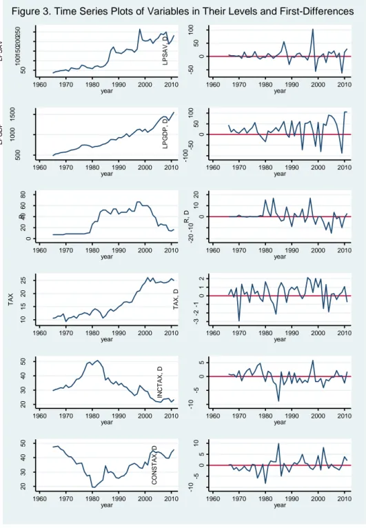
4.2. Testing for Unit Roots

Since non-stationary series could generate a spurious regression and the econometric methods which will be choice depend on integration level of variables, it is be required variables to be tested for unit root. A unit-root process is one that is integrated of order one, meaning that the process is non-stationary but that first-differencing the process produces a stationary series. Figure 3 which presents time series plots of variables supports visually all variables to be non-stationary. First column of the Figure presents the time series in levels of variables, while second column displays the time series at their first differences.

(14)

99 50 100 150 200 250 L P S A V 1960 1970 1980 1990 2000 2010 year -5 0 0 50 100 L P S A V , D 1960 1970 1980 1990 2000 2010 year 500 1000 1500 L P G DP 1960 1970 1980 1990 2000 2010 year -1 0 0 -5 0 0 50 100 L P G DP , D 1960 1970 1980 1990 2000 2010 year 0 20 40 60 80 R 1960 1970 1980 1990 2000 2010 year -2 0 -1 0 0 10 20 R, D 1960 1970 1980 1990 2000 2010 year 10 15 20 25 T A X 1960 1970 1980 1990 2000 2010 year -3 -2 -1 0 1 2 T A X , D 1960 1970 1980 1990 2000 2010 year 20 30 40 50 INCT A X 1960 1970 1980 1990 2000 2010 year -1 0 -5 0 5 INCT A X , D 1960 1970 1980 1990 2000 2010 year 20 30 40 50 CO NS T A X 1960 1970 1980 1990 2000 2010 year -1 0 -5 0 5 10 CO NS T A X , D 1960 1970 1980 1990 2000 2010 year

(15)

100

Table: 1

ADF and PP Unit Root Tests

ADF Test PP Test Variable Form Lag(a) _Intercept Intercept and

trend Intercept Intercept and trend LPSAV Level (1) -0.896 -3.628** -1.342 -21.755** First difference (0) -7.755*** -7.660*** -43.575*** -43.562*** LPGDP Level (1) 1.001 -1.616 1.051 -7.046 First difference (0) -6.301*** -6.489*** -41.881*** -41.709*** R Level (1) -1.370 -0.511 -3.233 -1.240 First difference (0) -5.781*** -6.089*** -40.929*** -42.194*** TAX Level (1) -0.103 -1.916 -0.167 -6.828 First difference (0) -7.292*** -7.263*** -50.096*** -50.123*** INCTAX Level (1) -0.924 -1.988 -2.499 -5.408 First difference (0) -3.560*** -3.666** -40.619*** -42.375*** CONSTAX Level (1) -1.538 -1.665 -4.853 -4.114 First difference (0) -6.351*** -6.856*** -48.037*** -49.379***

*, **, *** indicates the significance at 10%, 5% and 1%, respectively.

(a)_{The lag selection is based on Akaike’s information criterion (AIC), Hannah and Quinn’s information criterion} (HQIC), and Schwarz’s Bayesian information criterion (SBIC).

However, obtaining the exact integration levels of the variables is only possible with formal tests. Therefore, three formal tests has been carried out for all variables as Augmented Dickey-Fuller test (ADF) (Dickey and Fuller, 1979), Phillips-Perron (PP) test (Phillips and Perron, 1988), and a modified version of Dickey-Fuller test (DF-GLS) suggested by Elliott et al., (1996). DF-GLS is a modified Dickey–Fuller t test for a unit root in which the series has been transformed by a generalized least-squares regression, and Elliott et al., (1996) have shown that this test has greater power than ADF version.

Tests of ADF and PP are reported in Table 1 and DF-GLS is in Table 2. Both tests from Table 1 indicate that all of variables are stationary in the first differences. The null hypothesis of a unit root is rejected for the variables at the 1% significance level. However, tests with constant and trend for LPSAV shows a doubt of having unit root at the level. Therefore, DF-GLS test for unit root that is a more advanced test is applied. As can be seen Table 2, DF-GLS is not able to reject the unit root hypothesis. Therefore we conclude that all series are integrated of order one, I(1), and it is appropriate to proceed to test for the cointegration analysis.

(16)

101 Table: 2

DF-GLS Test for Unit Root

Variable Form Test Statistics Lag(a) _Decision

LPSAV Level Intercept -0.178 (1)

I(0)

Intercept and trend -3.190* (1)

First difference Intercept -5.680*** (1)

I(1)

Intercept and trend -5.624*** (1)

LPGDP Level Intercept 2.148 (1)

I(0)

Intercept and trend -1.705 (1)

I(1)

R Level Intercept -0.972 (1)

I(0)

I(1)

TAX Level Intercept 0.331 (1)

I(0)

First difference Intercept -3.656*** (1) _I(1)

INCTAX Level Intercept -0.986 (1)

I(0)

I(1)

Intercept and trend -3.333** (1)

CONSTAX Level Intercept -0.954 (1)

I(0)

I(1)

(a)_{Lags are determined by Schwarz information criterion and modified Akaike’s information criterion}

4.3. The Cointegration Analysis

Since all variables found to have stationary at their first differences, the cointegration rank can be estimated to determine the presence of a long-run relationship among the variables of each model, and the parameters from vector autoregressive models by following Johansen methodology (Johansen, 1988; Johansen and Jelius, 1990 and Johansen, 1995).

Before testing the cointegation of variables, one must determine the optimal lag length which will be small enough to allow the estimation, and which be high enough to ensure the errors to be white noise approximately. Findings for the optimal lag orders based on VAR models of equations has been reported at Appendix A, which minimize related information criterion. It was selected the optimal lag order as 4 for each of three models (VAR(4)). The AIC, the final prediction error (FPE) and modified LR test statistics confirm this lag specification.

(17)

102

By relying on lag order in underlying VAR from Appendix A, the null hypothesis of no-cointegration was tested by using Johansen trace statistics for a VAR model with both only constant and a constant and a trend. Table 3 reports the results from the cointegration analysis based Johansen trace statistic (λtrace) to determine cointegrating vectors. It is seen

from Table 3 that there are two cointegrated vectors in order to explain the long-run relation in Model 1, while it is one for Model 2 and Model 3, at the 1% significance level.

Table: 3

Johansen Cointegration Test

Constant Constant and trend Maximum

Rank Eigenvalue λtrace

5% critical value %1 critical value Eigenvalue λtrace 5% critical value %1 critical value Model 1. 0 70.7092 47.21 54.46 80.7673 54.64 61.21 1 0.58595 32.7928**** 29.68 35.65 0.60665 40.6463 34.55 40.49 2 0.40614 10.3851** 15.41 20.04 0.38099 20.0217*** 18.17 23.46 3 0.19038 1.3040 3.76 6.65 0.28138 5.8133 3.74 6.40 4 0.02987 0.12645 Model 2. 0 58.9079 47.21 54.46 77.7559 54.64 61.21 1 0.64083 14.8783*** 29.68 35.65 0.64287 33.4802*** 34.55 40.49 2 0.20886 4.8043 15.41 20.04 0.38059 12.8837 18.17 23.46 3 0.10171 0.1920 3.76 6.65 0.18364 4.1589 3.74 6.40 4 0.00446 0.09219 Model 3. 0 77.2946 47.21 54.46 84.9788 54.64 61.21 1 0.72718 21.4399*** 29.68 35.65 0.72890 28.8520*** 34.55 40.49 2 0.23199 10.0899 15.41 20.04 0.33747 11.1494 18.17 23.46 3 0.20452 0.2510 3.76 6.65 0.19332 1.9116 3.74 6.40 4 0.00582 0.04348

Therefore, we conclude that there is long-run equilibrium relationship for among variables in each of three models. It can be said that there is the one-way causality at least according to Engle and Granger (1987). Although the cointegration relationship does not point out the direction of the causality, it allows estimating of the causality relationships through a vector error correction model (VECM).

4.4. Vector Error Correction Models and Causality between Domestic Saving and Tax Structure

Since the variables are first-difference stationary and the presence of cointegration relationship in the equations, the Granger causality cannot be estimated in a simple VAR model. However, estimating of the causality between variables requires the model to be specified in VECM framework. A VECM is used to model the stationary

(18)

103 relationship between multiple time series that contain unit roots. In a VECM, the long-run relationships between the variables should converge and the short-run variations can be examined through the correction coefficients which measure the speed of adjustment between time series. A stable VECM displays that deviations from the relationship represent disequilibria that cannot persist indefinitely, since the cointegrating relationship describes the long-run relationship that links the levels of the stationary variables. VECM helps analyze how this equation systems return to equilibrium.

As pointed out by Engle and Granger (1987), if the variables are cointegrated, a VAR in first differences would be misspecified. A VAR(p) with p lags and contains the cointegration relationship can be expressed as a VECM as Eq. (9) following:

∆𝑦𝑡= 𝒗 + 𝚷𝑦𝑡−1+ ∑𝑝−1𝑖=1𝚪∆𝑦𝑡−𝑖+ 𝜖𝑡 (9)

where 𝑦𝑡 is a K x 1 vector of variables, 𝑣 is a Kx1 vector of parameters, and 𝜖𝑡 is a K x 1 vector of disturbances. 𝜖𝑡 has mean 0, and is i.i.d normal over time. Matrices of parameters

are 𝚷 = ∑ Aj− Ik

j=p

j=1 and 𝚪𝑖= − ∑ Aj

j=p

j=i+1 . If the variables yt are I(1) the matrix 𝚷 has 0 ≤ r ≤ K, where r is the number of linearly independent cointegrating vectors. Since it omits the lagged level term 𝚷𝑦𝑡−1, a VAR in first differences of variables is misspecified (Engle ve Granger, 1987).

A VECM as in Eq. (9), in fact, does not contain the deterministic trends stemmed from the mean of the cointegrating relationship or the mean of the differenced series. Because, a constant in an equation for the first-difference of a variable would represent a linear trend in the level of the variable, or a quadric time trend in the level would represent a linear time trend in the first-difference equation. Taken into account these deterministic components, a VECM is rewritten as in Equation 10:

∆𝑦𝑡= 𝜶(𝜷′𝑦𝑡−1 + 𝝁 + 𝝆𝑡) + ∑ 𝚪𝒊 𝑝−1

𝑖=1 ∆𝑦𝑡−𝑖+ 𝜸 + 𝝉𝑡 + 𝜖𝑡 (10)

Thus, a VECM may include five possible trend conditions. Eq. (10) represents a VECM contained all possible deterministic components (unrestricted trend). In second case, the trends in the levels are linear but not quadric one (𝝉 = 𝟎). In third case, the levels of the data have linear trends but the cointegrating equations are stationary around constant means (𝝉 = 𝝆 = 𝟎). In the restricted constant case, there is no a linear time trend in the levels and the cointegrating equations are stationary around constant means (𝝉 = 𝝆 = 𝜸 = 𝟎). And finally, the specification may not include nonzero means or trends. This case of no-trend assumes that the cointegratinf equations are stationary with means of zero and that the differences and the level of the data have means of zero (𝝉 = 𝝆 = 𝜸 = 𝝁 = 𝟎).

(19)

104

The results from a VECM is sensitive its trend components as well optimal lag selection and estimated rank number of cointegrating relationships. In order to determine deterministic components of our VECMs, it was performed the likelihood-ratio tests. Firstly, a encompassing model which include possible all trend components (the alternative hypothesis), then this model was tested against a nested models (the null hypothesis) sequentially.

Table: 4

The Likelihood-Ratio Tests for Deterministic Components of VECMs

Assumption LR Chi2 Probability Decision

Model 1. 𝜏 = 0 2.73 0.2554 𝜏 = 0 𝜏 = 𝜌 = 0 3.75 0.1534 𝜏 = 𝜌 = 0 𝜏 = 𝜌 = 𝛾 = 0 18.40 0.0001 𝜏 = 𝜌 = 0 𝜏 = 𝜌 = 𝛾 = 𝜇 = 0 34.40 0.0000 𝜏 = 𝜌 = 0 Model 2. 𝜏 = 0 2.08 0.5564 𝜏 = 0 𝜏 = 𝜌 = 0 0.37 0.5431 𝜏 = 𝜌 = 0 𝜏 = 𝜌 = 𝛾 = 0 17.66 0.0005 𝜏 = 𝜌 = 0 𝜏 = 𝜌 = 𝛾 = 𝜇 = 0 24.43 0.0001 𝜏 = 𝜌 = 0 Model 3. 𝜏 = 0 8.63 0.0347 Unrestricted trend 𝜏 = 𝜌 = 0 9.16 0.0572 𝜏 = 𝜌 = 0 𝜏 = 𝜌 = 𝛾 = 0 19.77 0.0002 𝜏 = 𝜌 = 0 𝜏 = 𝜌 = 𝛾 = 𝜇 = 0 50.04 0.0000 𝜏 = 𝜌 = 0

As seen in the Table 4, it was preferred the specifications with unrestricted constant from likelihood-ratio tests for each of three model. Although likelihood-ratio tests for lag exclusion were also performed to assess the possibility of trimming parameters numbers, previously determined lags (at Appendix A) were found to be suitable. In addition to these tests, diagnostic checks were performed such as the Lagrange multiplier test (LR) for autocorrelation at lag order; Jaque-Bera test, skewness and kurtosis tests for normality of disturbances; and test for eigenvalue stability8_{. Diagnostic tests have been reported at}

Appendix B. It could not been identified any significant departures from the standard assumptions.

8_{If the estimated VECM is stable then the inverse roots of characteristics Autoregressive (AR) polynomial will}

have modulus less than one and lie inside the unit circle. There will be kp roots, where k is the number of endogenous variables and p is the largest lag.

(20)

105 4.5. The Long and Short-Run Relationships from VECMs

The VECM approach allows distinguishing between short-term and long-term causality in addition to the direction of Granger causality among variables. The coefficients of correction terms (α parameters) represent how fast deviations from the long-term equilibrium, while β parameters from cointegrating equations could be interpreted as long-run relationship between variables in the model. On the other hand, the short-long-run coefficients (the matrix 𝜞 from Eq.10) present short-run relationship between variables that they could be subjected to a Wald Test to determine short-run Granger causality. Adjustment coefficients have been found to be negative and statistically significant for all three VECM models.

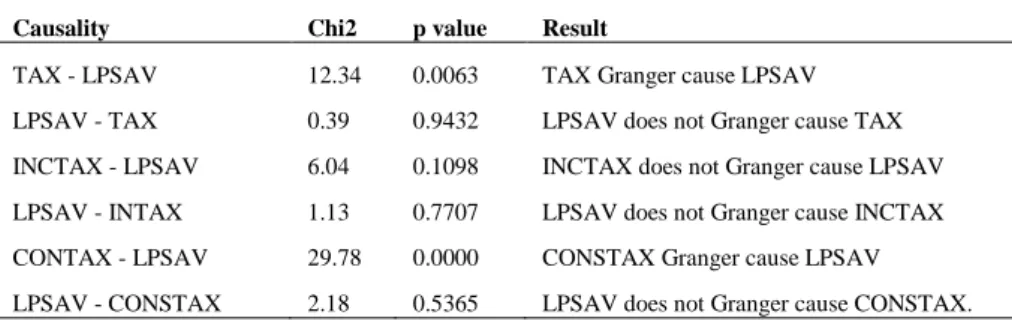
Table 6 presents short-run Granger causality between gross domestic saving and the variables on tax structure, which obtained the Wald test based on the short-run coefficients. The Wald test has been performed only for the saving (LPSAV) and tax variables (TAX from Model 1, INCTAX from Model 2, and CONSTAX from Model 3), the study interested in relationships between these variables.

Table: 6

Short-Run Granger Causality: the Wald Tests based on the VECMs

Causality Chi2 p value Result

TAX - LPSAV 12.34 0.0063 TAX Granger cause LPSAV

LPSAV - TAX 0.39 0.9432 LPSAV does not Granger cause TAX

INCTAX - LPSAV 6.04 0.1098 INCTAX does not Granger cause LPSAV

LPSAV - INTAX 1.13 0.7707 LPSAV does not Granger cause INCTAX

CONTAX - LPSAV 29.78 0.0000 CONSTAX Granger cause LPSAV

LPSAV - CONSTAX 2.18 0.5365 LPSAV does not Granger cause CONSTAX.

It is apparent from Table 6 that the Granger causality between LPSAV and variables on tax is unidirectional and toward LPSAV from tax variables. However, there is no Granger causality between saving and income taxes. As it is be expected from theoretical empirical considerations in previous sections, there are significant results of Granger causality between domestic saving and taxes on consumption and overall tax burden for even short-term.

Table 7 reports the long-run equilibrium relationships obtained from error correction coefficients for each model. All coefficients in the equations are significant at %1 level. Even though the coefficients vary among the models, in general, the long-run coefficients for per capita GDP and interest rate are positive and statistically significant as

(21)

106

expected. The coefficients for GDP can also be interpreted as the elasticity, since the variables LPSAV and LPGDP have been used in their logarithmic forms in the analyses.

Table: 7

Long-Run Relationships from Cointegrating Equations

MODEL 1. LPSAV= 1.858*R + 8.313*TAX – 2.267

(.3473065) (1.430986) MODEL 2. LPSAV = 0.1799*LPGDP + 1.070*R – 0.886*INCTAX – 27.352 (.0070395) (.0897957) (.2316404) MODEL 3. LPSAV = 1.828* LPGDP + 1.402*R + 1.375*CONSTAX – 122.67 (.0050867) (.0870442) (.1869351)

Standard errors have been reported in brackets.

Turning to variables on tax structure, interestingly, there is positive relationship between overall tax burden (total tax revenue as a share of GDP) and domestic saving. This finding can be understood if results for Model 3 and the main characteristics of Turkish tax structure are taken into account. Because, results for Model 3 used consumption taxes as tax variable indicate that there is a positive association between domestic saving and the share of consumption taxes in the total tax revenue, and as known that Turkish tax system is heavily depend on consumption taxes. Thus, the positive association between domestic saving and total tax revenue may be stemmed from this phenomenon. More importantly, results for tax structure are consistent with hypothetical expectations and findings of previous studies. In the long-term, the share of taxes on income to total tax revenue has negative impact on domestic saving (Model 2), while the share of indirect taxes on consumption to tax revenue has a positive impact on domestic saving (Model 3). For the related sample, this finding supports theoretical considerations on effects of taxation on saving as well efforts on policy design about tax reform.

Although indirect consumptions taxes are a justifiable cause of concern due to their regressive effects on income distribution, they have positive impact on saving relative to income taxes. In fact, this impact of consumption taxes can be seen as related to income distribution itself. As known, saving tendency is also related to household’s income level. One can expect that households with high income have high saving rates, while households with low income level have high consumption tendency. Findings from the recent studies which based on Turkish micro-data by Rijckeghem and Üçer (2009) and Aktaş et al., (2012) also support this fact. A tax structure heavily depended on consumption tax may be increasing total domestic saving by distorting income distribution at the same time, household with high income has been encouraged in consumption taxes instead of income

(22)

107 taxes. On the other hand, decreasing in consumption taxes could only promote household with low income to consume more, they still need basic consumption goods.

5. Conclusion

The study examines the impact of tax structure on domestic saving in Turkey by using cointegration and vector error correction models. Three equations were estimated and the variables in all equations found to be cointegrated. For all equations, it has been found per capita GDP and interest rates to have the positive impact on domestic saving. From Model 1, overall tax burden found positively related to domestic saving. From Model 2 and Model 3, the share of consumption taxes as the percentage of total tax revenue is positively related to gross domestic saving, while the share of income taxes as the percentage of total tax revenue is negatively related to gross domestic saving, for a long-term relationship. The short-run Granger causality imposes unidirectional causality toward saving from tax system, except for the variable on income taxes. These findings may support the reform initiatives of reducing income taxes to promote economic performance throughout the world, and the fact that consumption taxes are favor of saving. Undoubtedly, design of tax mix also depends on other policy priorities such as redistribution, but findings point out that a change in tax mix in favor of indirect consumption taxes rather than income taxes (personal or corporate) may create an increasing in national saving rates in case of a developing country. However, it should be noted that in Turkey, indirect consumption taxes already play a very important role in tax revenues. It is possible that the further increasing of consumption taxes in the tax system would create heavy distortions and economic costs especially with regard to distributional issues. But, the results of the study also imply that a changing in tax mix toward income taxes could impose costs related to domestic saving.

Nevertheless, these findings need to be interpreted with caution due to the study’s limitations. First of all, the analysis does not distinguish the effect of discretionary fiscal policy from changing of tax revenues caused by business cycle. It is obvious that conversions in tax structure may due to discretionary changes of the legal components (rate, deductions, credits etc.) of related tax as well changes at macroeconomic base (such as national disposable income or household consumption level) of any individual tax. Therefore, an exact policy suggestion can be drawn an analysis whose data should be corrected according to these two sources of changing. Future research should be done to investigate the effects of discretionary tax policy. Another issue is the fact that the previous studies has displayed that empirical results are sensitive to definition of saving as well statistical methods adopted. We employed the gross total domestic saving to considerate tax policy options and to investigate the impact of tax system in case of Turkey’s low saving rate, however, household saving or private saving also could use to investigate different dimensions of the subject. It should be noted that Turkey has not data on household saving for long time series, even

(23)

108

though private saving can be obtained. Finally, results have been obtained from annual observations.

References

Aghion, P. & D. Comin & P. Howitt & I. Tecu (2009), “When Does Domestic Saving Matter for Economic Growth?”, Harvard Business School Working Paper, No. 09-080. Aizenman, J. & B. Pinto & A. Radziwill (2009), “Sources for Financing Domestic Capital – Is

Foreign Saving a Viable Option for Developing Countries”, Journal of International

Money and Finance, 26, 682-702.

Aktaş, A. & D. Güner & S. Gürsel & G. Uysal (2012), “Structural Determinants of Household Savings in Turkey: 2003-2008”, BETAM Working Paper, No.07, Bahçeşehir University Center for Economic and Social Research, Istanbul.

Attanasio, O. & J. Banks (1998), “Trends in Household Saving Don’t Justify Tax Incentives to Boost Saving”, Economic Policy, 13(27), 547-583.

Auerbach, A.J. & L.J. Kotlikoff (1983), “National Savings, Economic Welfare, and the Structure of Taxation”, in M. Feldstein (ed.), Behavioral Simulation Methods in Tax Policy Analysis, Chicago: University of Chicago Press, 459-493.

Barro, R.J. (1974), “Are Government Bonds Net Wealth?”, Journal of Political Economy, 82, 1095-1117.

Blinder, A.D. & A. Deaton (1985), “The Time Series Consumption Function Revisited”, Brookings

Papers on Economic Activity, 2, 465-512.

Boadway, R. & D. Wildasin (1995), “Taxation and Savings: A Survey”, Fiscal Studies, 15, 19-63. Boskin, M.J. (1978), “Taxation, Saving, and the Rate of Interest”, Journal of Political Economy,

86(2), 3-27.

Bovenberg, A.L. (1989), “Tax Policy and National Saving in the United States: A Survey”, National

Tax Journal, 2(2), 123-138.

Callen, T. & C. Thimann (1997), “Empirical Determinants of Household Saving: Evidence from OECD Countries”, IMF Working Paper, No. 97/181, International Money Fund, Washington D.C.

Cardenas, M. & A. Escobar (1998), “Saving Determinants in Colombia: 1925-1994”, Journal of

Development Economics, 57(1), 5-44.

Dahan, M. & Z. Hercowitz (1998), “Fiscal Policy and Saving Under Distortionary Taxation”,

Journal of Monetary Economics, 42(1), 25-45.

Değirmen, S. & A. Şengönül (2012), “Türkiye’de Net Özel Tasarruf-Yatırım Açığının

Belirleyicileri”, Turkish Economic Association Discussion Paper, No.2012/114, Ankara. Devereux, M.P. (1996), “Investment, Saving, and Taxation in An Open Economy”, Oxford Review of

Economic Policy, 12 (2), 90-108.

Dickey, D.A. & W.A. Fuller (1979), “Distribution of the Estimators for Autoregressive Time Series with a Unit Root”, Journal of the American Statistical Society,75, 427–431.

Elliott, G. & T.J. Rothenberg & J.H. Stock (1996), “Efficient Tests for an Autoregressive Unit Root”, Econometrica, 64, 813–836.

(24)

109

Engle, R.F. & C.W.J. Granger (1987), “Co-integration and Error Correction: Representation, Estimation, and Testing”, Econometrica 55, 251–276.

Fletcher, K. & C. Keller & P.K. Brooks & D. Lombardo & A. Meier (2007), Turkey: Selected Issues, IMF Country Report, No. 07/364, International Money Fund, Washington D.C.

Freebairn, J. (1991), “Some Effects of a Consumption Tax on the Level and Consumption of Australian Saving and Investment”, the Australian Economic Review, 4, 13-29. Garner, C.A. (1987), “Tax Reform and Personal Saving”, Federal Reserve Bank of Kansas City

Economic Review, 72(2), 8-19.

Gylfason, T. (1981), “Interest Rates, Inflation, and the Aggregate Consumption Function”, Reviews

of Economics and Statistics, 63(2), 233-245.

Hakkio, C.S. & M. Rush (1991), “Cointegration: How Short is the Long Run?”, Journal of

International Money and Finance, 10, 571-581.

Hall, R.E. (1985), “Real Interest and Consumption”, NBER Working Paper, No.1694, the National Bureau of Economic Research, Cambridge, MA.

Honohan, P. (2000). “Financial Policies and Household Saving, in K. Schmidt-Hebbel and L. Serven (eds.), the Economics of Saving and Growth, Cambridge: Cambridge University Press. Howrey, E.P. & S.H. Hymans (1978), “The Measurement and Determination of Loanable-Funds

Saving”, Brookings Papers on Economic Activity, 3, 655-685.

Jappelli, T. & L. Pistaferri (2003), “Tax Incentives for Household Saving and Borrowing”, in: P. Honohan (ed.), Taxation of Financial Intermediation: Theory and Practice for Emerging

Economies, Washington D.C.: World Bank, 127-168.

Jenkins, P.G. (1989), “Tax Changes before Tax Policies”, in M. Gillis (ed.), Tax Reform in

Developing Countries, Durham and London: Duke University Press, 233-251.

Johansen, S. (1988), “Statistical Analysis of Cointeration Vectors”, Journal of Economic Dynamics

and Control, 12, 231-254.

Johansen, S. (1995), Likelihood-Based Inference in Cointegrated Vector Autoregressive Models, Oxford: Oxford University Press.

Johansen, S. & K. Juselius (1990), “Maximum Likelihood Estimation and Inference on Cointegration—with Applications to the Demand for Money”, Oxford Bulletin of

Economics and Statistics, 52, 169–210.

Johansson, A. & C. Heady & J. Arnold & B. Brys & L. Vartia (2008), “Tax and Economic Growth”,

OECD Economics Department Working Paper, 620, OECD, Paris.

Kerr, I. & V. Monsingh (1998), “Taxation Mix and Tax Policy in Developing Economies”, School of

Economics and Finance Working Paper, No. 98.01, Curtin University, Perth, Western

Australia.

Kotlikoff, L.J. (1984), “Taxation and Savings: A Neoclassical Perspective”, Journal of Economic

Literature, 22(4), 1576-1629.

Loayza, N. & K. Schmidt-Hebbel & L. Serven (2000), “Saving in Developing Countries: An Overview”, World Bank Economic Review, 14(3), 393-414

Lopez, J.H. & K. Schmidt-Hebbel & L. Serven (2000), “How effective is Fiscal Policy in Raising National Saving?”, The Review of Economics and Statistics, 82(2), 226-238.

Özcan, K.M. & A. Günay & S. Ertaç (2003), “Determinants of Private Savings Behaviour in Turkey”, Applied Economics, 35, 1405–1416.

(25)

110

Phillips, P.C.B. & P. Perron (1988), “Testing for a Unit Root in Time Series Regressions”,

Biometrica, 75, 335–346.

Poterba, J.M. (2001). “Taxation and Portfolio Structure: Issues and Implications”, in: L. Guiso, M. Haliassos and T. Jappelli (eds.), Household Portfolios, Cambridge, MA: MIT Press, 103-142

Rijckeghem, C.V. & M. Üçer (2009), The Evolution and Determinants of the Turkish Private Saving

Rate: What Lessons for Policy?, Istanbul: TUSIAD.

Rodrik, D. (2012), “The Turkish Economy after the Global Financial Crisis”, Ekonomi-tek, 1(1), 41-61.

Summers, L.H. (1981), “Capital taxation and Accumulation in a Life Cycle Growth Model”,

American Economic Review, Vol. 71, No.4, 533-544.

Tanzi, V. & H.H. Zee (1998), “Taxation and the Household Saving Rate: Evidence from OECD Countries”, IMF Working Paper, No: 98/36, International Money Fund, Washington D.C.

World Bank (2012), Sustaining High Growth: The Role of Domestic Savings, Turkey Country Economic Memorandum by the World Bank and the Turkish Ministry of Development,

<http://siteresources.worldbank.org/TURKEYEXTN/Resources/361711-1331638027014/CEM_ DomesticSavings_fulltext.pdf>, 15.03.2013.

Yentürk, N. & B. Ulengin & A. Çimenoğlu (2009), “An Analysis of the Interaction among Saving, Investment and Growth in Turkey”, Applied Economics, 41, 739-751.

Sandmo A. (1985), “The Effects of Taxation on Savings and Risk Taking”, in: A. Auerbach & M. Feldstein (eds.), Handbook of Public Economics Vol. 1, Amsterdam: North-Holland, 265-311.

(26)

111

Appendices

Appendix: A

Optimal Lag Order for the Models

Lag LL LR Degree

of freedom Prob. FPE AIC HQIC SBIC Model 1. 0 -772.181 5.6e+10 36.1014 36.1618 36.2653 1 -600.806 342.75 16 0.000 4.1e+07 28.8747 29.1768* 29.6939* 2 -588.436 24.74 16 0.075 4.9e+07 29.0435 29.5873 30.518 3 -573.705 29.462 16 0.021 5.5e+07 29.1026 29.888 31.2324 4 -543.289 60.832* 16 0.000 3.1e+07* 28.432* 29.4591 31.2172 Model 2. 0 -813.145 3.8e+11 38.0067 38.0671 38.1706 1 -627.561 371.17 16 0.000 1.4e+08 30.1191 30.4212* 30.9383* 2 -614.624 25.876 16 0.056 1.7e+08 30.2616 30.8053 31.7361 3 -604.599 20.048 16 0.218 2.3e+08 30.5395 31.3249 32.6693 4 -574.272 60.654* 16 0.000 1.3e+08* 29.8731* 30.9002 32.6583 Model 3. 0 -814.376 4.0e+11 38.064 38.1244 38.2278 1 -639.134 350.48 16 0.000 2.4e+08 30.6574 30.9595* 31.4765* 2 -627.329 23.61 16 0.098 3.0e+08 30.8525 31.3963 32.327 3 -615.607 23.444 16 0.102 3.9e+08 31.0515 31.8369 33.1813 4 -583.984 63.245* 16 0.000 2.1e+08* 30.3248* 31.3519 33.11

* indicates optimal lag number selected by related information criteria. Appendix: B

Diagnostic Tests for VEC Models

J.B. Test Skewness Kurtosis LM Test (2) MODEL 1 Chi2 - 9.952 Prob. 0.26841 Chi2 - 6.328 Prob - 0.17593 Chi2 - 3.624 Prob - 0.45934 Chi2 - 13.6665 Prob - 0.62354

MODEL 2 Chi2 - 7.388 _{Prob - 0.49542} Chi2- 3.649 _{Prob - 0.45554} Chi2 - 3.739 _{Prob - 0.44254} Chi2 - 19.2765 _{Prob - 0.25458} MODEL 3 Chi2 - 9.217 Prb - 0.32430 Chi2 - 4.752 Prob - 0.31366 Chi2 - 4.465 Prob - 0.34673 Chi2 - 18.5555 Prob - 0.29239

(27)

112

View publication stats View publication stats