AN ANALYSIS OF BUSINESS CYCLES UNDER REGIME SHIFTS: THE TURKISH ECONOMY AND INDUSTRIAL SECTOR

AN ANALYSIS OF BUSINESS CYCLES UNDER REGIME SHIFTS: THE TURKISH ECONOMY AND INDUSTRIAL SECTOR ♣

Şenay AÇIKGÖZ*

ABSTRACT

This paper analyzes the time series behavior of the annual growth rate of Turkey’s GDP and growth rate of its industrial sector GDP’s. Drawing on the work of Hamilton (1989), we examine the two series for evidence of periodic, discrete shifts in the mean using a two-state Markov regime switching model. The results provide strong evidence that shifts in the mean of the growth process both general and sectoral is a prominent feature of the data. According to probability results, there is one switch between the regimes in general growth process and there are five switches in industrial sector growth process.

Keywords: Regime shifts, Economic growth, Business cycles. 1. Introduction

Empirical studies on economic growth can be grouped under three different but interrelated topics. A number of studies aim at constructing a framework through which policy proposals can be made in relation to growth and sustainable growth. Other studies investigate the determinants of long-term growth. Studies assessing the effects of economic growth on economic development and welfare and studies investigating the relationships between economic growth and business cycles are also very popular. In almost all studies group analysis is carried out using time series data (single country), cross-sectional data (a number of countries) or panel data. However as is indicated by Durlauf (2001) all of these studies are prone to a number of problems such as the endogenity of different variables, vast number of proposed growth determinants and heterogeneity among countries.

Primary problem faced in studies undertaken in relation to the Turkish economy is related to the reliability of data. Especially in studies to pinpoint the determinants of economic growth data related to post 1980 period is used as it is believed to be more reliable. However in addition to pinpointing the

* _{PhD., Gazi University, Faculty of Economics and Administrative Sciences, Department of}

Econometrics, 06500 Beşevler-Ankara, asenay@gazi.edu.tr, Tel: +90 312 212 68 53/1227 Fax: +90 312 213 20 36.

♣ _{I would like to thank Prof. Dr. Muzaffer Sarimeseli from Gazi University and Assoc. Prof. Dr.}

determinants of economic growth there is a considerable need to analyze time series data on rate of economic growth to determine weather there is any structural change or not. Within the context of the present paper Markow regime switching model as proposed by Hamilton (1989) is used to analyze Turkish economic growth rate data covering 1924-2005 period.

Overtime variability of economic growth rate values provides an opportunity to determine or test whether or not the economy has been the subject of one or more important regime switches. Unavoidably the effects of occurrences such as financial crises, wars, major changes in policy are felt eventually through changes in the rate of growth values. Furthermore as the economy consists of sectors an analysis of this phenomenon at sectoral level is expected to be more revealing. The role and the weight of sectors in overall economy change. Moreover each sector may be affected differently from above mentioned occurrences. In this respect industrial sector probably carries a higher significance as especially in the minds of the policy makers of the developing countries industrialization is concurrent with economic development. Hence industrial sector is believed to be more open to policy changes.

The aim of this paper is to investigate whether changes in the rate of growth of aggregate and sectoral (industry) gross domestic product (GDP) of the Turkish economy can be denoted as regime switches. The study, at the same time, is a structural analysis of the Turkish economy’s growth performance for the 1924-2005 period.

The rest of the paper is organized as follows. In section 2, basic features of the period 1924-2005 of the Turkish economy are given and the data sets and the model used in our analysis are introduced in section 3. The empirical results are assessed in section 4. The last section draws implications and concludes.

2. The Turkish Economy: 1924-2005 Period

The Turkish economy is generally believed to consist of three distinct periods: the period 1923-29 described as foundation years, 1930-80 period is characterized by economic policies which may be classified as “import substitution” and 1980 to present period is characterized by export oriented open economy growth policy. Between the years 1923-29 liberal market economic policies were put to practiced, but industrialization efforts were mainly undertaken by the state because of insufficient private capital. Policy with government applied with the year’s 1930 depreciation. The main aim of the industrialization efforts was import substitution and existing industries were protected through tariffs, foreign currency controls and capital movement

restrictions. Similar policies were valid until 1980’s. 1980 onwards export oriented growth policy were applied and regulatory practices on interest rates, prices, exchange rates and capital movement were abandoned.

Episodes effective on growth process or factors are different after the years 1980 and later. The 1923-70 period is characterized by a dominant agricultural sector. The interruption periods during this period are 1929-31 (corresponded to the Great Depreciation), 1958-61 (corresponded to army coup) and 1978-80 (the world oil shock). The period 1939-45, which is the year’s Second World War, is corresponding to a different platform and the growth rate was – 7 percent on average for this period. Interruption or crisis periods of 1990’s and 2000’s have different characteristics.

Periods before and after 1980 are also different in terms of industrialization and development policies. A major policy change in relation to industrialization was put to implementation on 24th of January 1980. This new policy approach rendered a different role to the state in the development process. In the pre 1980 period the state was directly involved production and investment. In the post 1980 period however measures were taken to give private sector a more predominant role in the economy

3. Data and Methodology

In this paper, real GDP growth rates were used as indicators of general and sectoral development of the Turkish economy. Growth rates (gGDP, gIND) is defined as percentage change from one year to another. The study covers the period 1924-2005. The data were taken from Türkiye Milli Geliri, Kaynak ve Yöntemler: 1948–1972 and İstatistik Göstergeler: 1923-2005.

Empirical regularities of business cycles were highlighted by Burns and Mitchell (1946). In their paper, they were interested in co-movements among economic variables through the cycle and asymmetry in the evolution of the cycle. Linear common factor model of Stock and Watson (1989; 1993 and 1999) and regime switching model of Hamilton (1989) are two of the most predominant models of the business cycle. Stock and Watson’s model is based on linearity and hence the model is incapable of capturing asymmetries in the business cycle, Hamilton (1989) on the other hand developed a (nonlinear) regime switching model in which output growth switches between two states according to a first order Markov process to capture asymmetries that might be present in cycles. Hamilton applying his model to the U. S. gross national product (GNP) growth rates showed that shifts between positive and negative GNP growth accord well with the NBER’s chronology of business cycle peaks and troughs.

Economic variables undergo episodes such as sudden economic policy change, wars, political upheavals which lead to quite dramatic changes in the behavior of the series. These changes can lead to nonlinearity and regime

switching in the series.

1

values of concerned variable can be produced by one, two or more than two regimes. Chow (1960), Quandt (1958, 1960), Farley and Hinich (1970), Quandt (1972), Goldfelt and Quandt (1973), Brown, Durbin and Evans (1975) are the first studies in this area.

The constant term for the autoregression of the series y, for example, changed in time t. For the data prior to t model such as

t t

t y

y −µ₁=φ( ₋₁−µ₁)+ε ₍₁₎

might used. The data after period t on the other hand may be described by

t t

t y

y −µ₂ =φ( ₋₁−µ₂)+ε ₍₂₎

where µ2<µ1_.

Even though the specification (1) and (2) are plausible description of the series, they are not altogether satisfactory as a time series model. If the process has changed in the past, it could also change again in the future. If forecasting is the basic aim, this point must be taken into account. Furthermore, the model should include a description of the probability law governing the change from µ1 to µ2. For this reason, Hamilton (1989) assumed that changes in regime occur independent of the past values of the series according to an unobservable regime (or state) variable (st).

Under this assumption, for example, two-state process, unobserved regime variable take values 1 and 2; if st = 1, then the process is in regime 1, while st = 2, means that the process is in regime 2. Equations (1) and (2) can then be rewritten as t s t s t t y t y −µ =φ( ₋ −µ ₋ )+ε 1 1 ₍₃₎

1_{As is noted by Hamilton (1989), linearity assumption for many economic series should overview}

based on the works by Brock and Sayers (1988), Engle, Lilien and Robins (1987), Stock (1987), Hinich and Patterson (1985), Neftci (1984) and Sichel (1993).

Here

µ

µ

the two-state first order Markov Chain

2

probability matrix (P) can be defined as

⎥ ⎦ ⎤ ⎢ ⎣ ⎡ = 22 21 12 11 p p p p P (4) Here p11, for example, gives the probability that regime 1 will be followed by regime 2. For the P matrix, every row of P should sum to unity and every pij value should be in [0, 1] interval for i, j = 1, 2. For a stationary Markov chain, the transition probabilities are independent time (t).

Two important elements of the regime switching model are the proportion of time the process stays in each state and the probabilities of transition between different states (Özdemir and Olgun, 2007: 144). The expected duration for the process to stay, for example, in regime j is computed

by (1/(1−pjj)_).

Under the assumption that normality of error term given in equation (3)

is conditional uponψt−1_{, it is assumed that the density of yt is conditional upon}

the regime st and that the history ψt−1 _{is normal with mean}

p t S p t S St +φ ty− + +φ y− φ_{0, 1, 1} ... _,

and varianceσ2j_{. The conditional density can be}

defined as ⎪⎭ ⎪ ⎬ ⎫ ⎪⎩ ⎪ ⎨ ⎧ σ φ′ − − πσ = θ ψ = _{− 2} 2 1 2 ) ( exp 2 1 ) ; , (y_t s_t j _t yt jxt f (5)

Here xt and θ are defined as

(

1

,

y

,...,

y

)

′

)

,

,

,

,

(

φ′

σ

φ′

p

p

In this study unknown parameter vector is estimated with quasi-maximum likelihood method (QML). It is assumed that error term of determined MRS model has normal distribution with Gaussian process zero mean and 1 variance. This method is useful because it yields consistent

2 _{The probability of any particular future behaviour of the process, when its current state is known}

exactly, is not altered by additional knowledge concerning its past behaviour. For the details, see Taylor and Karlin (1984), Ross (1983) and Çınlar (1975).

estimates for mean and variance in MRS models even with misspecifications. The consistency and asymptotic normality of QML estimates, for some regime switching models, under relatively mild regularity conditions is proven in Gray (1995).

QML estimates of θ parameter vector are determined by maximizing

the log of density of yt given in equation (6).

3

)} ; ( ) ; , ( { ln ln _{1 1} 1 θ ψ θ ψ = = _{− −} =

∑

Inferences on the unobservable regime variable are conditional on parameter estimates. For this reason, filtered and smoothed probabilities were computed as is illustrated in Hamilton (1989, 1994) and Kim and Nelson (1999).

4. Empirical Results

In estimating the MRS process, it is better to investigate whether or not growth rates fit into a nonlinear structure. We therefore tested linearity against nonlinearity using Q test proposed by Mcleod and Li (1983) (hereafter McL-Q), BDS test proposed by Brock, Dechert and Scheinkman (1987) and RESET test proposed by Ramsey (1969).

McL-Q and BDS tests are classified as nonparametric tests. McL-Q is based on sample autocorrelations (AC). BDS, on the other hand, is based on chaotic processes. Under the null hypothesis “the entertained linear model is adequate”, the McL-Q (m) test statistic is asymptotically a chi-squared distribution with m degrees of freedom. m is a properly chosen number of AC’s used in the test. With BDS test, it is detected the iid assumption of a time series. Under the “iid assumption” the test statistic is a normal distribution with zero mean and σ2 variance.

The RESET test depends on specific parametric functions. It is mostly used to determine mathematical function of the regression. Under the linearity and normality assumption, the test statistic has an F distribution. Table 1 contains test statistics and p values against nonlinearity.

According to McL-Q and BDS tests, “the entertained linear model is adequate” assumption can be rejected for GDP growth series and sectoral

3 _{In the process of searching the global maximum, we must use any of the iterative numerical}

algorithms for nonlinear optimization, and we should try alternative initial values as many as possible to get the solution that really yields the largest likelihood value.

growth series. As can be seen form Table 1, for the two series, the iid assumption can be rejected for j = 3, j = 4 and j = 5.

Table 1. Results from McL-Q Test and BDS Test Q Tets a _{BDS Test} b _{RESET Test} c

Seri McL-Q(m)

stat z-stat F-stat j = 2 F-stat j = 3 F-stat j = 4 F-stat j = 5

gGDP 23.41 (0.025) (0.003) 2.96 (0.341) 0.915 (0.110) 2.268 (0.019)3.492 (0.006)3.829 gIND 46.23 (0.000) 3.71 (0.000) 1.047 (0.309) 2.231 (0.114) 4.954 (0.003) 4.345 (0.002)

Values in parenthesis are p values.

a _{m = 4 was taken.}

b _{In BDS test, the observation pairs (dimension of m) are important. In this study, m, 2, 3,}

4, 5 and 6 were taken. ε shows that the distance between observation pairs. This distance was determined according to its standard deviation of each series. Here, test statistic was given only for m = 2.

c _{Lags were determined for AR model according to SIC criteria. Lag order for g}

GDP and

gIND is 1. j’s show powers of thehat values of the series.

Nonlinearity test results show that the two series are fitted to a nonlinear model and then we applied the MRS modelling procedure to the two growth series. These results also indicated that the growth process of the Turkish economy mat embody changes in regime in the period analyzed.

In the second stage, following Granger (1993: 233-38), in which the estimation process for nonlinear models was summarized, best linear AR(p) model is determined using Schwarz information criteria (SIC) for each series. According to SIC criteria lag order for GDP and industrial sector growth series

is 1. We fitted to these series two-state first order MRS model.

4

regimes are defined for each series.

First and third columns show AR(1) estimates of these series, while second and forth columns show that MRS estimates of them in Table 2. Estimates obtained through linear model are statistically significant except for AR(1) estimate of industrial sector GDP growth series. According to linear model results, the average growth rate computed with µ/(1 – φ) for the Turkish economy is approximately 5 percent for all periods.

4 _{As is noted by Hamilton (1994: 698-99), researchers would want to test for such models}

concerns the number of different regimes that characterize the data. Unfortunately, this hypothesis can not be tested using the usual likelihood ratio test. The number of regime (N) can be determined according to time series plot in formal way. In this paper, we used the second way. As can be seen from the related graphs, it is clear that there are two regimes yielded the growth rates.

Table 2. AR model and MRS model coefficients estimation

gGDP a gIND a

AR(1) Model b _{Hamilton Model} c _{AR(1) Model} b _{Hamilton Model} c

Parameter Estimate t-stat Estimate t-stat Estimate t-stat Estimate t-stat

µ1 4.875 6.797* 5.7125 9.318* 5.936 5.384* 9.1010 8.494* µ2 - - - 5.2812 - 2.183* - - - 3.7946 1.729** φ - 0.176 - 1.607** _{- 0.2949 - 2.718}* _{0.142 1.302 - 0.0191 - 0.144} σ2 _{- - 44.0822 6.131}* _{- - 31.0617 3.542}* p11 - - 0.9829 54.526* - - 0.9198 13.096* p22 - - 0.7731 4.020* - - 0.6004 3.188* l - 278.125 − 200.511 - 276.242 - 197.363 Q(4) d _0.357 (0.986) 0.993 (0.911) 1.192 (0.879) 0.190 (0.879) J-B e _7.036 (0.029) 17.743 (0.000) 3.135 (0.208) 3.099 (0.212) l - 278.125 − 200.511 - 276.242 - 197.363 Q(4)b 0.357 (0.986) 0.993 (0.911) 1.192 (0.879) 0.190 (0.879) J-Bc 7.036 (0.029) 17.743 (0.000) 3.135 (0.208) 3.099 (0.212)

a _{AR(p) models were determined according to SIC information criteria.}

b _Model: t t t y y =µ1+φ −1+ε and εt∼ N(0, σ 2_). c _{Model: −µ =φ −µ +} − − ) ( 1 t 1 t t S S t y y εt and εt∼ N(0, σ2).

b _{The Q(m) statistic tests whether or not several autocorrelations are commonly}

(H0:ρ1=...=ρ4=0) different from zero in a series (here in residuals of the model). m ≈ lnT

was taken. Values in parenthesis are p values.

c _{It is the Jarque-Berra normality test statistic.}

t-statistics are based on heteroskedastic-consistent standard errors. *_, ** _{show statistical significance at % 5 and % 10 levels, respectively.}

Estimates of Hamilton’s MRS model coefficients with the exception of the estimate of slope coefficient of industrial sector GDP are statistically significant. According to MRS model results, in the regime represented by st = 1 (expansion regime), the average growth rate for the Turkish economy is

% 5 . 4 1 =

µ _{per year, while when st = 2 (recession regime) is} µ₂ =−4.2% _per

year. Estimate of variance is 44 for each regime.

The advantage of MRS model in comparison with other regime switching models such as SETAR, STAR and TAR is that it provides estimates of the probability that the process will be in regime j at time t. The probability that expansion will be followed by another year of expansion is p11 = 0.98.

This probability for recession regime is p22 = 0.77. The estimates indicate that it is more likely for the Turkish GDP to get out of a recession period than to jump into 4.5, 0.77 versus 0.98.

For the GDP growth produced by industrial sector, in regime 1, the

average growth rate is µ1 =8.9% _{per year, while when in regime 2 is}

% 8 . 3 2 =−

µ _{per year. Estimate of variance is 31 for each regime. The mean}

for each regime are statistically significant. The probabilities p11 and p22 are 0.92 and 0.60, respectively. The estimates indicate that it is more likely for the industrial sector GDP to get out of a recession period than to jump into 9, 0.60 versus 0.92.

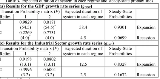
The transition probability matrix, expected duration of system in each regime and steady-state probabilities are given in Table 3. For the entire economy, the probability that expansion will be followed by another year of recession and probability that recession will be followed by expansion another year of are p12 = 0.02 and p21 = 0.22, respectively. It means that expansion regime is highly persistent for the Turkish economy and durations of the expansion and recession periods are approximately 59 and 5 years. These results support the insertion that Turkish economy enters into a recession period every five years.

Table 3. Expected duration of system in each regime and steady-state probabilities (a) Results for the GDP growth rate series (gGDP)

Transition Probability matrix (P)

Rejim 1 2

Expected duration of

system in each regime Steady-State Probabilities 1 0.9829

(54.5) 0.0171 (54.5)* _{58.4 0.9301 Expansion}

2 0.2269

(4.0)* 0.7731 _{(4.0) 4.5 0.0699 Recession}

(c) Results for the Industrial Sector growth rate series (gIND)

Transition Probability matrix (P)

Rejim 1 2

Expected duration of

system in each regime Steady-State Probabilities 1 0.9198 (13.1) 0.0802 (13.1) 12.5 0.8328 Expansion 2 0.3996 (3.2) 0.6004 (3.2) 2.5 0.1672 Recession * _{1 = p + (1 – p)} Since V(1) = V(p) + V(1 – p) then V(p) = V(1 – p)

Durations of the expansion and recession periods for the industrial sector are approximately 13 and 3 years and it means that on average a

recession in the sector lasts about 3 years, whereas an expansion can last for 13 years.

Another advantage of MRS model is to calculate filtered and smoothed probabilities indicating that regimes occurring at time t. The former is computed

given all observations up to time

(

t

−

1

)

observations in the entire sample.

Figure 1 and 2 are prepared to give a better insight to MRS estimates and inferences related to the changes in regime. In each figure, the top panel embodies 5-year (solid line) and 10-year (dashed line) moving average growth rates (grey line) for comparative purposes. The bottom panel plots the filtered (straight line) and smoothed (dashed line) probabilities of being in the expansion regime. The grey horizontal line shows 0.5 probability value.

As can be seen from Figure 1, the number of positive growth rates is more than the number of negative growth rates (especially after 1950’s). This supports our finding that the duration of the expansion regime is 59 years. Moreover, moving averages calculated to see short and long term movements of growth process is higher than µ1 = 4.5% in the 1928-33 periods and under the

% 2 . 4 1 =−

µ _{in the years 1944 and 1945. This is also valid for the 1948-58}

period and the growth rates move between these means.

As is shown in the bottom panel, probabilities of being in the expansion or high growth regime decrease especially in the years 1927, 1932 and the 1941-45 periods. The probability estimates for these years are 0.85, 0.79 and 0.22 respectively. The filtered probabilities of being regime 1 for the year 1941 and the year 1945 are estimated to be 0.26 and 0.006 respectively. The smoothed probabilities for the same years are estimated to be 0.03 and 0.12.

-35.0 -30.0 -25.0 -20.0 -15.0 -10.0 -5.0 0.0 5.0 10.0 15.0 20.0 25.0 30.0 35.0 40.0 45.0 50.0 55.0 19 24 19 27 19 30 19 33 19 36 19 39 19 42 19 45 19 48 19 51 19 54 19 57 19 60 19 63 19 66 19 69 19 72 19 75 19 78 19 81 19 84 19 87 19 90 19 93 19 96 19 99 20 02 20 05 "

Probability of Expansion Regime, Filtered and Smoothed Probabilities (1925–2005) 1932 1927 1941 1945 1980 1989 1994 1999 2001 0.0 0.2 0.5 0.7 1.0 192 5 192 9 193 3 193 7 194 1 194 5 194 9 195 3 195 7 196 1 196 5 196 9 197 3 197 7 198 1 198 5 198 9 199 3 199 7 200 1 200 5

Figure 1. The Hamilton Model fitted to GDP growth rates. The top panel shows the growth rates (grey line) with the 5-year (solid line) and 10-year (dashed line) moving average for comparison. The grey horizontal lines represent the estimated µj. The second panel

plots the filtered (straight line) and smoothed (dashed line) probabilities of being in the expansion regime. The grey horizontal line shows 0.5 probability value.

In this study changes in regime are interpreted according to reference line which is equal to 0.5. The probability estimates indicate that there is one regime switching in the Turkish economy growth process and this change corresponded to the 1941-45 period. Although there is a break in probability

estimates in the crisis years 1994, 1999 and 2001, the probability estimates do not indicate regime changes for these years. In contrast to our expectations the estimates did not indicate a regime changes for the post 1980 period in which industrialization policy has undergone considerable change.

-35.0 -30.0 -25.0 -20.0 -15.0 -10.0 -5.0 0.0 5.0 10.0 15.0 20.0 25.0 30.0 35.0 40.0 45.0 50.0 55.0 1924 1927 1930 1933 1936 1939 1942 1945 1948 1951 1954 1957 1960 1963 1966 1969 1972 1975 1978 1981 1984 1987 1990 1993 1996 1999 2002 2005

Probability of Expansion Regime, Filtered and Smoothed Probabilities (1925–2005) 1971 1961 1950 1941 1937 1929 2000 1949 1936 1945 1988 1994 1980 1999 2001 0.0 0.2 0.5 0.7 1.0 1925 1929 1933 1937 1941 1945 1949 1953 1957 1961 1965 1969 1973 1977 1981 1985 1989 1993 1997 2001 2005 Figure 2. The Hamilton Model fitted to Industrial sector GDP growth rates. The top panel shows the growth rates (grey line) with the 5-year (solid line) and 10-year (dashed line) moving average for comparison. The grey horizontal lines represent the estimated µj.

The second panel plots the filtered (straight line) and smoothed (dashed line) probabilities of being in the expansion regime. The grey horizontal line shows 0.5 probability value.

The top panel in Figure 2 shows the moving average growth rates of the industrial sector. Growth rate values generally fluctuated within the µ1 and µ2 band with the exception of 1932-40, 1954-57 and 1961-69 periods. Moreover growth rate was under this band in the 1943-45 period.

The bottom panel in Figure 2 plots the filtered and smoothed probabilities of industrial sector being in the expansion regime. As can be seen from the figure, in the 1930-35 period probability of being in the expansion regime is quite high. In sharp contrast corresponding values for the year 1936 and 1940-45 period are quite low. The sector moved into an expansion regime 1951-80 period.

The year 1980 is important as policies employed in the industrial sector went under considerable change in this year. Expectedly probability estimates captured this change which because of considerable increase in probability, can be interpreted as a turning point of the business cycles. The policy changes were aimed to transform Turkish economy from import substituting to an export oriented economy and hence 1980 onwards Turkish economy was directly

affected from both global and local changes.

5

from these changes. The probability estimates indicate a break for the years 1994, 1999 and 2001 with respectively probabilities of 0.24, 0.19 and 0.13,

5. Conclusion

In this paper, we analyzed the growth rates under the assumption that in line with the different economic policies applied through the years national income (as GDP) growth rate exhibit a particular structure which might be rendered as regime switching. A similar analysis was undertaken for the industrial sector.

Hamilton, in his seminal paper, described an alternative estimation process to capture the turning point dates for business cycles of U. S. economy. He showed that the NBER chronologies and his chronologies for the business cycles dates were generally fitted.

5 _{As can be seen from the Figure 2, although there is a small decrease in probability value in}

1988, a dramatic change was not observed between the years 1981-94.

The year 1989, in which capital account liberalization policy were implemented, together with 1980 is also important date for the Turkish economy. The Turkish economy has become a much more open economy with these policies. Trade openness and financial openness appeared in the wake of these policies and the two factors affected the growth process of the economy. The relationships between growth process and openness under regime shifts were analyzed by Utkulu and Kahyaoğlu (2005) for the 1990:I-2004:IV period. Another paper by Utkulu and Özdemir (2007) on this subject for the Turkish economy was built upon linear time series analysis. The study analysis whether or not trade liberalization cause a long run economic growth in Turkey.

Estimates of MRS model parameters based on the assumption “there is a regime switching in the mean” are meaningful showing that the dates of expansion and contraction periods in the Turkish economy. It can be interpreted, under this assumption, the periods increasing the filtered or smoothed probabilities in which form a maximum (peak) and the periods decreasing the filtered or smoothed probabilities in which form a minimum (trough) as turning points of business cycles of Turkey. 1932, 1980, 1994, 1999 and 2001 were fond to be the breaking points. These can be interpreted as the turning points of the Turkish economy. However these years do not reflect a regime change in the growth process.

According to estimation results, while the year 1936 and the period of 1941-45 were recession periods, in the industrial sector a dramatic decrease in probabilities was not observed until 1980. As a result 1951-80 period was denoted as expansion regime years. Because of the problems encountered in the early 1990’s and 2000’s 1994-2001 period of can be classified as a recession periods for the sector.

Probability estimates show that development process of the entire economy and development process of the industrial sector are drastically different. Although general growth process covers the growth process of the industrial sector, estimates indicate that it is directly affected by policy changes because of dynamic structure of the sector. Nonetheless, it can be said that Turkey determined his target industrialized economy has to realize these characteristics of the sector determining his policies.

ÖZET

REJİM DEĞİŞİMİ ALTINDA TÜRKİYE EKONOMİSİNİN VE SANAYİ SEKTÖRÜNÜN DEVRESEL HAREKETLERİNİN ANALİZİ

Bu çalışmada Türkiye ekonomisi gayri safi yurtiçi hâsılası (GSYİH) ile sanayi sektörü GSYİH’sının yıllık büyüme hızlarının zaman serisi hareketleri incelenmiştir. Hamilton (1989) çalışmasından hareketle her iki serinin ortalamasında periyodik ve kesikli değişiklikler iki durumlu Markov rejim değişimi modeli aracılığı ile araştırılmıştır. Tahmin sonuçları gerek genel gerekse sektörel büyüme serilerinde ortalamada bir rejim değişikliği konusunda güçlü kanıtlar sunmaktadır. Olasılık tahminleri genel büyüme sürecinde bir, sanayi sektörü büyüme sürecinde beş kez ortalamada bir rejim değişikliği olduğunu göstermektedir.

REFERENCES

BROCK, W. A., W. DECHERT, and J. SCHEİNKMAN, (1987), “A Test for Independence Based on the Correlation Dimension,” Working Paper, University of Wisconsin at Madison, University of Houston and University of Chicago.

BROWN, R. L., J. DURBİN, and J. M. EVANS, (1975), “Techniques for Testing the Constancy of Regression Relationships over Time,” Journal of the Royal Statistical Society, B37, 149-192.

CHOW, G. (1960), “Tests of the Equality between Two Sets of Coefficients in Two Linear Regressions,” Econometrica, 28, 561-605.

ÇINLAR, E. (1975), Introduction to Stochastic Processes, N.J.: Englewood Cliffs.

Devlet İstatistik Enstitüsü, (1973), Türkiye Milli Geliri, Kaynak ve Yöntemler: 1948-1972, Ankara, Devlet İstatistik Enstitüsü Matbaası.

DURLAUF, S., N. (2001), “Manifesto for Growth Econometrics,” Journal of Econometrics, 100, 65-69.

FARLEY, J. U. and M. J. HİNİSH. (1970), “A Test of a Shifting Slope Coefficient in a Linear Model,” Journal of the American Statistical Association, 65, 1321-1329.

GOLDFELD, S. M. and R., E. QUANDT, (1973), “A Markov Model for Switching Regressions,” Journal of Econometrics, 1, 3-16.

GRANGER, C. W. J. (1993), “Strategies for Modelling Nonlinear Time Series Relationships,” The Economic Record, 69, 233-238.

GRAY, S. F. (1995), “An Analysis of Conditional Regime-Switching Models,” Working Paper, Fuqua School of Business, Duke University, Durham, NC.

HAMILTON, J. D. (1989), “A New Approach to the Economic Analysis of Nonstationary Time Series and the Business Cycle,” Econometrica, 57(2), 357-384.

HAMILTON, J. D. (1994), Time Series Analysis, Princeton, N. J: Princeton University Press.

KIM, Chang-Jin and C. R. NELSON, (1999), State-Space Models with Regime Switching: Classical and Gibbs-Sampling Approaches with Applications, Cambridge, Massachusetts: The MIT Press.

Mcleod, A. I. and LI, W. K. (1983), “Diagnostic Checking ARMA Time Series Models Using Squared Residual Autocorrelations,” Journal of Time Series Analysis, 4, 269–273.

ÖZDEMİR, Z.A. and H. Olgun, (2007), “Foreign Exchange Crises, Structural Shifts and Volatility: An Interpretation of the Turkish Case,” The Journal of International Trade and Diplomacy, 1(2), 3-139-158.

QUANDT, R. E. (1972), “A New Approach to Estimating Switching Regressions,” Journal of the American Statistical Association, 55, 324-330.

QUANDT, R. E. (1960), “Tests of the Hypothesis that Linear Regression System Obeys Two Separate Regimes,” Journal of the American Statistical Association, 67, 306-310.

QUANDT, R. E. (1958), “The Estimation of Parameters of A Linear Regression System Obeying Two Separate Regimes,” Journal of the American Statistical Association, 53, 873-880.

RAMSEY, J. B. (1969), “Tests for Specification Error in Classical Linear Least Squares Regressions Analysis,” Journal of Royal Statistical Society, B31, 250-271.

ROSS, S. M. (1983), Stochastic Processes, New York: John Wiley.

STOCK, J. H. (1987), “Measuring Business Cycle Time,” Journal of Political Economy, 95, 1240-1261.

STOCK, J. H. and M. W. WATSON, (1989), “New Indexes of Coincident and Leading Indicators,” in O. J. Blanchard and S. Fischer (Eds.), MBER Macroeconomics Annual, 351-393, Cambridge: MIT Press.

STOCK, J. H. and M. W. WATSON, (1993), “A Procedure for Predicting Recessions with Leading Indicators: Econometric Issues and Recent Experiences,” in J. H. Stock and M. W. Watson (Eds.), Business Cycles, Indicators and Forecasting, 95-156, Chicago: Chicago University Press.

STOCK, J. H. and M. W. WATSON, (1999), “Business Cycle Fluctuations in US Macroeconomic Time Series,” in J. B. Taylor and M. Woodford (eds.), Handbook of Macroeconomics, 3-64, Amsterdam: Elsevier. TAYLOR, H.M. and S. KARLIN, (1984), An Introduction to Stochastic

Türkiye İstatistik Kurumu. (2006), İstatistik Göstergeler: 1923-2005, Ankara: Türkiye İstatistik Kurumu Matbaası.

UTKULU, U. and H. KAHYAOĞLU, (2005), “Ticari ve Finansal Dışa Açıklık Türkiye’de Büyümeyi Nasıl Etkiledi?,” Türkiye Ekonomi Kurumu

Tartışma Metinleri, No: 2005/13, http://www.tek.org.tr/dosyalar/Utkulu-2005.pdf (05/05/2006)

UTKULU, U. and D. ÖZDEMİR, (2004), “Does Trade Liberalization Cause a Long Run Economic Growth in Turkey?,” Economics of Planning, 37, 245-266.