A locally optimal seasonal unit-root test

(1)

Full Terms & Conditions of access and use can be found at

https://www.tandfonline.com/action/journalInformation?journalCode=ubes20

Journal of Business & Economic Statistics

ISSN: 0735-0015 (Print) 1537-2707 (Online) Journal homepage: https://www.tandfonline.com/loi/ubes20

A Locally Optimal Seasonal Unit-Root Test

Mehmet Caner

To cite this article: Mehmet Caner (1998) A Locally Optimal Seasonal Unit-Root Test, Journal of

Business & Economic Statistics, 16:3, 349-356

To link to this article: https://doi.org/10.1080/07350015.1998.10524774

Published online: 02 Jul 2012.

Submit your article to this journal

Article views: 43

(2)

A

Lac;la!iv

CJ

Optima

Seasons!

Unit-

WOO%

Test

h~ahrne:: GAB'.~ER

Sdepeu~nsnt of Economies, Bilkenl Univers~ly, Ankara, Turkey

This article proposes a locally beslt invariant test of the null hypothesis of seasonal stationarity agalnst the alternative of seasonal unit roots at all or individual seasonal frequencies. An asynlprotic distribution theory is derived and the finite-sample properties of the test are examined in a Monte Carla simulation. My test is also compared with the Canova and Hansen test. The proposed test is superior to the Canova and Mansen test in terms of both size and power.

I E Y WORDS: Locally best invariant test; Maximum likelihood estimation; Monte Carlo; Seasonai differencing filter; Seasonal stationarity.

Seasonality in econon~ic time series can be viewed as either deterministic or stoci~~stic. Fitting dummy variables is the usnal way of handling seasonality in a deterministic way To ddiEerenria.te among various patterns of seasonality, statisticai tests are introduced in the literature.

Ey1Yeberg9 Engle, Granger, and Yoo (HEGY) (1990) developed tests of the null hypothesis of a unit root at one or

more seasonal

frequencies against the alternative elf station-

ary scamnality, Their test is ara extension of the unit-root testof Dickey and Fuller

(8939)

from the zero frequency

ro the seasonal frequencies, This test has low pa7vver in finite samples gear unit roots. so it is difficult to reject the false unit-root hypothesis at a single or a set of seasonal frequencies (Canow and Hansen 1995).

In the tests that are developed by Canova and Hansen

(CB)

4,19951, stationary seasonality forms the null hypothesis, The alternative hypothesis is nonstationarity due to seasonal unit roots. They generalized the unit-root test of i<i~viatkowski~ Phillips, Schmidt, and Shin ( O S S ) (1992)

horn the zero frequency to the seasonal frequencies. Their test slatistics are Lagrange mcltiplier (LM) tests that are modified tc include seriajly correlated and hetel-oscedas- tic processes. Only least squares techniq~es are needed in their LM-type test, and autocorrelation is handled by using a nonpararnetric adj~astmeat. Tam and Reinsel (li>95) also conaribuied to this literature by developi~ag tests for moving average

(MA11

seasonal unit roots. Their lest is mainly the extension of the Jaikkonen and Luukkonnen (1993) unit- root test to seasonal frequencies.

In this article, I propose a test procedure in which the null hypothesis of stationary seasonality is testeel against the alternative 3f seasonal nonstationarity. 1 generalize the unit-root test of Zeybouraae and McCabe (1994) fi-om zero frequencg~ BO the seasonal frequency. To test the null hypothesis,

1

propose a locally best l~avariant test that is derived from the framework of King and Hillier (1985). The rest statisrlcs depend on the residuals. which are c;llculated via maxi~num liltellhood and then using least squares. The Barge-sample distribution under the null is the genzeralized

voc

Mises distribution that does not depend on the nuisance para-meters.

a nonparameeric correction. Second, my test statistic is consistent to the order ,"\', whereas the CH test is of order l 7 / z :

where z is the lag truncation parameter. The nonpararnetric adjustment of autocorrelation suggested by Canova and Hansen (1995) fails to give good finite-sample performance when a large autoregressive (AR) component is present in the data. This problem is due to the significant truncztion errors in the finite samples.

The aim of this article is to overcome this problem by introducing a test statistic that accounts for autocorrelation parametrically. A Monte Carlo exercise has been conducted to examine and compare the finite-sample properties of the proposed test with those of the CH test. It is shown that the proposed test has better size arnd power properties than the CH test in en AR type of autocorrelation.

Section 1 introduces the regression model. Section 2

presents the structural and reduced form of the mode:, and a locally best invariant test statistic is also derived for testing unit roots at the seasonal frequencies. The rest of the section develops the asymptotic distribution for this test statistic. Irz

Section 3. a Monte CxBo exercise is conducted, and the size and power properties of the proposed test are compared to those of the CH test. Section 4 concludes the article. Proofs of the theorems are discussed in the Appendix. A

GAUSS

program for calculating test statistics is available on request from me.

1. THE MODEL

A linear time series model with stationary seasonality is considered:

@(L)gt = 11 + S t

+

r t . t = I. 2 , . . .

.

lV.

( I ) In the preceding equation, @ ( L ) = 1 - ol

L

- g2L2 - . . . -

O,LP is a pth-order AR polynomial in the lag operator L

with roots outside the unit circle, yt is real valued, and St

is a real-valued deterministic seasonal process of period s, in which s is a positive even integer and error term el is distributed as rid ( 0 , o,"). The number of observations is LT\f~

If there are

T

years of data,

,V

=

Ts.

Tkere are a wo majol d:Rerences between my test and the

@ 1998 Ameslcat-a Statistical Aseeelaiaosa

CH

test for s e a s o ~ a l stabahty In my test, autocorrelation 1s _Journal_of_Buslwees_Lcl_Economlc_StaUoeEEcs taken ~ n ~ o account in a parametrnc way, but the

CH

test uses duly 1998, voa. 16, No. 3

(3)

Journal of Business & Economic Statistics, July 1998

In this article, because I am interested in anii roots at the seasonal frequencies, 1 require that y, not have a unit root at the zero frequency because it is not very difficult to transform a series with nonstationarity at the zero frequency to a stationary series: various applications of this test will be possible. The autocorrelation in the series is accounted

fmo; by including the lagged terms in yt.

A trigonometric representation is presented for the derer- ministic seasonal pattern

S:

where q = s j 2 (s = 2 fm quarterly data and

.s = 12 for monthly data) and, for j

<

q. f i t =

[ c o s ( ( j / q ) ~ t ) , s i n ( ( j / q ) ~ t ) ] , when j = q. f q t = cos(irt). Ex-

pressing the right side of ( 2 ) in a vector,

These 7 and f t vectors have ( s - 1) elepnei~ts. Substituting ( 3 ) into (11. the regression eqhiatlon is

@ ( L ) y t = p

+

fly

4 e,. t = 1 2 .

Y .

( 5 )

This representation allows sea.sonality to be a cyPicai process. Ah the seasonal frequency j.r;/q, the cylicaP processes are elements of f,. Moreover. f t is a zero-mean process

whenever is a multiple of s. The coe&cients

;,

repre-

sent the effect of each cycle on the deterministic seasonal component

St.

Tsnis cylical formulation of seasonality is common in the time series literature (Miirman 1970, p. 174; Harvey 1989. p. 42).

2. THE

TEST

FOR SEASONAL UNIT ROOTS

2.1 The Structural Model and %he Reduced Form To test whetqer seasonal pattesns are stable or not,

1

need to present a specnfis alternat~ve hypothesis One form of the alternatave hypothes~s 1s to allow a unse root ID - t Thla idea was singgested by Hannan (1970) and rased by Canova and Wanren (1995) and Eeyboume and McCabe

(1994)

The atroctusal model 1s

and

4 0 fixed It as assumed that ut is i~di mean 0, ~nclependent of

et and ft and its covanssnce matrlx are

where

G

is an ( s - 1) x ( s - 1) matrix and 02 is a scalar. The unit roots a: different seasonal frequencies are determined

by

G

matrix. It can be easily seen from

(6)

and (7) that: whenever 0 ; f 6, then there will be seasonal unit roots.

The sir~ctura? model

(6)-(4)

is secoi~d-order eqeaivalent sn momeats ;a the reduced-form model:

where

Ct

is disiributed (0. a:). S ( L ) =

~ g z h

LJ is a seasonal filter, and p' = s ~ .

This Bast term 8 ( L ) is an MA(§ - 1 ) polynomial. The

derivation of

(9)

can be obtained from me on demand. For

the importance s f this representation, the reader can consult Leybourne and McCabe (1994). This reduced form is very similar to the model used by Tarn and Reinsel (1995). Their model did not. however? result in a test that can differentiate between unit roots at various seasonal frequencies and the zero freguencq~.

2.2 The Hypothesis Test

I wish to test whether the seasonal patterns are stable or

not. In other words

1

need to develop a hypothesis so that

I can determine whether a given series has stationary seasonality or not. One such hypothesis is a statioiaary AR(p)

process, against the alternative s f nonstationary seasonality. This can be easily formulaked in terms of the structural model

(6)-(7)

as No : p = 0 against El : p

>

0. where

p = o;,in:. 1 shall examine Ike local departures from the

ntdl hypothesis in the fo9iowing section.

Another task that 1 face is developing a test statistic. From the structural aodel(6)-(7) and using the frameaork of King and Hillier 119851, rhe EocaEly best invariant test statistic for

Ah

: p = 0 Is

where

@,

=

c F = ~

fqei.

6: = &'e/:V is a consistect estimator of a:, and E is an A- x 1 vector or residuals F t .

The residuals

Bt

are obtained via the following procedure: First find the naxirnu.m likelihood estimates of (o) from the fitted model,

where y; = S(L)y, Then construct the series

where

o;

are the maximum likelihood estimates of

nl ob-

tained f r o n

(1

11. Then regress

g,

on an intercept and seasonal olum~mies to obtain &. Even though

1

do not assume the normality of e t , this is necessary for the 'boptirnality"

of the tests.

As pointed out by Saikonnen and Lnnltonnen (1993) and keybourne and McCabe

(19941,

one wants to estimate ql consistently both under the null and the alternatia~e hypothesis in the reduced form, so I use ma:iimui~ likelihood estimation rather than ordinary least squares. Even

(4)

though n~axisnsm li:telahood estimation might have draw- baclcs, they are found to have no effect on the finile-sample

properties of my ".st in the simulations that 1 B-iave con- dncted in the former version of the article (AI-LSP~Y and Ne~.vbold 1380: Gahraith and Zjnde-VValsh

1994).

An alter- ~atlrgme way of estimation is the instrumental-varia.bIe tech- nicpe. But t h ~ s approach did not give good results in this case.

.An

impoi-last p o h t is the structure of

G

matrix. Different specifications of the zlternative hypotheses deperld on the sk-uciv-re ot' G.l&7.'hen the alternative hypothesis is unit roots at a:! seasonal frequencies, then C: must be nonsin;;ular and

?t must be lime a/a;ryirg. If the alternative hypothesis is unit roots at sljecific seaso~al frequencies, then

G

must be block d l a o n a l wilh nonzero elements in only selected blocks and

a snbset of ^it is zime varying,

If the eleernatiire hypothesis is seasonal nonstationarity,

then

1

should have a joint uraie-root test at all seasonal fre- quemies. It was h.rst suggested by Nyblorn (1989) in the Ilikelihood context and later applied to econometric mod-

e3s by Hansen (1990,

1392)

that, when G/az = ( O f ) - l ,

then ;he asymptotic distribution of the test statistic is

easy to evaluale. In the preceding discussion, C!.f is the

Song-run covariance matrix of f i e i (see Canova and Haaasenl 1995).

Becanse et is serially uncorrelated and homosct:dastic,

P

can use the cocsisrenr estimator

-

_lo_study_{she iarge-sample distribution of D, I use the fol-}

d

lowing notation: i denotes convergence in distribution, TITm denotes a vector standard Brownian bridge of dimen- sioaa m., and ?';Ir"(m) is a random ~ a r i a b l e obtained by the following operation:

As was suggested by Canova and Hansen (19951, V;li(m)

~niU be referred to US the generalized von Mises distribution witla rrt df, Criticd values were given in table 1 of Canova and Hansen (1995). The maio theorem of this section is proved in the Appendix.

T!teoism J , In (1). if @ ( L ) is a finite

AR

polynomial in the lag ooeratcr with mots outside the unit circle and if et is iicl, E e i = 0, and E c , ~ = a:

<

x~ then. under LYcl,

Following Section 2.2 and using theorem 3 of Canova and Hansen (1995), 1 have the individual test slatistscs

2 \

D 3 n / q = r x F ; t L b J t . J < Y . (14.1

a,2U2 t=l

and

The individual test stat~stics can be calculated as a by-

product of the joint test. Their asymptotic distributhos is given in Theorem 2.

Theorean 2. Under the conditions in Theorem 1: (1 j for

d d

j

<

q. D,,!,

+

Vii/i(2), and ( 2 ) j = q . D,

-+

VAf(l).

The individual tests supply us with more information about the nature of the seasonal process when there IS ' sea-

sonal nonstationarity in the joins test. Nonstationarity can be caused by she unit roots at the individual seasonal fre-

quencies.

The consistency of the joint and individual tests under

HI

can be obtained via the method described by Eeyboerrne and McCabe (1994). My test is a generalization of the keybourne and McCabe test at zero frequency to the seasonal frequency, whereas the CH Pest is a generalization of the

KPSS test. Both tests have the same limiting distribution. If I analyze the advtintages of the 3 test, first I shorald be-

gin by comparing my test with the

CM

test. The CE test accounts for autocorrelation in a nonparametric fashion, but in finite-samples this can cause problems if the data sarwc- ture contains higher-order terms in the AK polynomial. The

nonpararnetric adjustment then is not able to capture the serial correlation in data. My test focuses on this problem. Autocorrelation is allowed by introducing lagged terms in

y,. This parametric correction is the main advantage of the test and: with a significant AR component in the data. this results in better finite-sample performance. According to Leyboearne and McCabe (19941, the test statistic is consistent at a rate O,(N) under

MI,

but in the MPSS teest this rate is U,(Ai/z) ( z is the bandwidth parameter in KPSS and CR tests). These rates also apply to my test statistic and the

CH

test statistic under H I . Therefore, I expect my test's power to be better.

3. MONTE CARLO STUDY

To examine the size and power properties of the proposed test statistics, a Monte Carlo exercise is conducted. Two quarterly models are considered. The first model is

2

@(E)yt = p

+

JL,/,-/,t

+

e t , et

-

lY(0. l), (16)

1=1

and

where70 = [[i,l,l],-/t = (yLb.-y~t)i, a n d o

<

6 5

1. 72i is a

(5)

352 Journal of Business & Economic Statistics, July 1998

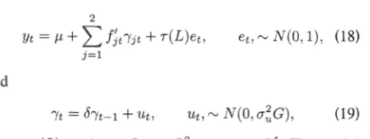
AR(p) process. The second model is given by

and

where

T(L)

= L

+

r l L

+

raL2

+

. .

. T&&. The model ("a)-(19) ensures a fair comparison between the D test and the CH test because my test captures an AW(p) type of autocorrelation. In calculating the size of the tests,

1

explore the more empirically relevant case of 0

<

6

<

1 and U: f 0.

For both models, three different data-generating processes (DGP's) are used under the alternative hypothesis-

and

Under DGP I 9 there is a unit root at the 7i- frequency as

long as D:

#

0. The D, test is designed for this specifi-

cation. There is a pair of complex conjugate roots at the

r;/2 frequency itnder DGP2 when D: f 0. Similarly, when

B: = 0 under DGP 4 there are no unit roots, but there are unit roots at all seasonal frequencies if u,', f 0. One important fact to note is that the covariance structure implied by

G is different from the one that is used to construct the D and

D,;,

test statistics.

In the simulations, the order of the AR polynomial p and the order of the MA polynomial il are

P

and 2. Both the AW

parameters of (1 6)-(17) and the MA parameters of (1 8)-(19)

are chosen carefully to understand the eRect of autocorre- Iation on the test statistics that are proposed in this article.

1 set b = .X. The signal-to-noise ratio p = 0:/0,2 takes the value of .05.6 vary the sample size among ilT = 50.100.200.

I have 1,000 independent realizations for each DGP and parameter configuration. The test statistics are calculated for unit roots at all, T~ and n/2 seasonal frequencies. Robust-

ness issues are explored in Subsec~ion 3.3.

My test's finite-sample properties are compared to those of the CW tests (with and without one lag of the dependent vanable included). Hylleberg (1995) showed that the

CH

test with one lag bas iow power. Because 1 analyze various data structures. however, ]I want to include that test in my study also. The underlying model of the

CH

test is the same as my model (16)-(17) and (20)-(22), but they assume p = 0 or p = 1. Because they also assume an a-mixing process for

Tabe 1. Size and Power Gompsrison Between the CH and D tests: AR Model

B CHo CHi DGP SS J

-

~ i 2 J 7~ 7;/2 J 7i ~ / 2 Size Size Size BGP3 DBP3 BGP3 DGP2 BGP2 DGP2 DGP1 DGPl BGP1 Sine Size Size BGP3 DGP3 BGP3 BGP2 BGP2 DGP2 DGPl DGPI DGP1

NOTE. In both AR pararnetertzattons for the stze part. 7 , = .Byt-, i u; For the power part of fhe program, =

-,-,

+ ut SS IS the sample slze. D. CHa, and CHI are the D and the CH tests with no lags and one lag. respectively J, 7 , and 7i!2 are the tests at all. semiannual. and annual seasonal frequencies, respectively The DGP column shows the size and :he power of the tests (DGP3. DGPP, DGP;).

(6)

e,, their estilcnates of long-run covariance matrices

hf

and for p = P and p = 0, respectively, depend on the choice s f the kernel and she lag truncation number z. In this study the 3artletn kernel is used and, following Andrews (1991),

z = 3.4; 6 is sclected for ;'1 = 50; 100.200, respectively.

One important point about mgl test is the choice of p, the number of lags in y,. The D tests ape carried out with lag lengths chosen by the Akailte information criterion (AIC) and the Bayesian information criteriori

(BlC).

The results of the exercise zre presected in Tables 1 and

2. The percentage of rejection of the null is given at the 5% significance level. Because the size of the D and CH tests that are calculated in Tables 1 and 2 vary consicierably, I

calculizse she size-adjusted power, In the tables, the power

of the tests are size-adjusted power. The critical values for calceulati.ng these can be ohpained from me on demand.

There are three Monte CarPo studies than compare the rel- ative performance of the tests for seasonal stability. One is by Hyllebesg (1995) in which the WEGY tests are contrasted with the CH tests. Ghysels, Lee, and Noh (1 994) compared

"re performance of the HBGY test with the Dlickely, Hasza, and Fnler (1984) tests. Canova and Hansen (1995) contrasted the

CH

tests with

HEGY

tests, but the DGB is different from the Monte Carlo study

d

Hylleberg (1995).

3.1 Size and Power sf t h e Test: AR(p) Process

Ba t h ~ s section the size and power properties of the D test are compared with the

CH

test under the model (16)-(17). When analyzing the s u e of the tests in Table I, b 1s selected

to be

.a

because this value corresponds to a "near" seasonal unit root. In calculating the power of the tests in Tables I

and 2, I set b = 1.

In Table I , it is easy to see that the size of my tests is slightly above the nominal size of 5% in most of the cases. The CH tests have large size distortions for JaR(2) parameterization, however. For example, for N = 200 in an AW(2) framework, the size of the goint D test is 14%.

whereas the joint

CM

tests reject the true null in 41-50% of the trials.

The D tests have good power under different alternatives. For 1V = 100, the power of the joint test is 84% when there are seasonal unit roots present at the a/2 frequency

(DGP2). For AT = 200, In an AR(2) process, the power of the joint test is 85% when there is a seasonal unit root at the T frequency (DGPI).

The CH tests ha.ve mixed results under an AR structure. For

i

Y

= 100, in an AR(1) process the

joint

test has

Q&

79% power against DGP2. The CH tests with one lag sf the dependent variable (CHI in Tables 1-2) perform quite poorly in an AR(1) structure. The power is near the nominal size of the tests. Both

CH

tests also have trouble in an AR(2) structure when only a seasonal unit root at the x frequency is present (DGPB). For N = 200, the joint tests have 56%

power under DGBH.

Overall, the

CH

tests do not perform well near seasonal unit roots. They suffer from size distortion. On the other hand, the proposed tests have good size and power, The

CH

tests performed well in the Monte Carlo study s f Canova

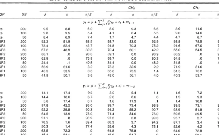
Table 2. Comparison of SL?e and Power: The CH and D tests in an IWA Model

B - CHo CHr DGP SS J T x / 2 J K 7i/2 J 7i TIP S ~ z e S ~ z e Size D G P 3 D G P 3 D G P 3 D G P 2 D G F 2 D G P 2 D G P I D G P I DGP1 S ~ z e S ~ z e S l z e D G P 3 D G P 3 B G P 3 DGP2 B G P 2 DGP2 D G P ? D G P I DGPI

(7)

Journal of Business & Economic Statistics. July 1998

and Hansen (1995) because of the structure of the DGP

that they used. Their simulated models are not "near" seasonal unit roots at various frequencies, so it is difticult to determine the size in their study appropriately. In our case the simulated models correspond to an "almost" seasonal nonstalionary case.

3.2 Size and Power of the Test: MA(1) Process

In this section the DGP is (18)-(191, which is the case with MA(Y) errors. This bind of setup provides a neutral ground for comparing our tests with the CH tests. Two types of MA processes are explored in Table 2. First I use

Then the following MA(2) process is analyzed:

I set 6 = .8. T = .&, and a: = .05. Using the AIC and

BIC, the optimal AR lag length p turned out to be 3, 5, and 6, f o r I V = 50,100,200, respectively.

Table 2 shows that the proposed D tests have good size. The test at the n/2 frequency performs well even in the small samples. For example, for

N

= 50 in an MA(1) process, the size is 7%. Even though the test at the n frequency performs well in an MA(1) model, however, the size rises above the nominal level and is around 9-21% in an MA(2)

setup.

The CH tests also have good size properties. For example, the size of the joint CH test with no lags of the dependent variable kCHo) is 2-1196. The sizes of both tests do not seem to be affected by the sample size.

Both the D and CH tests have good power under different alternatives. Note. however, that the asymptotic rejection frequency of the

D

tests is better than that of the CH tests. These results were given by Caner (1994).

tecting the presence of seasonal unit roots in time series models. The null hypothesis of the proposed test is seasonal stationarity. whereas the seasonal unit-root hypothesis forms the alternative. The derived asymptotic distribution is nonstandard and covers serially correlated processes. My test is similar to the CH test for seasonal stability. The main difference between the two arises from handling autocorrelation under the respective null and alternative hypotheses.

My test has a parametric correction, but the CH test has a nonparametric adjustment for autocorrelation. According to my simulations the CM test suffers from size distortion in an AR model, whereas the proposed test has good size and power. Moreover, even with different autocorrelation structures and data-generating processes, the proposed tests have good finite-sample properties.

ACKNOWLEDGMENTS

1 thank Bruce Hansen for helpful advice, encouragement, and comments. 1 also thank Bent Sorensen for letting me use his UNIX workstation and the editor, associate editor. and two anonymous referees whose comments improved the article considerably.

APPENDIX: DERIVATION OF THEOREMS Before proving the theorems, I need to prove a lemma and introduce some notation. Let

+

denote weak convergence on [O, 11 with respect to the uniform metric, let [.] denote integer part, and !et

3

denote convergence in probability.

kemnza I .

where B(rj is a three-dimensional Brownian motion with covariance matrix

flf

.

Proof of Lemma 1. From the structural model under the null hypotheses:

1

obtain

3.3 The Robustness Experiments

The results are robust to overfitting of the AR poiyno- snial, correlatedness of ut and e,, and overdifferencing of

g t Specifically, when 1 tried fitting up to SIX lags for AR(1) and AR(2) models. there were no significant changes in the power and size of the test. The fimte-sample properties of the test were also analyzed by using vanous 02's and 6's. The size and the power of the test were not affected by the changes in a:. Smaller S and AR coefficients resulted in better size properties for my test. Monte Carlo designs with longer AR polynomals such as 3 and 4 were tried, gen- eratlng results that were very similar to the case of AR(2) design in Table 1.

4. CONCLUSION

From the first-order conditions, I know that l i i ~ ~ ; : , ftBt = 0, so I have

(8)

A

In this expression each term will be examined in detail. Noav, observa that, from the first term on the right side of

i"a.31,

In

(A.41,

af 'ST] I S a mul'iple of s. then ( k . 4 ) 1s O because f t

i s a zero-meaa process.

IS

[ l v r ] is not a multiple c ~ f s when

i m, (A.4) converges to 0,

ar~d., from Potscher (19919, [' -

f i )

is o,(l).

The same procedure applies to the second term on the right side of (A.3) as well.

For the third term, under the null hypothesis g t - ~ is an

AR(p) process. Folowing from the invariance principle for

linear processes (PtilPips and Solo 1992),

converges weakly and is Op(1j. Then, horn Potscher

119911,

1 know tha: (ol - dl ) is o,(!), so

Finally, invoking the functional central limit theorem (Billingsley

19681,

where B(T) 1s a vector Brownian motion with covariance

matrix Q f , Combining BA.3,

(A.61,

and bA.'7), 1 obtain

PI-sof of Theorem I . From Lemma 1 and applying the continuous mapping theorem, I obtain

Proofof Theorem 2. This theorem is proved in a manner similar to the proof of Theorem 1.

[Received September 1996. Revised May 1997.1

REFERENCES

Andrews, D. ( 1 991). "Heteroskedasticity and Autocorrelation Consistent Covariance Matrix Estimation," Ecoizometrica. 59. 817-8558,

Ansley, C. F., and Newboid, P. (1980). "Finite Sample Properties of Esti- mators for Autoregressive Moving Average Models." Journal of Ecoizo- metrics, 13, 159-183.

Biilingsley, P (1968), Convergence of Probability ~Meas~~res, New VorEc: IViley.

Caner, M. (19961, "A Locally Opiimal Seasonal Unit Root Test," working paper. Koc University, Dept. of Economics.

Canova, E. and Hansen, B. E. (19951, "Are Seasonal Patterns Constant Over Time? A Test for Seasonal Stability," Jo~irnal ofBusiizess & Eco- nomic Smtistics: 13, 237-252.

Dickey, D., and Fuller, W. (1979), "Distribution of the Estimators for Au- toregressive Time Series With a Unit Root," jhzlrnal of the Atnericaiz Statistical As~ociurioiz, 84. 4 2 7 4 3 1 .

Dickey, D., Hasza, D., and Fuller, W. (1984), "Testing for Unit Roots in Seasonal Time Series," Journal of the Anlericun Statistical Associaiion,

79, 355-367.

Calbraith, J. W., and Zinde-Walsh, V. (1994), "A Simple Noniterative Es- timator for Moving A\erage Models;' Biometrika. 81. 143-1555, Ghysels, E., Lee. B.. and Noh, J. (1994), "Testing for Unit Roots in Sea-

sonal Time Series: Some Theoretical Extension and a Monte Carlo In- vestigation," Jourizal of Econometrics. 62, 41 5 4 4 2 .

Hannan, E. J. (1970). Multiple Time Sel-ies, S e v ~ York: Wiiey.

Hansen, B. E. (19901, "Lagrange Multipler Tests for Parameter Instability in Nonlinear Models," working paper, University of Rochester, Dept. of Economics.

-- (i992), "Testing for Parameter Instability in Linear Models," Jour- ;la1 of Policy Modeling, 14, 517-533.

Harvey, A. C. (1989): Forecarting Stv~tctural Time Series Models and tlze Kalinarz Filter. Cambridge, C.K.: Cambridge University Press. Hylleberg, S. (1995), "Tests for Seasonal Unit Roots: A Comparative

Study:' Jcz~rlial of Ecorzomet~ics. 69, 5-25.

Hylleberg. S., Engle. W., Grangcr, C., and Yoo, S. (1990), "Seasonal Pnte- gration and Cointegration." Jorrrnal of Ecunonzetrics, 44, 215-238.

(9)

356 Journal of Business & Economic Statistics, July 1998

King. ht. L., and Hillier, 6 . H. (19851, "Locally Best Invariant Tests of the Error Covariance Matrix of the Linear Regressiol~ Model," Jorrnrnl of the Royal Statistical Society, Ser. B, 47, 98-102.

I<wiatkoiislri, D., Phillips, P. C. B.. Schmidt, P., and Shin, Y (1992). "Test- ing the Wull Hypothesis of Stationarity Against the Alternative of a Unit Root: How Sure Are We That Economic Time Series Have a Unit Root?"

hurnal of Ecoizonzetric.r, 44, 159-178.

Leybourne, S. J., and McCabe, B . P. M. (1994), "A Consistent Test for A Unit Root," Jocrrnal of Business & Economic Statistics, 12. 157-167. Nyblom, J. (1989), "Testing for the Constancy of Parameters Over Time,"

.foz,rnaZ of the American Statistical Associution, 84, 223-230.

Phillips, P. C. B., and Solo, V. (1992). "Aspmptotics for Linear Processes."

The Atzrzals of Statistics. 20. 971-1001.

Poischer, B. M. (1991), "Non-invertibility and Pseudo-Maximum Likeli- hood Estimation of Mis-specified ARMA models," Econometric Theoiy,

7 , 4 3 5 4 4 9 .

Saikkonen, P.. and Luukiconen, R. (1993), "Testing for a Moving Aver- age Unit Root in Autoregressive Integrated Moving Average Models."

Journal of the American Statistical P.ssociation, 88, 596-601. Tam, W., and Reinsel, C. (1995). "Tests for Seasonal Moving Average

Unit Root in ARIMA Models.'' working paper, University of Wisconsin. Madison, Dept. of Statistics.