a dissertation submitted to the department of mathematics
and the institute of engineering and science of bilkent university
in partial fulfillment of the requirements for the degree of
doctor of philosophy
By
Natalya Zheltukhina July, 2002
Prof. Dr. Iossif V. Ostrovskii(Supervisor)
I certify that I have read this thesis and that in my opinion it is fully adequate, in scope and in quality, as a dissertation for the degree of doctor of philosophy.
Asst. Prof. Dr. C. Yal¸cın Yıldırım (Former Supervisor)
I certify that I have read this thesis and that in my opinion it is fully adequate, in scope and in quality, as a dissertation for the degree of doctor of philosophy.
Assoc. Prof. Dr. Turgay Kaptanoˇglu
Prof. Dr. Mefharet Kocatepe
I certify that I have read this thesis and that in my opinion it is fully adequate, in scope and in quality, as a dissertation for the degree of doctor of philosophy.
Assoc. Prof. Dr. Sinan Sert¨oz
Approved for the Institute of Engineering and Science:
Prof. Dr. Mehmet Baray Director of the Institute
ON SECTIONS AND TAILS OF POWER SERIES
Natalya ZheltukhinaPh.D. in Mathematics
Supervisor: Prof. Dr. Iossif V. Ostrovskii July, 2002
The thesis is devoted to the study of connections between properties of a power series and properties of its sections and tails.
Power series having sections or tails with multiply positive coefficients are considered and their growth estimates are obtained. Our results strengthen and supplement previous results in this direction, in particular, the well-known P´olya theorem on power series with sections having only negative zeros.
The asymptotic zero distribution of linear combinations of sections and tails of the Mittag-Leffler function E1/ρ of order ρ > 1 is studied. Our results generalize
and supplement previous results in this direction, in particular, the well-known Szeg¨o result on the linear combinations of sections and tails of the exponential function and the A Edrei, E.B. Saff and R.S. Varga results on sections of E1/ρ.
Keywords: Laurent series, Mittag-Leffler functions, m-times positive sequence,
power series, sections, tails, zero distribution.
KUVVET SER˙ILER˙IN˙IN KISM˙I TOPLAMLARI VE
KUYRUKLARI
UZER˙INE
¨
Natalya Zheltukhina Matematik B¨ol¨um¨u, Doktora
Tez Y¨oneticisi: Prof. Dr. Iossif V. Ostrovskii Temmuz, 2002
Bu tez kuvvet serilerinin kısmi toplamlarının ve kuyruklarının ¨ozellikleri arasındaki ba˘glantıları ¸calı¸smaya adanmı¸stır.
Kuvvet serilerinin kısmi toplamlarının ya da kuyruklarının ¸coklu pozitif kat-sayılı olanları ele alınmı¸s ve bunların artı¸s hızı tahmin edilmi¸stir. Sonu¸clarımız bu alanda daha ¨onceden bulunmu¸s sonu¸cları, ¨ozellikle kuvvet serilerinin kısmi toplamları negatif katsayılı olanları ¨uzerine olan ¨unl¨u P´olya teoremini, geni¸sletmekte ve tamamlamaktadır.
Ayrıca, derecesi birden b¨uy¨uk olan Mittag-Leffler fonksiyonlarının kısmi toplamlarının lineer kombinasyonlarının sıfırlarının asimptotik da˘gılımı da ¸calı¸sılmı¸stır. Sonu¸clarımız bu alanda da daha ¨onceki sonu¸cları, ¨ozellikle de Szeg¨o’n¨un ¨ustel fonksiyonun kısmi toplamlarının lineer kombinasyonları ¨uzerine ve A. Edrei, E. B. Saff ile R. S. Varga’nın Mittag-Leffler fonksiyonlarının kısmi toplamları ¨uzerine olanlarını, genelle¸stirmekte ve tamamlamaktadır.
Anahtar s¨ozc¨ukler : Laurent serisi, Mittag-Leffler fonksiyonları, m-katlı pozitif
dizi, kuvvet serisi, kısmi toplamlar, kuyruklar, sıfır da˘gılımı.
I would like to express my deep gratitude to Prof. C. Y. Yıldırım for his constant and continual support, valuable suggestions and discussions.
I take great pleasure in expressing my sincere gratitude to Prof. I. V. Ostro-vskii. Over many years he provided me with generous support and much helpful guidance.
I wish to thank my husband Kostyantyn Zheltukhin and our daughter Anna for their being part of a supporting family.
Finally, I would like to thank the Department of Mathematics of Bilkent Uni-versity for excellent working conditions and creative and warm atmosphere.
1 Introduction 3
2 Statement of results 7
2.1 Power series with multiply positive coefficients . . . 7 2.2 Laurent series with multiply positive coefficients . . . 14 2.3 The distribution of the zeros of sections and tails of the Mittag–
Leffler functions . . . 19
3 Preliminaries 29
3.1 One-sided multiply positive sequences . . . 29 3.1.1 One-sided sequences having sections with multiply positive
terms . . . 33 3.1.2 One-sided sequences having tails with multiply positive terms 35 3.2 Two-sided multiply positive sequences . . . 37 3.3 Power series with sections from P F∞ . . . 38
3.4 Some asymptotic relations for Mittag-Leffler functions . . . 39
4 Power series of sections with m-times positive coefficients 43 4.1 The lower bound for d(P4) . . . 44
4.2 The upper bound for d(P4) . . . 49
5 Power series having tails with m-times positive coefficients 57 5.1 The lower bound for d(R4) . . . 58
5.2 The upper bound for d(R4) . . . 60
6 Laurent series with m-times positive coefficients 64 6.1 Connection between two-sided and one-sided multiply positive
se-quences . . . 66 6.2 Parametric representation of sequences from ˜Q3. Growth
esti-mates . . . 71
7 Zeros of sections and tails of Mittag-Leffler function 75 7.1 Asymptotic expressions for In(Rnz; λ, E1/ρ) . . . 79
7.2 Zero-free regions of In(Rnz; λ, E1/ρ) . . . 84
7.3 The asymptotic behavior of In(Rnz; λ, E1/ρ) in the neighborhood
Introduction
Let f (z) = ∞ X k=0 akzk, a0 > 0, (1.1)be a formal power series. Denote by R(f ) its radius of convergence, and by
sn(z; f ) = n
X
k=0
akzk, n = 0, 1, 2, . . . , (1.2)
its sections. For R(f ) > 0, denote by
tn(z; f ) =
∞
X
k=n
akzk, n = 0, 1, 2, . . . , (1.3) the tails of the series (1.1), and set
M(r, f ) = max
|z|=r|f (z)|, 0 < r < R(f ).
The study of the distribution of zeros of sn(z, f ) was started at the end of
19th century. The first important result concerning the distribution of zeros was a work of A. Hurwitz (see [18]). Later on, in the first half of 20th century, deep and general results revealing connections among the asymptotic (as n → ∞) behavior of zeros of sn(z, f ), the radius of convergence R(f ) of (1.1) and the
growth of function f in terms of M(r, f ) were obtained in works of G. P´olya [29],
R. Jentzsch [19], G. Szeg¨o [35], P.C. Rosenbloom [32], F. Carlson [6], A. Dvoretzky [10] and others. For some widely applicable concrete entire functions (such as the exponential function, the trigonometric functions and some others) elegant and sharp asymptotics (as n → ∞) for zeros of sn(z, f ) were obtained by G. Szeg¨o [36],
J. Dieudonn´e [8] and P.C. Rosenbloom [32]. For a review of these results, as well as a detailed bibliography, the reader may consult the thesis of P.C. Rosenbloom [32].
During the second half of 20th century in works of T. Ganelius [15], [16], J.D. Buckholtz [3], [4], [5], J. Korevaar [21], A. Edrei [13] and other mathemati-cians some important unsettled problems have been solved and new general phe-nomena have been discovered. Obtained earlier by G. Szeg¨o [36] and J. Dieudonn´e [8] asymptotics for the zeros of sn(z, f ) of some concrete entire functions have
been considerably improved by J.D. Buckholtz [2], A.J. Carpenter, R.S. Varga, J. Waldvogel [7], D.J. Newman, T.J. Rivlin [22] and others. In the work of A. Edrei, E.B. Saff and R.S. Varga [12] these asymptotics were extended to the Mittag-Leffler functions which generalize the exponential function.
Apparently, the first study of the zero distribution of tails tn(z, f ) has been
done by G. Szeg¨o in [36] where even a more general problem of the asymptotic distribution of the zeros of the linear combination
In(z, λ, ez) = (1 − λ)sn(z, ez) − λtn(z, ez) (1.4)
for any λ ∈ C was considered. Evidently, In(z, 0, ez) = sn(z, ez) and In(z, 1, ez) = tn(z, ez).
In the general case, the study of the distribution of the zeros of tn(z, f ) of an arbitrary power series (1.1) with a positive radius of convergence was initiated by
M. Pommiez [31] in 1960. In 1970s, J.D. Buckholtz and J.K. Shaw [5] continued this investigation and obtained complete solutions for some problems related to
the distribution of the zeros of sections sn(z, f ) and tails tn(z, f ). In 1990s new
results on the distribution of the zeros of tn(z, ez) were obtained by C.Y. Yıldırım
[37], [38], [39], who needed them for the evaluation of some terms that came up in certain mean-value estimate related to the ζ-function. Recently, I.V. Ostrovskii [23], [24] has found a new phenomenon on the distribution of the zeros of tails
tn(z, f ) in terms of the arguments of the zeros. A survey of investigations prior to 1997 on several aspects of the distribution of zeros of sections and tails is given by I.V. Ostrovskii in [25].
The present thesis is devoted to the study of some open problems concerning the asymptotic distribution of the zeros of sections sn(z, f ) and tails tn(z, f ).
In a previous work of I.V. Ostrovskii and the author [26] a new generalization of P´olya’s Theorem [29] on formal power series whose sections have only negative zeros was found. This generalization was achieved by introducing some classes
Pk of power series with multiply positive (in the sense of M. Fekete) coefficients.
These classes form a decreasing sequence P1 ⊃ P2 ⊃ . . .. Moreover the class
P∞ := ∩∞k=1Pkis exactly the class of power series that appears in P´olya’s Theorem.
In [26] it was shown that the statement of P´olya’s Theorem remains in force for the much larger than P∞ class P3, and hence for all the smaller classes Pk, k ≥ 4 (it fails for the classes P1 and P2 as can be seen on simple examples).
In [26] a sharp growth estimate for functions of P3 has been obtained. This
estimate certainly holds in all the classes Pk, k ≥ 4. However, it was not known
before whether this estimate is sharp in Pk, k ≥ 4, or not. In Chapter 4, we
give a negative answer to this problem and find an improvement of the estimate obtained in [26] for the classes Pk, k ≥ 4.
In another work of I.V. Ostrovskii and the author [28], analogous results for tails tn(z, f ) have been given. Similar to Pk, classes Qk of power series with
multiply positive coefficients have been considered in [28]. The classes Qk also
form a decreasing sequence Q1 ⊃ Q2 ⊃ . . .. Results obtained in [28] are sharp in
Q3. However, it was unknown before whether they are sharp in the classes Qk, k ≥ 4, or not. In Chapter 5, we show that a growth estimate obtained in [28] is
not sharp in Qk, k ≥ 4, and improve it for Qk, k ≥ 4.
A Laurent series can be viewed as a generalization of a power series. To the best of our knowledge, the distribution of the zeros of sections of Laurent series has not been studied before. In Chapter 6, we obtain a generalization of results of [26] to Laurent series.
In the work of A. Edrei, E.B. Saff and R.S. Varga [12], the distribution of the zeros of sections sn(z, f ) of Mittag-Leffler functions
E1/ρ(z) = ∞ X k=0 zk Γ³1 + k ρ ´, ρ > 1,
was studied. When ρ = 1, the Mittag-Leffler function coincides with ez. In [12],
the authors generalized some results of [36] to the class of Mittag-Leffler functions. However, as mentioned before, in [36], the zeros not only of sections sn(z, ez) but
also, more generally, of the linear combinations (1.4) have been considered. The question arises about such a generalization of results of [12] that contains the complete result of G. Szeg¨o on the linear combinations (1.4). In Chapter 7 we obtain such a generalization.
The results of this thesis have been accepted [40], [41] and submitted [42] for publication.
Statement of results
2.1
Power series with multiply positive coefficients
In 1913, G. P´olya proved the following theorem.
Theorem A ([29]). If, for all sufficiently large n, sections (1.2) have real
negative zeros only, then R(f ) = ∞ and
log M(r, f ) = O((log r)2). (2.1)
This result shows that restrictions on argument of the zero distribution of sections can imply a rather serious growth restriction on the original power se-ries. Since then, formal power series with restrictions on zeros of their sections have been deeply investigated by several mathematicians. The most far reaching generalization of P´olya’s result was obtained by T. Ganelius in 1963.
Theorem B ([16]). Assume that there exist α > 0 and a sequence of real numbers
{γn}∞n=1 such that sections (1.2), for all sufficiently large n, do not vanish in the
angle
{z : γn< arg z < γn+ α}.
Then R(f ) = ∞ and (2.1) holds.
In the paper by I.V. Ostrovskii and the author [26], a generalization of The-orem A whose character is quite different from that of TheThe-orem B has been obtained. It is based on concept of multiple positivity introduced by M. Fekete in 1912.
Let R∞ be the set of all sequences of real numbers, and sequences a = {an}∞n=−∞ and {bn}∞n=−∞ belong to R∞. Let
a ∗ b = {(a0 · bk+ a1· bk−1+ . . . + ak· b0)}∞k=0
be the convolution of the sequences a and b. Denote by ν[a] the number of changes of sign in the sequence a.
Definition 1. A sequence a is called m-times positive, m ∈ N, if for all b ∈ R∞
satisfying ν[b] ≤ m − 1, we have ν[a ∗ b] ≤ ν[b]. A sequence a is called ∞-times
(or totally) positive if ν[a ∗ b] ≤ ν[b] for all b ∈ R∞.
There is an equivalent but more convenient definition of multiply positive sequences (see [20]), even though its formulation is somewhat complicated: Definition 2. A sequence a = {ak}∞k=0 of real numbers is said to be m- times positive for m ∈ N ∪ {∞} if all minors of orders less than m + 1 of the infinite
matrix a0 a1 a2 a3 . . . 0 a0 a1 a2 . . . 0 0 a0 a1 . . . . . . . . . . are non-negative.
Multiply positive sequences were introduced by M. Fekete [14] for the study of zeros of real polynomials and entire functions. Since then such sequences have been studied by several mathematicians and have found many applications (see, e.g. [1], [20]).
Denote by P Fm, m ∈ N ∪ ∞, the set of all m-times positive sequences. If
series (1.1) is a generating function of such a sequence, we shall also write f ∈
P Fm. Evidently,
P F1 ⊃ P F2 ⊃ . . . ⊃ P F∞.
Clearly, the class P F1 consists of all the sequences {ak}∞k=0with positive terms.
It is easy to see that the class P F2 consists of all the sequences of the form
an = exp{−ψ(n)}, n = 0, 1, 2, . . . ,
where ψ : N ∪ {0} → (−∞, +∞], ψ(0) < ∞, is a convex function. The problem of the description of the classes P Fr for 3 ≤ r < ∞ is at present far from
being solved. Nevertheless, the smallest class P F∞ (contained in all P Fm, m ∈
N ∪ {∞}) had been completely described by M. Aissen, A. Edrei, I.J. Shoenberg and A. Whitney.
Theorem C([20], p.412). A function f (z) belongs to P F∞ if and only if f (z) = C exp(qz) ∞ Y i=1 (1 + αiz) (1 − βiz) , (2.2) where C > 0; q, αi, βi ≥ 0, ∞ X i=1 (αi+ βi) < ∞. (2.3)
Theorem C yields that an entire function (1.1) of genus 0 has purely negative zeros if and only if the sequence {ak}∞k=0 is totally positive. Applying this to
of the truncated sequence
{ak}nk=0 = {a0, a1, . . . , an, 0, 0, . . .}.
Thus the condition of P´olya’s Theorem A is equivalent to total positivity of the truncated sequences {ak}nk=0 for all sufficiently large n.
Denote by Pm, m ∈ N ∪ {∞}, the class of all power series (1.1) such that
the truncated sequences {ak}nk=0 are m-times positive for all sufficiently large n.
Evidently,
P1 ⊃ P2 ⊃ P3 ⊃ . . . ⊃ P∞.
In [26] the following question was considered. Does the assertion of Theorem A remain in force if we replace total positivity of the truncated sequences {ak}n
k=0
by a weaker condition of their m-times positivity for some m < ∞? It is easy to see that the answer is negative for m = 1 and m = 2. For example, if ak = 1 for
any k = 0, 1, 2, . . ., all the truncated sequences {ak}nk=0 are 2-times positive, but
the series (1.1) does not converge in the whole complex plane C. It was proved in [26] that the situation changes if m ≥ 3.
Theorem D([26]). If a formal power series (1.1) belongs to Pm for some m ≥ 3, then it converges in the whole complex plane and its sum f (z) is an entire function of order 0. Moreover, lim sup r→∞ log M(r, f ) (log r)2 ≤ 1 2 log c, c = 1 +√5 2 = 1.613 . . . (2.4)
The estimate (2.4) cannot be improved for f ∈ P3.
The question arises whether the estimate (2.4) is unimprovable for m ≥ 4. It will be shown in Chapter 3 that following P´olya’s own proof of Theorem A, one can improve the estimate (2.1) for functions satisfying the condition of The-orem A (which is equivalent to the condition f ∈ P∞). More precisely, the
following theorem holds.
Theorem E. If, for all sufficiently large n, sections (1.2) have real negative
zeros only (or, equivalently, f ∈ P∞), then the bound (2.4) can be improved in the following way:
lim sup r→∞ log M(r, f ) (log r)2 ≤ 1 2 log 2. (2.5)
As far as we know, the question whether P´olya’s estimate (2.5) is sharp has not yet been settled. In [30] ( Part V., Problem 176), an example was con-structed showing that log 2 cannot be replaced by a constant greater than log 4. O. M. Katkova and A. M. Vishnyakova kindly informed me that, by modifying this example, they showed that log 2 cannot be replaced by a constant greater than log(3.5).
In the present work we show that an estimate better than (2.5) already holds in the class P4 which is much larger than P∞. Our first result is the following
theorem.
Theorem 1 . If f ∈ Pm, m ≥ 4, then the bound (2.4) can be improved in the following way: lim sup r→∞ log M(r, f ) (log r)2 ≤ 1 2 log d(P4) , (2.6)
where the constant d(P4) is independent of f and
2.016 ≤ d(P4) ≤ 2.087.
One may approach the problem of finding the sharp estimate in Theorem E by obtaining the sharp growth estimates for functions from Pm, m ≥ 4. This
problem remains open for any m ≥ 4.
Note that for m < ∞ there is also a relation between m-times positivity of the sequence {ak}n
a less strict one than for m = ∞. I. J. Schoenberg ( [33], pp.397, 415 ) proved: (i) the necessary condition for {ak}n
k=0 to be m-times positive is the non-vanishing
of (1.2) in the angle {z : | arg z| ≤ (πm)/(m + n − 1)}, (ii) the sufficient condition is its non-vanishing in the larger angle {z : | arg z| ≤ (πm)/(m + 1)}. Both conditions are best possible in terms of the sizes of angles.
As an immediate consequence of Theorem 1 and Schoenberg’s result (ii) for
m = 4 we obtain a generalization of P´olya’s Theorem in terms of the zeros of
sections (1.2).
Corollary 1 . Let f (z) be a formal power series (1.1) with real coefficients ak. Assume that for all sufficiently large n, the zeros of sections (1.2) are located in the angle {z : | arg z − π| < π/5}. Then the series (1.1) converges in the whole complex plane and the estimate (2.6) holds.
As mentioned in the Introduction, the last years’ interest in the study of tails of power series is considerably increasing. A natural question arises whether analogues of Theorems A and B exist for tails. Note that z−nt
n(z; ez) does not
have any zero in the half-plane {z : Rez ≤ n − 1} ([30], Part V, Problem 179). So, there isn’t a complete analogue of Theorem B for tails. Nevertheless, as was proved by I.V. Ostrovskii, an analogue of Theorem A is true.
Theorem F ([23]). Assume R(f ) = ∞. If all zeros of tails (1.3), for all
sufficiently large n, are real non-positive, then (2.1) remains true.
The question arose whether there exists an analogue of Theorem F for a se-ries (1.1) with m–times positive coefficients of tails (1.3). In the joint work of I.V. Ostrovskii and the author [28], such an analogue has been obtained.
sequences {an, an+1, . . .} are m–times positive for all n large enough. Evidently, R1 ⊃ R2 ⊃ R3 ⊃ . . . ⊃ R∞.
Series (1.1) belonging to R2 may have singularities of rather arbitrary kind
and location:
Example ([28]). Let (1.1) be the power series expansion of f (z) = 1 + z
(1 − z)2 + h(z),
where h(z) is an arbitrary power series with real coefficients whose radius of convergence is strictly greater than 1. Evidently, for some ε > 0,
ak= k + O((1 − ε)k), k → ∞.
Hence, a2
k ≥ ak−1ak+1 for k large enough and therefore {an, an+1, . . .} is 2-times
positive for all sufficiently large n.
The next theorem from [28] shows that for m ≥ 3 the situation is quite differ-ent.
Theorem G ([28]). If f ∈ Rm for some m ≥ 3, then: either (i) R(f ) = ∞ and the bound (2.4) holds; or
(ii) 0 < R(f ) < ∞ and
f (z) = A
1 − z/R(f ) − g(z),
where A is a positive constant and g is an entire function with non-negative coefficients (except at most a finite number) satisfying the condition
log M(r, g) ≤ log r · log log r
log 2 + O(log r), r → ∞. (2.7)
The bound (2.4) cannot be improved for entire functions from R3. The bound (2.7)
The last theorem means that a series (1.1) from Rm, m ≥ 3, either represents
an entire function satisfying (2.4) or has exactly one singularity (a simple pole) in the whole complex plane and satisfies the very restrictive condition (2.7).
The question arises whether the bound (2.4) can be improved for entire func-tions from Rm for m ≥ 4. Here we show that, for entire functions belonging to Rm, m ≥ 4, an estimate better than (2.4) holds.
Theorem 2 . If m ≥ 4, then an entire function f ∈ Rm satisfies the condition
lim sup r→∞ log M(r, f ) (log r)2 ≤ 1 2 log d(R4) , (2.8)
where the constant d(R4) > 2 is independent of f and
2.016 ≤ d(R4) ≤ 2.087.
As a consequence of Theorem 2 and Schoenberg’s result (ii) mentioned above we obtain the following
Corollary 2 . Let f (z) be an entire function (1.1) of order strictly less than
1 with real coefficients ak. Assume that for all sufficiently large n, the zeros of tails (1.3) are located in the anglenz : | arg z − π| < π
5 o
. Then the estimate (2.8) holds.
2.2
Laurent series with multiply positive coefficients
A formal Laurent series
f (z) = ∞
X
k=−∞
akzk, a0 6= 0, (2.9)
Let {an}∞n=−∞, a0 6= 0, be a two-sided sequence. Recall (see e.g. [33], [20],
p.418, [34], [11]) that the sequence {an}∞
n=−∞is called r–times positive, r ∈ N∪∞,
if all minors of orders less than r + 1 of the four-way infinite matrix
. . . . . . . . . . . . . . . . a−2 a−1 a0 a1 a2 a3 a4 . . . . . . a−3 a−2 a−1 a0 a1 a2 a3 . . . . . . a−4 a−3 a−2 a−1 a0 a1 a2 . . . . . . . . . . . . . . . .
are non-negative. Usually, ∞–times positive sequences are called totally positive sequences.
Denote by P F˜r the class of all r–times (r ∈ N ∪ {∞}) two-sided positive
sequences. If Laurent series (2.9) is a generating function of r-times positive two-sided sequence, we shall write f ∈ ˜P Fr. Evidently,
˜
P F1 ⊃ ˜P F2 ⊃ ˜P F3. . . ⊃P F∞,˜
and also P Fk ⊂ P F˜k, k ∈ N ∪ {∞} (any one-sided sequence {ak}∞k=0 can be
considered as two-sided {an}∞n=−∞ by putting ak = 0 for k < 0). Clearly, the
class ˜P F1 consists of all the sequences {an}∞n=−∞ with non-negative terms. It is a
simple matter to see that the class ˜P F2 consists of all the sequences of the form
an= exp{−ψ(n)}, n ∈ Z,
where ψ : Z → (−∞; +∞], ψ(0) < ∞, is a convex function. The problem of the description of the classes ˜P Fr, 3 ≤ r < ∞, is at present far from being solved. Nevertheless, the smallest class P F˜∞ (among all P F˜m, m ∈ N ∪ {∞}) had been
completely described by A. Edrei.
of convergence belongs to P F∞˜ if and only if f (z) = C exp(q−1z−1+ q1z) ∞ Y i=1 (1 + αiz)(1 + δiz−1) (1 − βiz)(1 − γiz−1) , (2.10) where C > 0; q−1, q1, αi, βi, γi, δi ≥ 0, ∞ X i=1 (αi+ βi+ γi+ δi) < ∞. (2.11)
In view of Theorem H, I.J. Schoenberg [33] stated the problem of describing an-alytical properties of the generating function (2.9) of an r-times positive sequence
{an}∞n=−∞. Here we restrict ourselves to some subclasses of P F˜r, 3 ≤ r ≤ ∞,
containing infinite sequences. Mostly, we deal with the case r = 3.
Denote by ˜Qr, r ∈ N ∪ {∞}, the class of all the sequences {an}∞n=−∞ such that
all truncated sequences
{ak}nk=−n := {. . . , 0, 0, a−n, a−n+1, . . . , an−1, an, 0, 0, . . .}, n = 1, 2, 3, . . .
are r-times positive. Their subclasses Qr ⊂ ˜Qr consisting of all the one-sided
sequences (with an= 0 for n < 0) were considered in [26] and [27].
Note that (2.10) gives the description of the classP F˜∞in terms of independent
parameters C, q1, q−1, αi, βi, δi, γi (i = 1, 2, 3, . . .). This means: (i) arbitrary
values of the parameters can be chosen under the conditions (2.11); (ii) there is one-to-one correspondence between collections of these parameters and sequences of P F˜∞.
To the best of our knowledge, the problem of the description of the classes ˜
P Fm, 3 ≤ m < ∞, in terms of independent parameters has not been solved until
now. It is not clear even which kind of parameters could play the corresponding role (similar to that of C, q1, q−1, αi, γi, δi and βi in Theorem H).
In [27], a description of the subclass Q3 of ˜Q3 in terms of independent
describing Q3 is played by the points of the set (0, ∞) × [0, ∞) × U, where U = {αk} ∞ k=2 : (i) 0 ≤ αk ≤ 1,
(ii) if ∃j with aj = 0, then ak = 0, ∀k ≥ j
. (2.12) To give a precise statement of the result of [27], let us define the numbers
[α2] = 1 + α2, [α2α3] = 1 + α3 q [α2], [α2α3α4] = 1 + α4 q [α2α3], . . . [α2α3. . . αn] = 1 + αn q [α2α3. . . αn−1], . . . (2.13)
Theorem I ([27]). A sequence {an}∞n=0 belongs to Q3 if and only if
a1 = a0α, an = a0αnαn−12 αn−23 . . . α2n−1αn [α2]n/2[α2α3](n−1)/2. . . [α2α3. . . αn−1]3/2[α2α3. . . αn] , n ≥ 2, (2.14) where a0 > 0, α > 0, {αk}∞k=2 ∈ U and U is defined by (2.12).
In the present work we reduce the problem of characterization of the class ˜Q3
to that of Q3 by proving the following theorem.
Theorem 3 . A formal Laurent series (2.9) belongs to the class ˜Q3 if and only
if both power series f1(z) = P∞
k=0ak−1zk and f2(z) = P∞
k=0a1−kzk belong to the
class Q3.
It is natural to ask whether the class ˜P F3 itself has the property: both power
series f1(z) = P∞
k=0ak−1zk and f2(z) = P∞
k=0a1−kzkbelong to the class ˜P F3. The
answer is negative as the following example shows. The Laurent series
f (z) = ∞
X
n=−∞
belongs toP F∞˜ for any q > 1 ([20], p.433). However, from the identity Ik := ¯ ¯ ¯ ¯ ¯ ¯ ¯ ¯ ¯ ¯ ¯ q−(k−1)2 q−(k+2)2 q−(k+3)2 q−k2 q−(k+1)2 q−(k+2)2 0 q−k2 q−(k+1)2 ¯ ¯ ¯ ¯ ¯ ¯ ¯ ¯ ¯ ¯ ¯ = q−3k2−6k−9 (q6− 2q4+ 1), k ∈ Z,
we conclude that Ik< 0 for 1 < q2 <
1 +√5 2 and hence ∞ X n=k q−n2zn ∈ P F/ 3 for 1 < q2 < 1 +√5 2 for any k ∈ Z.
Combining Theorems 3 and I, we deduce a characterization of the class ˜Q3 in
terms of independent parameters.
Theorem 4 . A formal Laurent series (2.9) belongs to ˜Q3 if and only if
a0 = a−1α, an−1 = a−1α nαn−1 2 αn−23 . . . α2n−1αn [α2]n/2[α2α3](n−1)/2. . . [α2α3. . . αn−1]3/2[α2α3. . . αn] , n ≥ 2, (2.15) a−n+1= a−1αβn−1βn−1 2 β3n−2. . . βn−12 βn [β2]n/2[β2β3](n−1)/2. . . [β2β3. . . βn−1]3/2[β2β3. . . βn] , n ≥ 2, (2.16) where α > 0, {αk}∞k=2 ∈ U, β = 1 + α2 αα2 , β2 = α2, {βk+1}∞k=2 ∈ U and U is defined by (2.12).
Using only the definition of the classes P F˜m it is rather difficult to construct
functions belonging to P F˜m, m ≥ 3. Since ˜Q3 ⊂ P F˜3, Theorem 4 provides a
rich source of functions from P F˜3. The important point to note here is that
Theorem 4 allows to construct also functions from ˜P F3\ ˜P F4.
Corollary 3 . Let U be defined by (2.12). For any α2,
√
5 − 1
2 < α2 ≤ 1, there
exist such α3, β3, 0 < α3, β3 ≤ 1, that for all {βk+2}∞k=2 ∈ U and {αk+2}∞k=2 ∈ U, the sequence {an}∞
Theorems 3 and D allow us to derive the following result on growth estimates of functions from ˜Q3 being an analogue of Theorem D of [26] for Laurent series.
Theorem 5 . Let a formal Laurent series (2.9) belong to ˜Qr for some r ≥ 3. Then it converges in C\{0} and
lim sup r→∞ log M(r, f ) (log r)2 ≤ 1 2 log1+√5 2 , (2.17) lim sup r→0 log M(r, f ) µ log1 r ¶2 ≤ 1 2 log1+√5 2 . (2.18)
These estimates cannot be improved for f ∈ ˜Q3.
2.3
The distribution of the zeros of sections and tails of
the Mittag–Leffler functions
Since ez vanishes nowhere the zeros of the partial sum sn(z, ez) = ∞ X k=0 zk k!
of ez tend to infinity as n → ∞ by the Hurwitz Theorem. A detailed study of
the asymptotic behavior of the zeros was made by Szeg¨o [36] who showed among many other things, that if z1(n), z2(n), . . ., z(n)
n are the zeros of sn(z, ez), then the
point set {z1(n)/n, z(n)2 /n, . . . , z(n)
n /n} tends, as n → ∞, to some simple closed
curve that will be defined later. Evidently, points z1(n)/n, z2(n)/n, . . ., z(n)
n /n are
the zeros of sn(nz, ez). Therefore, to study the zeros of sn(z, ez), it is convenient
to work with the normalized sections sn(nz, ez).
Let f (z) be an entire function having series representation (1.1). In the light of the preceding discussion, when considering the zero distribution of sections
sections sn(Rnz, f ) and tails tn(Rnz, f ), where {Rn}∞n=1 is some suitable for f
sequence of real numbers tending to ∞.
It turns out that it is convenient to choose as {Rn}∞n=1 the sequence of
dis-continuity points of the central index of f . Recall that the central index ν(r), 0 ≤ r < ∞, is the value of n for which the max{|an|rn: n = 0, 1, . . .} is attained
(see [30, pp.5–6]). If maximum value of |an|rn is attained for several n, then ν(r)
denotes the largest of the corresponding n.
Let Mn(λ, f ), λ ∈ C, be the set of all roots of the equation In(Rnz; λ, f ) = 0,
where
In(Rnz; λ, f ) = (1 − λ)sn(Rnz, f ) − λtn+1(Rnz, f ). (2.19)
In particular, Mn(0, f ) (Mn−1(1, f )) coincides with the zero set of sn(Rnz, f )
(tn(Rn−1z, f )). Define M(λ, f ) to be the set of all accumulation points of ∪∞
n=1Mn(λ, f ).
In 1924, G. Szeg¨o [36] proved a remarkable theorem related to the asymptotic behavior of the roots of the equation In(Rnz; λ, ez) = 0. Note that Rn = n for f (z) = ez. G. Szeg¨o introduced the curve S := {z : |ze1−z| = 1} that is called
the Szeg¨o curve now.
Theorem J ([36]). One has:
(i) M(0, ez) = S ∩ {z : |z| ≤ 1}, (ii) M(1, ez) = S ∩ {z : |z| ≥ 1}, (iii) M(λ, ez) = S for λ 6= 0, 1.
Theorem J asserts that the set of all zeros of sn(nz, ez) is approximately equal
to S ∩ {z : |z| ≤ 1}, the set of all zeros of tn(nz, ez) is approximately equal to S ∩ {z : |z| ≥ 1}, and the set of all zeros of (1 − λ)sn(nz, ez) − λt
n+1(nz, ez), λ 6= 0, 1, is approximately equal to S. It is worth mentioning that the main
results of [36] were rediscovered by Dieudonn´e [8] in 1935 by a quite different method.
G. Szeg¨o also investigated the accumulation density for the zeros of
In(nz, λ, ez) to S. Let L be an open set on S such that 1 does not belong to
the boundary of L. Let GL be an open set in C such that S ∩ GL = L and
1 does not belong to the boundary of GL. Denote by νn(G, λ) the number of
roots ( counting multiplicities ) of the equation In(nz, λ, ez) = 0 in the region GL. Denote by
ω(z) = ze1−z.
Let l(L) be the length of ω(L) on {ω : |ω| = 1} divided by 2π. Theorem K ([36]). We have lim n→∞ νn(GL, λ) n = l(L ∩ A), f or λ = 0, l(L ∩ B), f or λ = 1, l(L), f or λ ∈ C\{0, 1}, where A = S ∩ {z : |z| ≤ 1} and B = S ∩ {z : |z| ≥ 1}
This theorem can be interpreted as ”equidistribution” of the zeros of
In(nz, λ, ez) along S. Nevertheless, Theorem K does not give good information
about the zero distribution in the neighborhood of z = 1, because it is assumed that 1 is not contained in the closure of L. The following result of D.J. Newman and T.J. Rivlin [22] of 1972 complements Theorem J in this direction.
Theorem L ([22]). We have, uniformly on compact subsets of the z-plane, lim n→∞ sn(n(1 + √zn); ez) exp (n + z√n) = 1 √ 2π Z ∞ z e −t2 2dt. (2.20)
In particular, Theorem L implies that, as n → ∞, the zeros of sn(n(1 + z/√n), ez) approach the zeros of the error function
erfc(z) = √2 π Z ∞ z e −v2 dv. (2.21)
The validity of analogous result for tails tn+1(nz; ez) is a consequence of (2.20)
by virtue of the identity sn(z) + tn+1(z) = ez. Several new properties of tails
and sections of ez were established by C. Y. Yıldırım [37], [38], [39] who utilized
them for asymptotic estimation of quantities which came up in the theory of the Riemann zeta–function. We quote the result, which gives a relation between the zeros of sections and the zeros of the corresponding tails for ez.
Theorem M ([37]). Let νj be the zeros of sk(z, ez), j = 1, 2, . . . , k, and µl be the zeros of tk+1(z, ez), l = 1, 2, . . .. Then, for every k ≥ 2,
k X j=1 e−νj − ∞ X l=1 e−µl = k + 1.
In 1983, A. Edrei, E.B. Saff and R.S. Varga [12] studied the distribution of the zeros of sections sn(Rnz, E1/ρ) of the Mittag–Leffler function of order ρ > 1:
E1/ρ(z) = ∞ X j=0 zj Γ(1 + j/ρ), 1 < ρ < ∞. (2.22) This function is a natural generalization of ez; evidently, E
1(z) = ez.
Mittag-Leffler functions play important role in analysis (see, e.g. [9], [17]).
A. Edrei, E.B. Saff and R.S. Varga [12] discovered that the zeros of
sn(Rnz, E1/ρ) are related with the curve
S1(ρ) = S0(ρ) ∪ S00(ρ),
where
S0(ρ) = {z = reiφ : r ≤ 1, |φ| ≤ π
2ρ, r
S00(ρ) = {z = reiφ: π
2ρ < φ < 2π −
π
2ρ, r = e
−1ρ}. (2.24)
It is easy to see that S0(ρ) tends to A ∩ {z : Rez ≥ 0} as ρ → 1, therefore the
curve S1(ρ) can be viewed as an analogue of the part A of Szeg¨o’s curve S.
The arguments of the zeros of E1/ρ(z) for 1 < ρ < ∞ tend to ±π/(2ρ) as
|z| → ∞. Hence, there are zeros of sn(Rnz, E1/ρ) whose arguments are close to
±π/(2ρ). Denote by M0(λ, E1/ρ) = M(λ, E1/ρ)\ ( z : arg z = ±π 2ρ ) . (2.25)
A. Edrei, E.B. Saff and R.S. Varga proved the following theorem which is an analogue of part (i) of Theorem J.
Theorem N ([12]). M0(0, E1/ρ) = S1(ρ).
This theorem is a corollary of much more precise and complicated results of [12] related to the description of zero–free regions for sn(Rnz, E1/ρ).
The similarity between the zero distribution of sections of E1/ρ(z) (given by
Theorem N) and the zero distribution of sections of ez (given by Theorem J, part
(i)) provokes the following questions. Does also an analogue of Szeg¨o’s result for
In(Rnz; λ, ez) hold for In(Rnz; λ, E1/ρ)? What is the analogue of the part B of
Szeg¨o’s curve S lying in the exterior of the unit disc? What is the description of zero–free regions for In(Rnz; λ, E1/ρ) for arbitrary λ ∈ C? Which are analogues
for In(Rnz; λ, E1/ρ) of other results of [12] related to asymptotic properties of
sn(Rnz, E1/ρ) = In(Rnz; 0, E1/ρ)?
To give answers to these questions, denote by
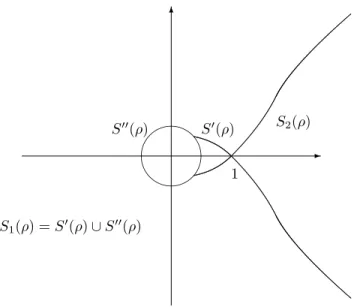
S(ρ) = S1(ρ) ∪ S2(ρ), ρ > 1, where S2(ρ) = {z = reiφ : r ≥ 1, |φ| ≤ π 2ρ, r ρcos(ρφ) − 1 − ρ log r = 0}. (2.26)
6 -&% '$ 1 S00(ρ) S0(ρ) S2(ρ) S1(ρ) = S0(ρ) ∪ S00(ρ)
Figure 2.1: The generalized Szeg¨o’s curve S(ρ).
It will be proved in Chapter 3 that the curve S(ρ) has asymptotes arg z = ±π/(2ρ) (meanwhile the original Szeg¨o’s curve S doesn’t have any asymptote).
Our main result concerning the zero distribution of In(Rnz, λ, E1/ρ) can be
considered as a complete analogue of Szeg¨o’s Theorem J.
Theorem 6 . One has: (i) M0(0, E1/ρ) = S1(ρ),
(ii) M0(1, E1/ρ) = S2(ρ),
(iii) M0(λ, E1/ρ) = S(ρ), for λ 6= 0, 1.
This theorem means that each point on the curve S1(ρ) is an
accumula-tion point of the zeros of sn(Rnz, E1/ρ), each point on the curve S2(ρ) is an
accumulation point of zeros of tn+1(Rnz, E1/ρ), and each point on the curve
S(ρ) = S1(ρ) ∪ S2(ρ) is an accumulation point of the zeros of In(Rnz, λ, E1/ρ),
λ 6= 0, 1. Theorem 6 also answers the question how to continue the curve S(ρ) into
the exterior of the unit disc. Theorem 6 is an immediate corollary of Theorems 7, 8, 9 below.
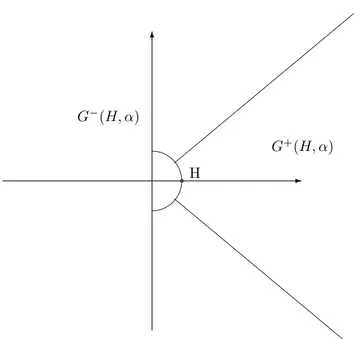
6 -,, ,, ,, ,, ,, ,, l l l l l l l l l l l l &% '$ d 1 Ω5 Ω4 Ω3 Ω1 Ω2 Figure 2.2: Regions Ωi, i = 1, 2, . . . , 5
For given sufficiently small δ1 > 0, δ2 > 0, δ3 > 0 and h > 0, let us introduce
the following regions.
Ω1 = {z = reiφ: δ3 ≤ r ≤ 1, |z − 1| ≥ δ1, |φ| ≤ 2ρπ − δ2,
rρcos(ρφ) − 1 − ρ log r ≥ 0},
Ω2 = {z = reiφ: |φ| ≤ 2ρπ − δ2, rρcos(ρφ) − 1 − ρ log r ≤ −h},
Ω3 = {z = reiφ: e−1/ρ+ h ≤ r, |φ| ≥ 2ρπ + δ2},
Ω4 = {z = reiφ: δ3 ≤ r ≤ e−1/ρ− h, |φ| ≥ 2ρπ + δ2},
Ω5 = {z = reiφ: r ≥ 1, |φ| ≤ 2ρπ − δ2, rρcos(ρφ) − 1 − ρ log r ≥ h}.
(2.27)
The next theorem deals with the zero–free regions of In(Rnz; λ, E1/ρ).
Theorem 7 . Let δ1, δ2, δ3 and h be given sufficiently small positive constants.
Then, for all sufficiently large n, In(Rnz; λ, E1/ρ) has no zeros in ∪5i=1Ωi.
Theorem 7 can be viewed as an extension of the following Theorem 5 from [12] that corresponds to the case λ = 0 (i.e. related to the zeros of sn(Rnz, E1/ρ) =
Theorem O ([12]). Let δ1, δ2, δ3 and h be given sufficiently small positive
con-stants. Then, for all sufficiently large n, sections sn(Rnz, E1/ρ) = In(Rnz, 0, E1/ρ)
has no zeros outside the unit disc and in ∪4
i=1{Ωi∩ {z : |z| ≤ 1}}.
Theorem 7 implies that the zeros of In(Rnz; λ, E1/ρ) may lie only in the
vicinity of the curve S(ρ) and two rays arg z = ±π/(2ρ). Let us consider the functions In(Rnz, λ, E1/ρ) in the neighborhood of points on the curve S(ρ). The
next theorem gives information about the behavior (and, in particular, the zero distribution) of In(Rnz, λ, E1/ρ) in the neighborhood of the point z = 1 on S(ρ).
Theorem 8 . As n → ∞, we have 1 + Ã 2 ρn !1/2 ζ −n n E1/ρ(Rn) o−1 In Rn 1 + Ã 2 ρn !1/2 ζ ; λ, E1 ρ → eζ2 ( erfc(ζ) 2 − λ )
uniformly on every compact set of the ζ–plane.
By Hurwitz’s Theorem, it follows that, as n → ∞, the zeros of In(Rnz, λ, E1/ρ)
approach the zeros of 1
2erfc(ζ) − λ. This theorem was first proved for ρ = 1, λ = 0
in [22] by D.J. Newman and T.J. Rivlin (see Theorem L before). It was proved in the case ρ > 1 and λ = 0 by A. Edrei, E.B. Saff and R.S. Varga (see [12], Theorem 1). Theorem 8 can be viewed as a generalization of all these results. More strict results were obtained in the case ρ = 1 and λ = 1 by C.Y. Yıldırım in [38].
Our next theorem is concerned with the behavior of In(Rnz, λ, E1/ρ) near the
points ξ = ξ(φ) ∈ S(ρ) distinct from the point z = 1.
Theorem 9 . I. Let ξ = ξ(φ), 0 < φ < π
2ρ, be a fixed point on the generalized
Szeg¨o curve S(ρ). Let τ = |ζ|λsin(φρ) − ρφ, and let the sequences {τn}∞ n=1 and
{εn(ζ)}∞n=1 be defined by the conditions τn ≡ τ ρn(mod 2π), −π < τn≤ π, and εn(ζ) = log n 2(1 − ξρ)n − ζ − iτn (1 − ξρ)n. Then, as n → ∞, In ³ Rnξ (1 + εn(ζ)) ; λ, E1/ρ ´ Γ³1 + n ρ ´ Rn nξn(1 + εn(ζ))n → α(ξ)eζ− ξ 1 − ξ, if |ξ| < 1, −β(ξ)eζ− ξ 1 − ξ, if |ξ| > 1, (2.28)
uniformly on every compact set of the ζ – plane, where α(ξ) = (1 − λ)(2πρ)12e ρ+1 2ρ (ξρ−1) and β(ξ) = λ(2πρ)12e ρ+1 2ρ (ξρ−1).
II. Let ξ = e−1ρeiφ, π
2ρ < φ ≤ π, be a fixed point on the circular portion of S(ρ),
and let the sequences {τ0
n}∞n=1 and {ε0n(ζ)}∞n=1 be defined by the conditions τn0 ≡ (n + 1)φ( mod 2π), −π < τn0 ≤ π, and ε0n(ζ) = Ã 1 2− 1 ρ ! log n n − ζ − iτ0 n n + 1 . Then In ³ Rnξ (1 + ε0n(ζ)) ; λ, E1/ρ ´ Γ³1 + n ρ ´ Rn nξn(1 + ε0n)n → γ(ξ)e−ζ − ξ 1 − ξ (2.29)
uniformly on every compact set of the ζ – plane, where γ(ξ) = (λ − 1)(2πe 1−ρ ρ )12 ρ12− 1 ρΓ ³ 1 − 1 ρ ´ .
As was mentioned before, by Theorem 7, the zeros of In(Rnz; λ, E1/ρ) may lie
only in the vicinity of the curve S(ρ) and two rays arg z = ±π/(2ρ). Theorem 9 implies that each point ξ on the curve S(ρ) is an accumulation point of the zeros of In(Rnz; λ, E1/ρ). Indeed, by Hurwitz’s Theorem, the zeros of In(Rnξ(1 + εn(ζ)); λ, E1/ρ) approach the zeros of the limit functions in (2.28), if ξ ∈ S0(ρ) ∪
S2(ρ), and the zeros of In(Rnξ(1 + ε0n(ζ)); λ, E1/ρ) approach the zeros of the limit
functions in (2.29), if ξ ∈ S00(ρ).
The proof of Theorems 7 and 9 is based on the following theorem that deals with the asymptotic expressions for In(Rnz; λ, E1/ρ) in different domains of C.
Theorem 10 . Let δ1, δ2, δ3 be given sufficiently small positive constants, and
ρ > 1. Then, as n → ∞, In(Rnz; λ, E1/ρ)Γ ³ 1 + n ρ ´ Rn nzn = −λρe RρnzρΓ ³ 1 + n ρ ´ Rn nzn (1 + o(1)) − z 1 − z(1 + o(1)), (2.30) if z ∈ {z = reiφ: r ≥ 1, |φ| ≤ π 2ρ, |z − 1| ≥ δ1}, In(Rnz; λ, E1/ρ)Γ ³ 1 + n ρ ´ Rn nzn = (1 − λ)ρe RρnzρΓ ³ 1 + n ρ ´ Rn nzn (1 + o(1)) − z 1 − z(1 + o(1)), (2.31) if z ∈ {z = reiφ: δ 3 ≤ r ≤ 1, |φ| ≤ 2ρπ, |z − 1| ≥ δ1}, In(Rnz; λ, E1/ρ)Γ ³ 1 + n ρ ´ Rn nzn = (λ − 1) Γ³1 − 1 ρ ´Γ ³ 1 + n ρ ´ Rn+1 n zn+1 (1 + o(1)) − z 1 − z(1 + o(1)), (2.32) if z ∈ {z = reiφ: r ≥ δ 3, |φ| ≥ 2ρπ + δ2, }.
In all expressions above, o(1) is uniform with respect to z.
We remark that, in the special case λ = 1, |z| < 1, one can find the asymptotic expression for In(Rnz; 1, E1/ρ) in [12, Lemma 9.2].
Preliminaries
In this chapter we recall some definitions and results that we will need in the sequel.
3.1
One-sided multiply positive sequences
Let
{an}∞n=0, a0 > 0, (3.1)
be a sequence of real numbers. In this section we always assume that the se-quence (3.1) is at least 2-times positive.
Lemma 1 ([26]). Let (3.1) be a 2–times positive sequence. Set n = min{k :
ak = 0}. If n is finite, then ak = 0 for any k ≥ n.
Proof. By the definition of 2-times positivity, we have, for any k > n,
¯ ¯ ¯ ¯ ¯ ¯ ¯ an ak an−1 ak−1 ¯ ¯ ¯ ¯ ¯ ¯ ¯ ≥ 0. 29
Since an= 0, an−1> 0, we conclude that ak= 0. 2
Therefore, a 2-times positive sequence (3.1) is either finite (has only finitely many nonzero terms), or is composed entirely of positive terms.
With (3.1), we associate the generating function (1.1). The fact that se-quence (3.1) is 2–times positive implies that the radius of convergence R(f ) of series (1.1) is nonzero as the following lemma shows.
Lemma 2 Let f ∈ P F2. Then R(f ) > 0.
Proof. If the sequence (3.1) of coefficients of (1.1) has all nonzero terms – the
only case to discuss due to Lemma 1 – we have
¯ ¯ ¯ ¯ ¯ ¯ ¯ an an+1 an−1 an ¯ ¯ ¯ ¯ ¯ ¯ ¯ = anan−1 Ã an an−1 − an+1 an ! ≥ 0. Thus, ½a n+1 an ¾∞ n=0
is a non increasing sequence of positive numbers that implies the existence of the limit
1
R(f ) = limn→∞ an+1
an . 2
By Lemma 1, for all the functions (1.1) generating by 2-times positive infinite sequences (3.1), all their coefficients ak are strictly positive, that allows us to
introduce the positive numbers
ρk = ak−1 ak , k = 1, 2, . . . , (3.2) and δk = ρk ρk−1 = a 2 k−1 akak−2 , k = 2, 3, . . . (3.3)
The next formulas follow from (3.2) and (3.3)
ak = a0 Qk j=1ρj , k = 1, 2, . . . and ak = a0 ρk 1δk−12 δ3k−2. . . δk , k = 2, 3, . . . (3.4)
We have already mentioned that ½a n+1 an ¾∞ n=0
is a non increasing sequence. It implies that {ρn}∞
n=1 is a non decreasing sequence and hence
δk≥ 1, k ≥ 2. (3.5)
It turns out that if sequence (3.1) of positive numbers satisfies a stronger condition than (3.5), namely, δn≥ A > 1, then the corresponding generating function (1.1)
is an entire function of order 0. More precisely, the following lemma holds.
Lemma 3 . Let (1.1) be a formal power series with all positive coefficients
ak > 0. Assume that there exists a constant A > 1 such that
δk ≥ A, k ≥ k0, (3.6)
where numbers δk are defined by (3.3). Then the series (1.1) converges in the whole complex plane C, and
lim sup r→∞ log M(r, f ) (log r)2 ≤ 1 2 log A. (3.7)
Proof. The proof of this lemma is contained in [26], but we present it here for
the reader’s convenience. By (3.4) and (3.6), we have log ak = log a0− k log ρ1−
k
X
j=2
(k − j + 1) log δj ≤ log a0 − k log ρ1
− kX0−1 j=2 (k − j + 1) log δj− k X j=k0 (k − j + 1) log A = −k2 2 log A + O(k), k → ∞. Hence, ak ≤ CDkA− k2 2 , k = 0, 1, 2, . . . , (3.8)
where C and D are positive constants not depending on k. Since A > 1, then limk→∞a1/kk = 0. Therefore the series (1.1) converges in the whole plane. Further,
using (3.8), we have M(r, f ) = ∞ X k=0 akrk ≤ C ∞ X k=0 A−k22 (Dr)k
= C exp à (log Dr)2 2 log A ! ∞ X k=0 exp − log A 2 à k − log(Dr) log A !2 ≤ C exp à (log Dr)2 2 log A ! sup −∞<x<∞ ∞ X k=−∞ exp ( −log A 2 (k − x) 2 ) .
Since the sum of the series under the supremum sign is a periodic function of x (with period 1), its supremum is finite. Hence
M(r, f ) = O Ã exp ( (log Dr)2 2 log A )! , r → ∞, and log M(r, f ) ≤ (log r) 2 2 log A + O(log r), r → ∞. 2
Therefore, there is a close relation between estimates from below on δn and
growth estimates of the corresponding entire functions of order 0.
The definition of multiple positivity is quite complicated. Therefore it is not easy to check whether or not a given sequence is m-times positive using the definition. Here we present the following test of m-times positivity of a finite positive sequences. It turns out that this test is rather effective.
Lemma 4 (Schoenberg’s Theorem ([33])). Let {bk}nk=0 be a finite sequence of numbers. Consider the m matrices
Bk = b0 b1 b2 . . . bn 0 0 . . . 0 0 b0 b1 . . . bn−1 bn 0 . . . 0 0 0 b0 . . . bn−2 bn−1 bn . . . 0 . . . . . . . . . . . . . 0 0 0 . . . . . . . . . bn , k = 1, 2, . . . .m,
where Bk consists of k rows and n + k columns. Assume that the following con-dition is satisfied for k = 1, 2, . . . , m: all k × k–minors of Bk consisting of con-secutive columns are strictly positive. Then the sequence {b0, b1, . . . , bn, 0, 0, . . .}
3.1.1 One-sided sequences having sections with multiply positive terms
In this thesis we do not work with the classes P Fm, m ≥ 3, themselves, but we
study their subclasses Pm ∈ P Fm, m ≥ 3. Recall that series (1.1) belongs to
the class Pm, m ≥ 2, if the truncated sequences {ak}nk=0 are m-times positive for
all sufficiently large n. It is easy to see that the class P F2 coincides with the
class P2. Therefore, for all infinite sequences (3.1) from Pm ⊂ P2 = P F2, m ≥ 3,
the numbers δn, n ≥ 2, are well defined. The next two lemmas from [26] give
us information about sequences {δn}∞n=2 corresponding to the sequences {an}∞n=0
from P3.
Lemma 5 ([26]). Let {ak}n
k=0 = {a0, a1, . . . , an, 0, 0, . . .}, a0 > 0, an > 0,
n ≥ 2, be a 3–times positive sequence. Then (i) for n = 2, we have δ2 ≥ 2;
(ii) for n = 3, we have δn> 1 and
(δn− 1)2 ≥ 1 − 1 δn−1
. (3.9)
Let sequence (3.1) with nonzero terms belong to the class P3. Then there exists
some n0 ≥ 2 such that, for each n ≥ n0, the truncated sequence {ak}nk=0 is 3–
times positive. By Lemma 5, we have δn > 1 for all n ≥ n0, and therefore the
numbers
yn=
1
δn− 1, n ≥ n0, (3.10)
are well defined. Using (3.9), we obtain
y2
n+1 ≤ yn+ 1, n ≥ n0.
Consider the sequence {zn}∞
n=n0 of positive numbers satisfying the recurrence
equation
and the initial condition zn0 = yn0. It is easy to see that
yn≤ zn, n ≥ n0. (3.11)
Lemma 6 ([26]). Let a formal power series (1.1), which is not a polynomial,
belong to P3 and let for all n ≥ n0 the sequences {ak}nk=0 be 3–times positive. Let {zn}∞n=n0 be the sequence of positive numbers satisfying the recurrence relation
z2
n+1 = zn+ 1, n ≥ n0, (3.12)
and the initial condition
zn0 =
1
δn0 − 1
. Then there exists the limit
lim n→∞zn= 1 +√5 2 := c, and we have 1 δn− 1 ≤ zn, n ≥ n0. Moreover,
(i) if zn0 < c, then the sequence {zn}
∞
n=n0 increases;
(ii) if zn0 > c, then the sequence {zn}∞n=n0 decreases;
(iii) if zn0 = c, then zn = c for any n ≥ n0.
Using (3.10), (3.11) and Lemma 6, we obtain that if sequence (3.1) belongs to
P3, then for any given 0 < ε < 1,
δn≥ c − ε, n ≥ n(ε). (3.13)
The estimate (2.4) for functions belonging to Pm, m ≥ 3, follows from (3.13) and
Lemma 3.
In general, it is difficult to check whether sequence (3.1) belong to P Fm, m ≥ 3,
or not. The next lemma from [27] gives a sufficient condition for (3.1) to belong to Q3 ⊂ P F3.
Lemma 7 ( [27]). For a sequence (3.1) to belong to Q3 it is sufficient to satisfy
δn ≥ 2, n ≥ 2.
3.1.2 One-sided sequences having tails with multiply positive terms
Recall that series (1.1) belongs to the class Rm, m ≥ 2, if the sequences {an, an+1, . . .} are m-times positive for all n large enough. By Lemma 2 such
a series always have a positive radius of convergence by 2-times positivity of
{an, an+1, . . .}.
Assuming f ∈ Rm, m ≥ 2, we choose n such that {an, an+1, . . .} is m-times
positive and moreover an > 0. By Lemma 1, ak > 0 for all k ≥ n. This permits
us to introduce the positive numbers
ρk = ak+1 ak , k = n + 1, n + 2, . . . (3.14) Evidently, ak = Qk an j=n+1ρj , k = n + 1, n + 2, . . . (3.15) Let us introduce the numbers
δk = ρk ρk−1 = a2 k−1 akak−2, k = n + 2, n + 3, . . . (3.16)
Since the sequence {an, an+1, . . .} is 2-times positive, we have
¯ ¯ ¯ ¯ ¯ ¯ ¯ ak−1 ak ak−2 ak−1 ¯ ¯ ¯ ¯ ¯ ¯ ¯ ≥ 0, k ≥ n + 2, i.e. a2 k−1 ≥ akak−2, k ≥ n + 2. Therefore, δk ≥ 1, k = n + 2, n + 3, . . . (3.17) It is easy to see that
ak = an ρk−n n+1 Qk j=n+2δjk−j+1 . (3.18)
The next two lemmas from [28] give information about series (1.1) from Rm, m ≥ 3.
Lemma 8 ([28]). Let {an, an+1, . . .} be a 3-times positive sequence with positive coefficients. Then
(δn+2− 1)2 ≥ 1 −
1
δn+3
. (3.19)
Lemma 9 ([28]). Let sequence (3.1) belong to R3. Then there exists an integer
p such that either
(I) for any n ≥ p + 2, δn≥ c, or (II) there exists q ≥ p + 2, δq< c.
In case (I) the assertion (i) of theorem G is valid while in the case (II) the assertion (ii) is.
We will need the following test of m-times positivity that is contained in [28] and which is due to I.J. Schoenberg (see [33]).
Lemma 10 (Schoenberg’s Theorem ([33])). Let {bk}∞k=0 be a sequence of positive numbers. Consider the m matrices
Bν = b0 b1 b2 . . . bν−1 . . . 0 b0 b1 . . . bν−2 . . . 0 0 b0 . . . bν−3 . . . . . . . . . . . . . 0 0 0 . . . b0 . . . ν = 1, 2, . . . , m,
consisting of ν rows and infinitely many columns. Assume that for ν =
1, 2, . . . , m, the matrix Bν satisfies the condition: all its ν × ν–block-minors ( i.e. minors consisting of ν consecutive rows and ν consecutive columns ) are positive. Then the sequence {bk}∞k=0 is m–times positive.
Lemmas 4 and 10 are very similar. However, Lemma 4 deals with finite se-quences {bk}n
k=0 while Lemma 10 deals with infinite sequences {bk}∞k=0.
3.2
Two-sided multiply positive sequences
Let
{an}∞n=−∞, a0 6= 0, (3.20)
be a two-sided infinite sequence of real numbers. In this section we always assume that (3.20) is at least 2-times positive.
Assume that the sequence (3.20) doesn’t coincide with the trivial sequence
{ρn}∞
n=−∞ for some ρ > 0. It turns out (see [20], p.418) that such a 2-times
posi-tive sequence (3.20) generates Laurent series (2.9) that converges in a nonempty annulus 0 ≤ 1/R1 < |z| < R2.
Lemma 11 . Let the sequence (3.20) be 2-times positive. Set
k1 = min{k > 0 : ak = 0}, k2 = max{k < 0 : ak= 0}. Then ak= 0 for all k < k2+ 1 and k > k1− 1.
Proof. Let us show that ak = 0 for all k ≤ k2. Assume k2 > −∞. We have ¯ ¯ ¯ ¯ ¯ ¯ ¯ ak+1 ak2+1 ak ak2 ¯ ¯ ¯ ¯ ¯ ¯ ¯ = −akak2+1≥ 0
for all k < k2. Hence, ak = 0 for all k ≤ k2. That ak = 0 for all k ≥ k1 can be
proved similarly. 2
Without loss of generality we can assume that a2 6= 0 and a−2 6= 0, i.e. k1 > 2
Lemma 11 allows us to introduce the positive numbers δk = a2 k−1 akak−2 , 0 < k < k1, a2 k+1 akak+2, k2 < k < 0. (3.21) Note that δ1 = δ−1.
Lemma 12 . Let sequence (3.20) be 2-times positive and the numbers k1 and
k2 be defined as in Lemma 11. Then δk ≥ 1 for all k, k2 < k < k1.
Proof. For any k , k2 < k < k1, we have ¯ ¯ ¯ ¯ ¯ ¯ ¯ ak−1 ak ak−2 ak−1 ¯ ¯ ¯ ¯ ¯ ¯ ¯ = akak−2(δk− 1) ≥ 0, if 1 ≤ k < k1, and ¯ ¯ ¯ ¯ ¯ ¯ ¯ ak+1 ak+2 ak ak+1 ¯ ¯ ¯ ¯ ¯ ¯ ¯ = akak+2(δk− 1) ≥ 0, if k2 < k ≤ −1. 2
3.3
Power series with sections from P F
∞Now we present the proof of P´olya’ s Theorem E for the reader’s convenience (see also [26]). The condition f ∈ P∞ means (see Chapter 2) that sections (1.2) have
purely negative zeros for sufficiently large n, that is, for n ≥ n1 say. It is well
known that the derivatives of a polynomial having purely real zeros have purely real zeros. Hence, the quadratic polynomial
à d dz !n−2 sn(z, f ) = (n − 2)!an−2+ (n − 1)!an−1z +1 2n!anz 2
does not have any complex zero. This means that the following inequality is valid: (n − 1)a2n−1 ≥ 2nan−2an, n ≥ n1.
6 -,, ,, ,, ,, ,, ,, l l l l l l l l l l l l A C a a l1 l2 Bρ 1
Figure 3.1: Asymptotes l1 and l2.
By the definition of δn, we can rewrite the last inequality in the form δn≥
2n
n − 1 > 2, n ≥ n1.
Now Theorem E follows at once from Lemma 3. 2
3.4
Some asymptotic relations for Mittag-Leffler
func-tions
In Chapter 2 we have pointed out that the zeros of In(Rnz, λ, E1/ρ), ρ ≥ 1, are
closely connected with the curve S(ρ) = S1(ρ)∪S2(ρ). It turns out that the curve
S2(ρ) has asymptotes.
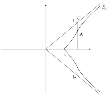
Lemma 13 . The curve S2(ρ) has asymptotes lj =
( arg z = (−1)j−1 π 2ρ ) , j = 1, 2.
Proof. It suffices to consider only the upper half B(ρ) of the curve S2(ρ) (see
Figure 3.1). It is given by the equation
cos ρφ = r−ρ(1 + ρ log r),
which implies that the conditions r → ∞ and φ → π
2ρ are equivalent. Take a point A = (r cos φ, r sin φ) on B(ρ) and a point C =
Ã
r cos φ, r tan π
2ρcos φ
!
on
l1. The distance d(A, l1) from the point A to l1 does not exceed the distance
between the points A and C, i.e.
d(A, l1) ≤ r tan π 2ρcos φ − r sin φ ≤ r sin ρ Ã π 2ρ− φ ! cos π 2ρ = 1 + ρ log r rρ−1cos π 2ρ → 0 as r → ∞. 2 Rewrite (2.19) as In(Rnz; λ, E1/ρ) = (1 − λ)E1/ρ(Rnz) − tn+1(Rnz, E1 ρ). (3.22)
This formula shows that the study of the asymptotic behavior of In(Rnz; λ, E1/ρ)
can be reduced to asymptotic formulas for E1/ρ(Rnz) and tn+1(Rnz, E1
ρ). They
will play a major role in the proof of Theorem 10. Let us present those formulas. The function E1/ρ(z) have the following well–known asymptotic relations (see
[17], p.114): E1/ρ(z) = ρezρ − 1 zΓ³1 − 1 ρ ´ + O Ã 1 |z|2 ! , | arg z| ≤ π 2ρ, |z| → ∞, − 1 zΓ³1 −1 ρ ´ + O Ã 1 |z|2 ! , π 2ρ ≤ | arg z| ≤ π, |z| → ∞. (3.23)