Mean-field renormalization group theory of the t-J model

(1)

MEAN-FIELD RENORMALIZATION GROUP

THEORY OF THE t-J MODEL

a thesis

submitted to the department of physics

and the institute of engineering and science

of bilkent university

in partial fulfillment of the requirements

for the degree of

master of science

By

Cengiz S¸en

(2)

I certify that I have read this thesis and that in my opinion it is fully adequate, in scope and in quality, as a thesis for the degree of Master of Science.

Prof. Dr. M. Cemal Yalabık (Supervisor)

Prof. Dr. Bilal Tanatar

Prof.Dr. Metin G¨urses

Approved for the Institute of Engineering and Science:

Prof. Dr. Mehmet B. Baray

Director of the Institute Engineering and Science

(3)

ABSTRACT

MEAN-FIELD RENORMALIZATION GROUP THEORY

OF THE t-J MODEL

Cengiz S¸en M.S. in Physics

Supervisor: Prof. Dr. M. Cemal Yalabık July, 2002

The quantum nature of the high temperature superconductivity models makes analytical approaches to these systems almost impossible to implement. In this thesis, a computational study of the one and two dimensional t − J models that combines mean-field treatments with renormalization group techniques will be presented. This allows one to deal with the noncommutations of the operators at two consecutive sites of the lattices on which these models are defined. The resulting phase diagram for the 1D t − J model reveals an antiferromagnetic ground state, which may, upon doping with increasing temperature, show striped formation that is seen in the high-Tc cuprates. The qualitative features of the

phase diagram of the 2D case is also presented, which reveals a phase transition between the disordered and antiferomagnetically ordered phases.

Keywords: high-temperature superconductivity, t − J model, Hubbard model,

renormalization group theory, mean-field theory, hard-spin mean-field theory. iii

(4)

¨

OZET

t − J MODEL˙IN˙IN ORTALAMA ALAN

RENORMAL˙IZASYON GRUP TEOR˙IS˙I

Cengiz S¸en Fizik, Y¨uksek Lisans

Tez Y¨oneticisi: Prof. Dr. M. Cemal Yalabık Temmuz, 2002

Yüksek sıcaklık süperiletkenli˘gi modellerinin kuvantum do˘gası, bu sistemlere kar¸sı analitik yakla¸sımları neredeyse olanaksız kılmaktadır. Bu tezde, bir ve iki boyutlu t − J modellerinin, ortalama alan yakla¸sımlarıyla renormalizasyon grup tekniklerini birle¸stiren sayısal bir ¸calı¸sması sunulacaktır. Bu, modellerin tanımlandı˘gı örgünün iki ardı¸sık bölgesindeki operatörlerin yer de˘gi¸stirileme-mesini ele almayı mümkün kılmaktadır. Bir boyutlu t − J modelinin ortaya ¸cıkan faz diyagramı, artan sıcaklıkla katkılama ile antiferromagnetik bazal du-rumun yüksek-Tc materyallerinde görülen ¸cizgili bir dönü¸süm gösterebilece˘gini

ortaya koymaktadır. ˙Iki boyutlu durumun faz diyagramının antiferromagnetik düzenli ve düzensiz fazlar arasındaki faz ge¸ci¸sini ortaya koyan kalitatif özellikleri de sunulmaktadır.

Anahtar kelimeler : y¨uksek sıcaklık s¨uperiletkenli˘gi, t − J modeli, Hubbard

mod-eli, renormalizasyon grup teorisi, ortalama-alan teorisi, sert-spin ortalama-alan teorisi.

(5)

Acknowledgement

I would like to express my gratitude to my supervisor Prof. Dr. M. Cemal Yalabık for his instructive comments and guidance in the preparation of this thesis. I am indebted to him so much, not only in academic issues but also because of his friendly attitude over the last two years.

My thanks also go to Prof. Dr. Bilal Tanatar and Prof. Dr. Metin Gürses for a critical reading of the manuscript and suggesting the necessary corrections. I also would like to thank to M.S. Özge Günaydın for her encouraging support. It is my pleasure to dedicate this and all forthcoming works to my family.

(6)

List of Figures

1.1 A typical phase diagram for high-temperature superconductors. T is the temperature, δ is the doping. . . . 3

2.1 2D CuO2 lattice . . . 8

2.2 Hybridization scheme between Cu − 3dx2_−y2 and O − p_x, p_y orbitals 9

2.3 Formation of bonding between a Cu2+ _{and two O}2− _{ions. Only}

the d electrons of Cu and the px and py orbitals of the oxygens

are considered. The numbers in the parentheses are occupations of the levels in the undoped system[23]. . . 11 2.4 Reduction of the three-band model to the one-band t − J Model. 14 2.5 The spin configuration that is used in the hard-spin mean-field

theory of the 2D Ising model. . . 19 2.6 Magnetization (m) vs. temperature (1/J) for the 2D Ising model.

Jc= 0.3226 to be compared with the exact value Jc= 0.4407. . . 20

2.7 Free energy vs. temperature for the 2D Ising model calculated from the hard-spin mean-field approximation. . . 21

3.1 Hard spins, σ’s, interacting with the three site chain. . . . 26 3.2 Block spin rule: σ’s are the original spins, µ’s are the block spins. 28

(10)

LIST OF FIGURES x

3.3 States that are used in the renormalization group procedure of the 1D t − J model: (a) ferromagnetic state, (b) antiferromagnetic state, (c) empty state, (d) plus-hole state, (e) striped state. . . 29 3.4 A cross section of the phase diagram of the 1D t − J model for

different values of µ/V and J/V . . . . 33

4.1 Block spin configuration that is used in the renormalization group theory of the 2D t − J model. . . . 36 4.2 Examples to the majority rule for the 2D t − J model. . . . 38 4.3 States that are used in the renormalization group procedure of the

2D t − J model: (a) ferromagnetic state, (b) antiferromagnetic state, (c) empty state, (d) plus-hole state, (e) striped state. . . 39 4.4 Forward renormalization of the 2D lattice. . . 40 4.5 Qualitative picture of the phase diagram for the 2D t − J model

(11)

List of Tables

2.1 The estimates for the values in the three-band t − J model in eV’s. 12

3.1 Fixed points that are found from the hard-spin mean-field renor-malization group theory of the 1D t − J model. . . . 32 3.2 Eigenvalues of the linearization matrices corresponding to the fixed

points for the 1D t − J model. . . . 32

4.1 Fixed points that are found from the mean-field renormalization group theory of the 2D t − J model. . . . 42 4.2 Eigenvalues of the linearization matrices corresponding to the fixed

points for the 2D t − J model. . . . 42

(12)

Chapter 1 INTRODUCTION

The announcement of the first high-Tc cuprate in 1986 by J. G. Bednorz and

K. A. Muller[1] at a temperature of 30 K opened a new era in superconductiv-ity. Although superconductivity is known since 1913 from a series of experiments performed by Heike Kamerlingh Onnes[2], the new superconductors were quite different than the old ones, mainly because these superconductors were oxides rather than metals. At first the results seemed unexpected, but the confirmation later came with even higher transition temperatures by Takagi et. al.[3] in 1987. This work made it possible to use inexpensive and easily available nitrogen instead of expensive and complex helium cooling systems in order to achieve superconduc-tivity. Afterwards, the transition temperature has risen dramatically, examples are Y Ba2Cu3O7 with Tc=94 K (the first superconductor having Tc greater than

the boiling temperature of nitrogen, T =77,4K) (1987), a mercury based copper oxide material with Tc=133 K (1993), again a mercury based copper oxide with

Tc=166 K (1996).

Theoretical studies concerning high temperature superconductivity have gained acceleration over the past years with the development of new ideas as well as the exponential growth of the computing technology. However, the mech-anism of superconductivity in these materials remains mysterious in the sense that the conventional BCS theory of superconductivity[4] cannot be applied to these materials. The reason for that lies behind the fact that in the BCS theory,

(13)

CHAPTER 1. INTRODUCTION 2

the coherence length associated with the average size of a Cooper pair is large (∼500˚A–10000˚A) with respect to that of high-Tc compounds (∼12˚A–15˚A). Thus,

for high-Tc cuprates, the application of standard mean field techniques may not

reveal the real physics of the problem. However, the central idea of the BCS theory, which is the pairing of electrons, is still used to find out some properties of high-Tc materials.

In the search for a Hamiltonian to describe the behavior of these materials, the one-[5] and three-band Hubbard models[6, 7, 8] and the t-J model[9] were pro-posed. Although these models are results of great simplifications, they are now in the center of theoretical studies. The theories that combine the pairing ideas with strong antiferromagnetic correlations seen in the cuprates contain spin-bag type theories[10, 11, 12], antiferromagnetic Fermi-liquid theories[13], and dx2_−y2

theories [14, 15]. In the spin-bag type theories, superconductivity is explained based on the observation that in these materials there exists an antiferromagnetic spin ordering over distances large compared to lattice spacing. This spin correla-tion produces an electronic pseudogap ∆SDW which is locally suppressed by the

addition of a hole. This suppression in turn forms a bag inside which the hole is self-consistently trapped. Then these holes are attracted by sharing a com-mon bag, and this pairing interaction Vk−k0 leads to a superconducting energy

gap ∆SC which is nodeless over the Fermi surface. In ref.[13], the

antiferromag-netic correlation length of 2,5 lattice constants is found for a phenomenological model of a one-component system of antiferromagnetically correlated spins. It is shown that all of the available normal state NMR and NQR measurements in the

Y Ba2Cu3O7 are quantitatively well-explained by this model. The calculations

based on the pairing mechanism that involve antiferromagnetic spin fluctuations support the proposal that high-Tc superconductors possess a dx2_−y2-type

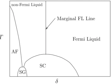
symme-try in the superconducting state, as opposed to s-wave symmesymme-try seen in normal superconductors. It has been shown that[15], this highly-anisotropic state is con-sistent with NMR measurements. A typical phase diagram for high-Tc materials

is shown in Figure 1.1. The antiferromagnetic phase dominates near half-filling, and is superseded by superconductivity (SC) at higher dopings, often by way of spin glass (SG) phase. At extreme overdoping, the material becomes a metal.

(14)

The underdoped normal state exhibits many anomalous properties which are in-dicative of its non-Fermi Liquid nature.

SC AF SG Marginal FL Line Fermi Liquid non-Fermi Liquid

T

δ

Figure 1.1: A typical phase diagram for high-temperature superconductors. T is the temperature, δ is the doping.

Theories that do not use the pairing ideas treat the excitations as spinons and holons[16]. Spinons have zero charge and spin 1/2, whereas holons have the charge e and spin 0. In this direction the 1D Hubbard model has been dis-cussed by Anderson[17]. Among the other approaches to the high-Tc

superconduc-tivity are anyon superconducsuperconduc-tivity[18, 19, 20], gauge theories[21], and marginal Fermi-Liquid theories[22]. In anyon superconductivity theories, it has been men-tioned that a spinon carrying half-fermion statistics plausibly binds to any in-troduced hole and creates a spinless charged half-fermion composite. Then, two half-fermions can pair to make a boson, which is a good candidate for a supercon-ducting condensate. It has also been shown that[20], these pairs are energetically favorable. A fluctuating gauge field scatters holes strongly and the superconduc-tivity coincides with the onset of coherence among the holes[21]. It is claimed that[22] the normal state anomalies in the Cu-O high-Tc superconductors follow

from the fact that there exists spinon and holon excitations with the absorptive part of the polarizability at low frequencies ω proportional to ω/T and constant otherwise. This hypothesis characterizes these materials in the normal state as marginal Fermi-liquids and leads to an attractive particle-particle interaction for superconductive pairing. Other approximations such as perturbative calculations

(15)

in bubble and ladder diagrams, as well as self-consistent ones (mainly mean-field-like) have results that are difficult to judge their results as to their closeness to the actual properties of the models[23].

Although all of the aforementioned approaches helped in many ways in under-standing different aspects of these materials, the difficulty in the solutions of the

t − J and the Hubbard models prevents a clear-cut theory for high-temperature

superconductivity. As yet, only one-dimensional cases of these models are fully understood[25, 26], which are not so interesting because of the 2D nature of the problem. However, even in 1D, Ogata et. al. showed that[26] there exist a region in the parameter space where superconducting correlations become dom-inant. The solution of Ref.[26] utilizes exact diagonalization and exact solutions at J/t = 0 and 2. It is shown that phase separation takes place above a critical value of J around Jc = 2.5 − 3.5 depending on the electron density. There is

no phase separation in the 1D Hubbard model. The phase- separation in the 2D

t − J model is investigated using high-temperature series expansion by Putikka et. al. through tenth order[27]. It was shown that the phase separation is quite

different than the 1D case, since in one-dimension the phase-separation line is in the relatively narrow range between J/t = 2.7 as n → 0 and J/t = 3.5 at half-filling, whereas in 2D it extends from J/t = 3.8 as n → 0 to J/t = 1.2 near half-filling. Also the slope of the phase-separation line in the 1D case is positive, whereas it is negative in the 2D case[27, 28]. For a complete list of references regarding the early times of high-temperature superconductivity theories, refer to the review article by Dagotto[23].

More recent approaches to the t − J model focus on the configuration of electrons and holes in the superconducting state. One possible candidate is the so-called striped phase, where electrons and holes arrange themselves in such a way that the configuration goes as two electrons one with spin up and the other with spin down followed by two holes. This state has been examined by many groups with numerous techniques, both analytically as well as numerically. Among them are density matrix renormalization group (DMRG) studies[29, 30], exact diagonalization techniques[31], and computational studies[32, 33]. In the density matrix renormalization group study of the 2D t − J model, a striped

(16)

phase is found at a hole doping of x = 1/8 on clusters as large as 19 × 8[29]. At the same hole doping, it was shown that[31] the low-energy states of the 2D t − J model are uniform, whereas the excited states with charge density wave structures could be interpreted as striped phases. Computational studies indicate that[32] the elementary stripe “building block” resembles the properties of one hole at small J/t, with robust AF correlations across the hole induced by the local tendency of the charge to separate from the spin. Thus, it is argued that the seed of half-doped stripes already exists in the unusual properties of the insulating compounds.

In the next chapter, the models of high-Tc superconductivity and the

hard-spin mean-field theory are discussed, the latter of which constitutes an important aspect of the approximation that is used in this thesis. Due to the quantum nature of the problem, one should be very careful in handling the models that are mentioned above. The hamiltonians of these models consists of operators that does not commute at the two consecutive sites of the lattice on which all these hamiltonians are defined. This clearly makes a conventional renormalization group calculation questionable. Thus, in the third chapter, a way to overcome this difficulty is presented with an application to the 1D t−J model. This method combines the hard-spin mean-field theory with the block-spin transformation of renormalization theory, yielding a finite temperature phase diagram for the 1D

t − J model. In the fourth chapter, a similar approach is applied to the 2D case,

this time with mean-field theory instead of the hard-spin mean-field theory, due to some limitations discussed in the text. In the last chapter, we conclude with the results.

(17)

Chapter 2 THEORETICAL

BACKGROUND

In this chapter, theoretical background that is necessary for the following chapters will be elucidated. The chapter starts with the Heisenberg model and continues with the Hubbard model and the t − J model. The reduction of the Hubbard model to the one-band t − J model in the strong coupling regime will also be presented. Mean-field theory and renormalization group theory are examples of general theories about which the reader can find information easily[39]. For this reason, this chapter contents with the hard-spin mean-field theory and closes with an application to the 2D Ising model.

2.1 Heisenberg Model

Strong antiferromagnetic correlations are dominant in high-Tc cuprates. It is

this feature of these materials that makes necessary to study first the spin-spin interaction term, i.e. the Heisenberg term, before going on with the Hubbard model and the t − J model. Indeed, both of these models include the Heisenberg term. The Heisenberg hamiltonian put spins on a square lattice and lets the spins interact with a vector interaction[24]. In the most general form, the Heisenberg

(18)

CHAPTER 2. THEORETICAL BACKGROUND 7

model is defined as:

H = X hiji JijSi· Sj = X hiji Jij(SixSjx+ SiySjy+ SizSjz). (2.1)

where Jij is the interaction constant between the spin at the ith site and the

spin at the jth site. In general the summation is taken over all sites hiji, but for simplicity, one takes into account only the nearest neighbor interaction and treats the system as an isotropic one. In this case J is a constant and can be taken outside the summation:

H = JX

hiji

Si· Sj (2.2)

In this convention, J is positive for antiferromagnetic interaction and negative for ferromagnetic interaction. Note that Heisenberg model reduces to the Ising model in the absence of Sx and Sy terms, and reduces to the XY model in the

absence of the Sz term. It is possible to write this hamiltonian in many ways,

e.g. in the ladder representation, defining:

Six =

1

2(Si++ Si−), Siy=

−i

2 (Si+− Si−), (2.3) it is possible to write the Heisenberg hamiltonian as:

H = J

2 X

hiji

(Si+Sj−+ Si−Sj++ 2SizSjz) (2.4)

The operator(s) Si+ (Si−) can be thought of as creating (destroying) a spin up

(down) electron at site i. The Heisenberg model is often solved for spin greater than one-half or for coupling between spins which may be further neighbors. Here the word solve means “approximately solve”, since it has not been solved exactly, except in one dimension[25].

(19)

2.2 Hubbard Model

2.2.1 Three-Band Model

i

i+

cy

i+

cx a 2 Cu ≡ O ≡ a

Figure 2.1: 2D CuO2 lattice

Emery first suggested that[6] the electronic structure of the CuO2 planes

can be described by a Hubbard Hamiltonian on a 2D-lattice having one Cu site and two O sites per unit cell shown in Figure 2.1. A single 3dx2_−y2 orbital in

each Cu site as to become hybridized with each of the four 2px, 2py orbitals of

the surrounding O sites pointing toward the i-site, as shown in Figure 2.2. In addition, a strong Coulomb repulsion term is present when two electrons happen to be both in the 3d orbital at the same site i. A hamiltonian describing the above interactions is of the form:

H = X iσ ²dd†iσdiσ+ U X i ni↑ni↓+ X µσ X α ²ppα†µσpαµσ + X iσ X µi (Viµd†iσpµiσ+ h.c.). (2.5)

where the Latin indices label sites on an arbitrary lattice, σ =↑, ↓ is a spin index (for spin-1/2 fermions) and i and µ denote, respectively, the Cu sites and the

O sites; d†_iσ, pα†

µiσ create electrons with spin σ in the Cu(3dx2−y2) and O(2px) or

(20)

µi = i ± cy runs over the four O−sites around the Cu−site i and, according to

the hybridization scheme of Figure 2.2, it is understood that the pµiσ’s indicate

px

µiσ and p

y

µiσ for µi = i ± cx and µi = i ± cy respectively.

-+

+

-

+

-+

-V

+V

+

-py px dx2_−y2

Figure 2.2: Hybridization scheme between Cu − 3dx2_−y2 and O − p_x, p_y orbitals

The hybridization matrix element Viµ is assumed to be proportional to the

overlap of the corresponding 3d and 2p orbitals and has then the form

Viµ= (−1)αiµV (2.6) with αiµ = ( 1 for µi = i + cx; µi = i + cy; 0 for µi = i − cx; µi = i − cy. (2.7)

(21)

2.2.2 One-Band Model

A more simpler, one-band, version of the Hubbard model is defined by the many-body hamiltonian: H = −X ij X σ tijc†iσcjσ+ 1 2 X ijkl X σσ0 hij|v|klic†_iσc†_jσ0clσ0c_kσ (2.8)

where the ciσ and c†iσ are electron annihilation and creation operators, tij is the

hopping integral between the sites i and j, and v is the two-body Coulomb po-tential. For simplicity, one considers only the nearest neighbor (n.n.) hopping:

tij =

(

t (i, j) = n.n.

0 otherwise (2.9) and screened interactions:

hij|v|kli =

(

U i = j = k = l

0 otherwise (2.10) For a single band, this implies σ0 _{= −σ ≡ ¯}_{σ, and the simplest version of the}

model becomes: H = −tX hiji X σ c†_iσciσ+ U X i ni↑ni↓, (2.11)

where niσ = c†iσciσ and hiji denotes a sum over n.n. ordered pairs.

2.3 t − J Model

2.3.1 Three-Band Model

Due to very strong Cu − O bonds on the planes, the basic assumption in writing a hamiltonian to describe the high-Tc materials is to restrict the consideration

in electrons moving on the CuO2 planes. The Cu2+ ions have nine electrons in

(22)

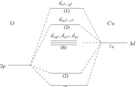
be simplified by taking into account that every Cu atom is surrounded by a O atom as shown in Figure 2.1. The copper and oxygen orbitals can be shown to separate, and the state with highest energy is a d_x2_−y2 wave carrying the missing

electron which gives the ion its spin-1/2. This is schematically illustrated in Figure 2.3. Thus, with one hole per unit cell (i.e. in the absence of doping), the planes can be described by a model of mostly localized spin-1/2 states that gives these materials their antiferromagnetic character. The other energy levels are occupied, and as a first order approximation, they can be neglected. It has

(1) (6) (2) (2) (2) 2p O Cu 3d dxy0, d_xz0, d_yz d3z2_−r2 εd dx2_−y2

Figure 2.3: Formation of bonding between a Cu2+ _{and two O}2− _{ions. Only}

the d electrons of Cu and the px and py orbitals of the oxygens are considered.

The numbers in the parentheses are occupations of the levels in the undoped system[23].

been mentioned before that high-Tccompounds are indeed insulators with strong

antiferromagnetic correlations in the presence of doping. In order for this to be preserved, upon doping, the double occupancy of the d_x2_−y2 orbital must be

energetically unfavored, hence giving the material its antiferromagnetic character. Then, the three band model can be written as[6, 7, 8] (with the vacuum defined

(23)

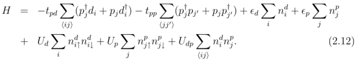
as filled Cud10 _{and Op}6 _states):

H = −tpd X hiji (p†_jdi+ pjd†i) − tpp X hjj0_i (p†_jpj0 + p_jp†_j0) + ²d X i nd_i + ²p X j np_j + Ud X i nd i↑ndi↓+ Up X j np_j↑np_j↓+ Udp X hiji nd inpj. (2.12)

Indeed, this is an extended Hubbard model, where pj’s are fermionic operators

that destroy holes at the oxygen sites labeled j, di’s the similar operators for

the copper sites labeled i. The terms tpd and tpp correspond to the hopping

amplitudes between Cu − O and O − O, respectively. Ud and Up are Columbic

repulsions when two electrons happen to be at same d and p orbitals and Upd is

the Columbic repulsion between a Cu site and a O site. The O − O hopping term

tpp and the repulsion term Up are introduced for completeness and they can be

neglected in reduction to the one-band model. In the strong coupling limit this model reduces to the Heisenberg model with a superexchange antiferromagnetic coupling[8]. Typical values of the parameters in the Hamiltonian is given in Table 2.1.

²p− ²d tpd tpp Ud Up Upd

3.6 1.3 0.65 10.5 4 1.2

Table 2.1: The estimates for the values in the three-band t − J model in eV’s.

2.3.2 One-Band Model

Zhang and Rice introduced a single-band hamiltonian in order to describe the superconducting CuO2 planes[9]. Their main reasoning is based on hybridization

that strongly binds a hole on each square of O atoms to the central Cu2+ _ion

to form a local singlet. Then, this singlet moves through the lattice of Cu2+

ions in a similar way as a hole in the one-band effective hamiltonian. Here, it is important to make the distinction between holes and vacancies. A vacancy is a missing oxygen atom, while a hole is an oxygen atom with charge -1 instead of

(24)

-2[34]. With the removal of the terms introduced for completeness and the term corresponding to the Columbic repulsion between a Cu site and a O site, the hamiltonian in Equation 2.19 becomes:

H = −tpd X hiji (p†_jdi+ pjd†i) + ²d X i nd i + ²p X j np_j + Ud X i nd i↑ndi↓. (2.13)

Consider the case when the atomic energy of the Cu holes ² = 0 and ² > 0. The hybridization matrix, tpd, is assumed to be proportional to the wave-function

overlap of the Cu and O holes. It is also assumed to be constant and taken outside of the summation. Taking into account of the phase factor, and assuming the Cu − Cu distance is the lattice constant, one can write it as:

−tpd = (−1)nt,pt0, (2.14)

where t0 is the amplitude of the hybridization, np,d = 2 if l = i −1₂x or l = i −ˆ 1₂y,ˆ

and np,d = 1 if l = i+1₂x or l = i+ˆ 1₂y. In the absence of doping, the Laˆ 2CuO4 has

1 hole per Cu. At t0 = 0, all the Cu sites are singly occupied, and all the O sites

are empty in the hole representation. When t0 is small, then the virtual hopping

processes involving the doubly occupied Cu hole states produces a superexchange antiferromagnetic interaction between neighboring Cu sites, and the model is well described by the Heisenberg model:

H = JX hiji Si· Sj, J = 4t4 0 ²2 p (1 U + 1 2²p ). (2.15)

Here the summation is taken over nearest-neighboring sites, and S’s are spin-1 2

operators. Consider the copper ion surrounded by four oxygen hole states shown in Figure 2.2. The states of the holes can be either symmetric or antisymmetric with respect to the central Cu ion. When combined with the Cu hole, these states form singlet and triplet states. To the second order in perturbation theory about the atomic limit, the energy of the spin singlet state has the lowest energy[9], and hence it is possible to work in the subspace of the spin singlet state, without changing the physics of the problem. This effectively corresponds to replacing the hole originally located at the oxygen by a spin singlet state centered at the

(25)

Cu-site. In turn, the model is equivalent to electrons and spinless holes moving

on a 2D square lattice shown in Figure 2.4.

=⇒ O ≡

Cu ≡ e−_≡ hole ≡

Figure 2.4: Reduction of the three-band model to the one-band t − J Model.

The one-band t − J model can now be written as:

H = −tX

hiji,σ

[(1 − ni−σ)c†iσcjσ(1 − nj−σ) + (1 − ni−σ)ciσc†jσ(1 − nj−σ)]

+ JX

hiji

[Si· Sj −

1

4ninj]. (2.16) where Si are spin-1/2 operators at the sites i of the 2D lattice, and J is the

antiferromagnetic interaction between the nearest neighbors sites. The hopping t term corresponds to the kinetic energy that allows the movement of the electrons in the lattice. The doubly occupied sites are not allowed and are projected out by the operators (1 − ni−σ). With this definition, one considers only three possible

states per site, i.e. an electron with spin up or down or a hole. It is clear that in the absence of doping, i.e. t = 0, the model reduces to the Heisenberg model of interacting fermions in a 2D lattice.

It has to be mentioned that the reduction of the three-band model to the single-band model is still controversial and in the past it has been a subject of debate[35, 36, 37]. There is also another version of the t − J model, the so-called

(26)

extended t − J model which is defined by:

H = tX hiji,σ (c†_iσcjσ + ciσc†jσ) + t0 X hiki,σ (c†_iσckσ + ciσc†_kσ) + JX hiji [Si · Sj− 1 4ninj]. (2.17) where the t0 _{term is introduced to include the next-nearest neighbor hoppings.}

Again, it is understood that the doubly-occupied sites are not allowed. Although the extension can be generalized, in what follows, we shall assume that t − J model of the Equation 2.23 can be used to describe the cuprates, and the higher order terms are small enough that they can be neglected.

2.4 Strong Coupling Limit of the One Band

Hubbard Model

The Hubbard model is mainly studied in the strong coupling limit in the high-temperature superconductivity community. However, in this limit, this model reduces to the t − J model as will be shown below. Hence, one can restrict himself to the t − J model only.

Consider the one-band Hubbard model written as (this discussion follows that of Ref.[40]):

H = H0+ V, (2.18)

where H0 is the hopping term and V = U

P

ini↑ni↓. Let Hn be the eigenspace of

V with exactly n doubly occupied sites, corresponding therefore to the eigenvalue En= nU. The projectors Pn onto Hn can be generated by expanding:

Π(x) = N Y i=1 [1 − (1 − x)ni↑ni↓] = N X n=0 xn_P n, (2.19)

(27)

where 0 ≤ x ≤ 1 and N is the number of sites in the lattice. In particular, the Gutzwiller projector which is defined as:

P0 =

N

Y

i=1

(1 − ni↑ni↓) (2.20)

selects the subspace containing no doubly-occupied sites at all, i.e. ni ≤ 1 as an

operator inequality. One can as well define operator projecting onto the subspace containing at least one doubly-occupied site:

Pα≡

X

n≥0

Pn. (2.21)

Clearly, P0+ Pα = ˆ1. Using the decomposition of identity, one can write:

H0 ≡ P0H0P0 + PαH0Pα+ P0H0Pα+ PαH0P0, (2.22)

and

V ≡ PαV Pα. (2.23)

It is trivial to check that: P0H0Pα = P0H0P1 and PαH0Pα = P1H0P0. Using

the identity ciσ ≡ ciσ[(1 − ni¯σ) + ni¯σ], one can write H0 as[38]:

H0 ≡ Th+ Td+ Tmix, (2.24) where: Th = −t X hiji,σ (1 − ni¯σ)c†iσcjσ(1 − nj ¯σ); ¯σ = −σ (2.25) Td = −t X hiji,σ ni¯σc†iσcjσnj ¯σ (2.26) Tmix = −t X hiji,σ

(28)

With these definitions of the terms in the one-band Hubbard model, we can write:

H = H˜0+ Hα, where: (2.28)

˜

H0 = P0H0P0+ PαH0Pα+ V (diagonal term), (2.29)

Hα = P0H0Pα+ PαH0P0 (off-diagonal term). (2.30)

In order to find a canonical transformation eliminating the effect of Hα to lowest

order, i.e. such that the transformed hamiltonian satisfies P0Hef fPα = 0 to the

required order, one can start with the formal definition:

H(λ) = ˜H0 + λHα, (2.31)

and seek a canonical transformation of the form:

U(λ) = eiλS_; _{S = S}†_, _(2.32)

where S has to be such that the transformed hamiltonian Hef f(λ) obeys:

Hef f = eiλSH(λ)e−iλS = ˜H0+ O(λ2). (2.33)

Expanding Equation 2.40 in terms of λ, one gets:

Hef f(λ) = ˜H0+ λ(Hα+ i[S, ˜H0]) + λ2(i[S, Hα] +

1

2[S, [ ˜H0, S]]) + O(λ

2_{), (2.34)}

where S is determined from:

[ ˜H0, S] + iHα = 0. (2.35)

Hence, up to terms of order t2 _{(setting λ = 1), one finds:}

Hef f = ˜H0+

i

2[S, Hα]. (2.36) In the low-energy limit with doubly occupied states are projected out by the

(29)

Gutzwiller projector P0, the effective hamiltonian Hef f is given by[38]:

P0Hef fP0 = P0Hˆef fP0 with ˆ Hef f = Th+ H(1)+ H(2), (2.37) where: Th = −t X hiji,σ (1 − ni¯σ)c†iσcjσ(1 − nj ¯σ), (2.38) H(1) = 2t2X hiji X τ σ

(1 − ni¯σ)c†iσcjσnj ¯σnj ¯τc†jτciτ(1 − ni¯τ), (2.39)

H(2) _{= t}2X

hijli

X

τ σ

(1 − ni¯σ)c†iσcjσnj ¯σnj ¯τc†jτclτ(1 − nl¯τ) (2.40)

and hiji denote nearest neighbors, while i and l are nearest neighbors to j. Indeed, the second term suggest the extended t − J model touched upon in the previous section. Neglecting the second term and rearranging the first two terms with the definitions made for the S operators in Section 2.1, one gets the one-band t − J model: Ht−J = −t X hiji,σ (1 − ni¯σ)c†iσcjσ(1 − nj ¯σ) + JX hiji {Si· Sj− 1 4ninj} (2.41) as the strong coupling limit of the one-band Hubbard model. Thus, instead of studying the strong coupling limit of the Hubbard model, one can safely deal with the t − J model.

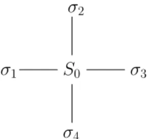
2.5 Hard-Spin Mean-Field Theory

In the conventional mean-field theory of spin systems, a spin feels the effective field produced by the magnetizations of the nearby spins. This is clearly not the case in reality, since a given spin should feel the effective field which is determined

(30)

by the full spins (σi = ∓1) of its neighbors. Hard-spin mean-field theory is

developed[41] in order to fully incorporate this fact and is shown to yield very satisfactory results for various models[41]. To illustrate the basics of the theory, consider the spin−1/2 ferromagnetic Ising model defined with the hamiltonian

H = −JP_hijiSizSjz + h

P

iSiz, where h is the external field. For simplicity,

consider the case when h = 0. In the lattice shown in Figure 2.5, the real spin in

S0

σ2

σ3

σ4

σ1

Figure 2.5: The spin configuration that is used in the hard-spin mean-field theory of the 2D Ising model.

the middle is coupled to hard-spins at the boundary denoted with Greek letters. Instead of the mean-field result for the magnetization m = tanh(JP_imi),

hard-spin mean-field theory uses:

m = tanh(JX

i

σi), (2.42)

where σi = ∓1 with probability:

Pi(σi) =

1 + σimi

2 , (2.43)

where mi = hSizi is the local magnetization. However, in our case the interaction

is isotropic and this gives mi = hS0i ≡ m. The probability in Equation [2.43] is

found by writing the most general form and then minimizing it with respect to the constraints P_iPi = 1 and

P

iPiσi = m. The sum in Equation 2.42 is over

all neighboring spins. The equation for the magnetization then becomes:

m =X {σi} Y i µ 1 + σim 2 ¶ tanh(JX i σi), (2.44)

(31)

where the sum {σi} is over all interacting neighbor spin configurations. The index

i runs from 1 to 4 in the present case. This gives a self-consistent equation for the

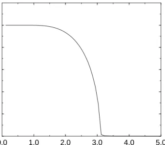
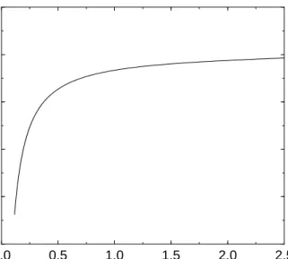
magnetization. A similar equation can be written for the partition function from which one can extract various information like entropy, free energy, etc. These equations are solved numerically for the magnetization and partition function. In Figure 2.6, the results for the magnetization and the free energy are summarized. It is seen that the critical temperature at which the spontaneous magnetization sets is Jc = 3.226. The conventional mean-field result for Jc is 0.25, whereas

the exact result is 0.4407. Thus, even in such a simple case considered above, the hard-spin mean-field theory gives more correct results that the conventional approach where the effective field is determined by magnetizations instead of hard-spins.

The hard-spin mean-field theory is used in the renormalization group theory of the 1D t − J model in the next chapter. However, because of computational difficulties, it is hard to implement it in the 2D case. This issue will be discussed further in the fourth chapter.

0.0 1.0 2.0 3.0 4.0 5.0 Temperature, 1/J 0.0 0.2 0.4 0.6 0.8 1.0 Magnetization, m

Figure 2.6: Magnetization (m) vs. temperature (1/J) for the 2D Ising model.

(32)

CHAPTER 2. THEORETICAL BACKGROUND 21 0.0 0.5 1.0 1.5 2.0 2.5 Temperature, 1/J −40.0 −30.0 −20.0 −10.0 0.0 10.0 F=−ln(Z)

Figure 2.7: Free energy vs. temperature for the 2D Ising model calculated from the hard-spin mean-field approximation.

(33)

Chapter 3 ONE-DIMENSIONAL t-J

MODEL

Although it is believed that high-temperature superconductivity is related to 2D

CuO2 planes, the 1D t−J model also reveals some indications of superconducting

correlations in the physically allowable region of the parameter space. The phase diagram of the 1D t − J model is now widely understood [26], but the problem with the higher dimensions is still open. Ogata et. al.’s results show that phase separation takes place above a critical value of J around Jc/t = 2.5 − 3.5

de-pending on the electron density. They also mention that in the small J region the Tomonaga-Luttinger liquid theory holds and that the superconducting corre-lations become dominant between the exactly solvable case (J/t = 2) and phase separation. As Anderson claimed[16] 2D strongly correlated electronic systems could share some properties of 1D case. In this chapter, the results of a hard-spin mean-field theoretical renormalization group technique for the 1D t − J is presented. We have found ordered and disordered phases separated by a phase separation line that is showed in the 1/V − t/V space. The character of the order is dependent upon the values of V /J and µ/J. The main program used in this study is given in Appendix A.1.

(34)

CHAPTER 3. ONE-DIMENSIONAL t-J MODEL 23

3.1 Motivation

The non-commutativity of the operators at the two consecutive sites of the lattice on which the t − J hamiltonian is defined does not allow one to apply standard renormalization group techniques such as block-spin transformation and Migdal-Kadanoff renormalization group procedure. To illustrate this fact, consider 1D

t − J hamiltonian defined as:

−βH = X i [−βH(i, i + 1)], (3.1) with H(i, j) = −t X hiji,σ (c†_iσcjσ+ c†jσciσ) − J X hiji Si· Sj + V X hiji ninj+ µ X i ni (3.2)

where t is the hopping amplitude, J is the spin-spin interaction constant (+ for antiferromagnetic, − for ferromagnetic interaction), V stands for the Coulomb interaction, ciσ destroys an electron at site i with spin σ, the number operator

niσ = c†iσciσ and Si are the electron density and spin operators at site i, and

ni = ni↑+ ni↓. Note that the conventional t − J hamiltonian is obtained when

V /J = 1/4. Doubly occupied sites are not allowed and they can be thought of as

projected out by a projection operator P defined as:

P = Πi(1 − ni↓ni↑) (3.3)

In what follows, the + sign and ↑ as well as − sign and ↓ will be used inter-changeably. Now, suppose a renormalization group-transformation in which the renormalization is achieved by taking the trace over the even-numbered sites. In exact form this transformation can be written as[42]:

hu1u3u5. . . |e−β 0_H0 |v1v3v5. . . i = X w2w4w6... hu1w2u3w4u5w6. . . |e−βH|v1w2v3w4v5w6. . . i, (3.4)

(35)

where u1, w2, v3 etc. represent the single-site states. Primes indicate the

renor-malized system. Although this renormalization conserves the partition function, it cannot be implemented due to the non-commutativity of the operators in the hamiltonian. An approximation of the form:

Treven statesexp(−βH) = Treven statesexp

Ã_even X i −βH(i − 1, i) − βH(i, i + 1) ! ' even_Y i

Treven sitesexp(−βH(i − 1, i) − βH(i, i + 1))

= even_Y i exp(−β0_H0_{(i − 1, i + 1))} ' exp Ã even X i −β0_H0_{(i − 1, i + 1)} ! = exp(−β0H0), (3.5) has been applied to t−J model[43] and gave no finite temperature phase transition in 1D. This approximation consists in ignoring, in two formally opposite direc-tions, the noncommutations of operators between the two consecutive segments of the unnormalized system. Hence, an application of such an approximation is questionable. Instead, consider a three-site cluster that couples to the boundary with the Hartree-Fock approximated form of the interaction which is defined as:

AB = hAiB + AhBi − hAihBi, (3.6) and then continue with a block spin transformation, the details of which will be explained in the subsequent sections. This allows one to handle the problem taking into account the commutators between the operators at the boundary.1

The approximation discussed here is a general one and can be applied to all lattice hamiltonians defined in arbitrary dimensions. In this chapter, it is applied to the 1D t − J model and in the following chapter it is applied to the 2D t − J model with minor differences from that of the 1D case.

1_{Indeed, this may be thought of as being equivalent to replacing the commutator of two} operators by a c-number, instead of the zero value emerging from the approximation discussed in the text.

(36)

3.2 Hard-Spin Mean-Field Treatment of the

Boundary

In order to evaluate the matrix elements of the t − J hamiltonian, it is convenient to express both Si and ni in terms of creation and annihilation operators c†iσ and

ciσ. To do this one can define two other spin operators such that one of them

first destroys an electron having spin ↓ at site i and then creates an electron with spin ↑ at the same site. Such an operator may be denoted as Si+ and in terms

of the creation and annihilation operators it becomes Si+ = c†i+ci−. Similarly one

can define the operator Si− = c†i−ci+, i.e., destroying an electron having spin ↑

and creating a new one with spin ↓ at site i. Since

Si = Sixˆx + Siyˆy + Sizˆz, (3.7)

in the S2_{− S}

z basis, one can define:

Six = 1 2(Si++ Si−), Siy= −i 2 (Si+− Si−), Siz = 1 2(ni++ ni−). (3.8) It is seen that in this basis, the only contribution to the off-diagonal elements in the hamiltonian comes from the hopping term and the x- and y- components of the spin operator.

The operators defined above are used to generate the matrix elements of the

t − J hamiltonian for a three-site chain coupled to the boundaries with

hard-spins that can take values σ = −1,0 and +1 with the probability evaluated as (see Appendix A.2):

P (σ, m, n) = (1 − n) +1

2mσ + ( 3

2n − 1)σ

2_, _(3.9)

where m is the magnetization and n is the occupation. Since there are 3 possible states attributed to one site, for a three-site chain, the hamiltonian is a 27 by 27 sparse matrix. The hamiltonian describing the internal dynamics of the three-site system is straightforward to evaluate, whereas the coupling to the outside requires special treatment, especially for the hopping term, t. Since the couplings are

(37)

achieved by hard-spins, a re-definition of the creation and annihilation operators at the boundary is needed in accordance with what value one attributes to these hard-spins. As an example, consider a hard spin with values +1 or −1. Now, if the neighboring site is occupied with an electron, the contribution from the hopping term to the hamiltonian is zero since the probability of hopping between these two sites is zero, no matter what spin values of these two sites have. In other words, the hopping is dependent upon whether one of the two neighboring sites is occupied and the other is not. For the spin-spin term, we can assume that only the z-component of the spins are coupled to each other, an approximation which becomes exact in the thermodynamic limit. The Coulomb term V and the chemical potential term µ is straightforward. The situation can be illustrated as:

S

3

S

2

S

1

σ

0

σ

4

Figure 3.1: Hard spins, σ’s, interacting with the three site chain.

where — corresponds to internal dynamics of the spins and — corresponds to coupling of these “real” spins to the hard ones, σ. One can now write the “hop-pingless” part of the hamiltonian as:

H = −J(m0S1z+ S1· S2+ S2 · S3+ S3zm4)

+ V (hn0in1+ n1n2+ n2n3+ n3hn4i)

+ µ(hn0i + n1+ n2+ n3+ hn4i), (3.10)

where m0 and m4 are the values that hard spins can take, and hn0i = m0m0 and

hn4i = m4m4. In other words, hnii = 1, when the ith site is occupied by a hard

spin with mi = ∓1. The hopping part of the hamiltonian is plugged manually

into the hamiltonian, considering the fact that it is zero when the two neighboring sites at the boundary are both occupied or unoccupied, and it is equal to −t when one of them happens to be filled and the other is not.

In order to evaluate the partition function, Z = exp(−βH), one has to cal-culate the exponential of the hamiltonian matrix. For the case at hand, where the hamiltonian is a 27 × 27 matrix, this calculation has been done by a straight

(38)

Taylor series expansion of the exponential through 30th order. However, in 2D

t − J model where the hamiltonian matrix is a 243 × 243 matrix, the amount

of computation time for the same exponentiation routine is significantly large, of the order of hours. A more efficient way, which is discussed in the next chapter, has to be implemented in this case.

3.3 Renormalization Group Procedure

The renormalization group procedure used here is the block spin transformation, where the coupling to the boundary is achieved via hard-spins mentioned in the previous section. Given the values for the five coupling constants (see below), namely K = (g, t, J, V, µ), we are looking for the values of the renormalized or “primed” system, K0 _{= (g}0_{, t}0_{, J}0_{, V}0_{, µ}0_{). The details are as follows.}

3.3.1 Block Spin Rule and States

The block spin transformation that will be used in the forward renormalization requires a definition of the majority rule for the block spins. This may be done in many ways provided that it preserves certain symmetries in the system. The system at hand has three possible states per site, an electron with spin up or down, and a hole. A convention is used: for a three-site chain, whenever the number of any of these states are equal to or greater than 2, then this block has this state as the block spin. If the number of all three is equal, and this number is 1 by definition, then this block has the value of the one that resides in the center of the chain. This definition of the majority rule treats all possible states on equal-footing, and preserves the symmetry that for the 27 possible configurations there are equal number of spin-up, spin-downs or holes, all nine. In Figure 3.2 this situation is schematically illustrated.

(39)

CHAPTER 3. ONE-DIMENSIONAL t-J MODEL 28 µ µ µ σ σ σ

Figure 3.2: Block spin rule: σ’s are the original spins, µ’s are the block spins. and µ. When renormalizing the system, an additional term representing the con-tribution to the free energy from the short wavelength degrees of freedom should be traced out. With this additional term, denoted as g, there are a total of five constants to be renormalized. This means that in order to construct the renor-malization group equations, one has to choose at least five different states, all of which should give five linearly independent equations for the coupling constants. These states are chosen to be as in Figure 3.3. These states further preserves their forms under block spin renormalization group transformation, a feature that al-lows one to identify the low temperature fixed point. The state shown in Figure 3.3(e) is especially chosen, since it is believed to be the superconducting phase in the high temperature cuprates.

3.3.2 Forward Renormalization

The next step is to calculate the magnetizations, mean occupations and partition functions for the five different states defined in the previous section, by requiring all possible hard-spin configurations at the boundary. There are a total of nine such possibilities since each of the two hard spins can take three different values.

(40)

(e)

(c)

(d)

(b)

(a)

Figure 3.3: States that are used in the renormalization group procedure of the 1D t − J model: (a) ferromagnetic state, (b) antiferromagnetic state, (c) empty state, (d) plus-hole state, (e) striped state.

These are calculated numerically from the equations:

m = X σ0=0,∓1 X σ4=0,∓1 P (σ0, m, n) × P (σ4, m, n) × mµ, (3.11) n = X σ0=0,∓1 X σ4=0,∓1 P (σ0, m, n) × P (σ4, m, n) × nµ, (3.12) Z = X σ0=0,∓1 X σ4=0,∓1 P (σ0, m, n) × P (σ4, m, n) × zµ. (3.13)

Here, P (σ, m, n) is the probability function defined in Equation 3.9, and mµ, nµ

and zµare found by taking the trace of the partition function over the block spins

µ = 0, ∓1:

mµ = TrµSµe−βH/zµ, (3.14)

nµ = TrµSµ2e−βH/zµ, and (3.15)

(41)

Of course, m1 = −m−1. Taking into account the effect of the last term in the

Hartree-Fock approximation defined in Equation 3.6, the expression for zµ

be-comes: zµ = Trµexp(−βH) × exp [t(√1 − n0√nµ,lb+ √ n0 p 1 − nµ,lb)] × exp [t(√1 − n4√nµ,rb+ √ n4 p 1 − nµ,rb)] × exp [1 2J(mµ,lbm0+ mµ,rbm4) − V (nµ,lbn0+ nµ,rbn4)], (3.17)

where lb and rb stand for left and right boundary, respectively, and ni = m2i

for i = 0 and i = 4. The Equations 3.11 − 13 implicitly give the value of the magnetization, mean occupation and the partition function for the states defined in Section [3.3.1]. For our purposes, the knowledge of the value of the partition function is sufficient for construction of renormalization group equations. The other two are given for reference purposes only.

3.3.3 Backward Renormalization

The renormalization group equations are given by the matrix equation:

R(K) = R0_(K0_), _(3.18)

where R and R0 _{are 5 × 5 matrices, and K and K}0 _{are 5-dimensional vectors.}

This equation, in general, is nonlinear in K and K0_{. The matrices are found by}

requiring that the renormalized and original systems conserve the free energy per

site, that is:

1 β ln(Z) = 1 βln(e −βH_{) =} 1 β0 ln(e −β0_H0 ) = 1 β0 ln(Z 0_). _(3.19)

So, one has to calculate the free energy of the renormalized system, that is the system formed by the block spins, µ. This is indeed a difficult task, because it involves the solution of the original system. For example, for the ferromagnetic

(42)

state,

h+ + + · · · + + + |ePi,j−β0H0(i,j)| + + + · · · + ++i, (3.20)

where the plus signs represent the block spins, should be calculated. Instead, we have used an approximation of the form:

h+ + + · · · + + + |ePi,j−β0H0(i,j)| + + + · · · + ++i ' h+ + +|e−β0H0| + ++i, (3.21)

where the only matrix element included in the sum is taken as the one between the ferromagnetic state of the three-site chain. The latter is used in the calcu-lation of the free energies of the five different states. The Equation 3.8 is then solved numerically by the method of Gaussian elimination to give the renormal-ized coupling constants as functions of the original coupling constants. i.e.:

K0 _{= F(K).} _(3.22)

3.3.4 Fixed Points

Fixed points satisfy the equation:

K∗ = F(K∗). (3.23) Six fixed points are found which are summarized in Table 3.1. The character of these fixed points are examined by the linearization of the Equation 3.22 around these fixed points. Eigenvalues of the linearization matrix are found as in Table 3.2. All of them has the eigenvalue ∼ 3, corresponding to the term, g. The eigenvalues suggest that the fixed point labeled by the letter “B” is an attractive one and is a candidate of a high-temperature fixed point. The fixed point “C” has two eigenvalues with absolute values greater than one and two less than one. This may be an indicative of a critical fixed point. It is to be mentioned here that the fixed point “F” has complex conjugate eigenvalues, which are called the

irrelevant eigenvalues in the renormalization group literature. The latter is seen

(43)

CHAPTER 3. ONE-DIMENSIONAL t-J MODEL 32 g t J V µ A −1.0986 0.0000 0.0000 0.0000 0.0000 B −7.3195 0.0119 0.0000 −0.0358 7.0002 C −1.4691 1.6332 −0.0319 −1.2348 −0.5864 D −0.2131 −0.0002 0.0000 0.0003 −2.4520 E −3.8169 0.1308 −1.4047 4.2023 −6.5739 F −12.3355 5.7689 0.9526 −7.9628 12.4538

Table 3.1: Fixed points that are found from the hard-spin mean-field renormal-ization group theory of the 1D t − J model.

A B C D E F 3.0000 3.0000 3.0018 2.9999 2.9917 3.0000 −0.0005 0.5048 −3.8476 0.0050 2.9409 −0.5468 0.0001 −0.0014 0.0485 −3.3404 −2.5039 0.2766 + 0.1644i 1.3340 0.0005 −2.0042 −5.5018 −0.0550 0.2766 − 0.1644i 0.1664 0.2389 −0.7649 −1.4109 −1.5126 −0.0384

Table 3.2: Eigenvalues of the linearization matrices corresponding to the fixed points for the 1D t − J model.

3.4 Results and Discussion

By means of a repetitive iteration of randomly chosen points in some portion of the phase diagram, we have obtained a projection of the phase diagram in the 1/V − t/V space, for various values of V /J and µ/V . This is shown in Figure 3.4. We have found an ordered phase and a disordered phase separated by a separatrix that is seen in some random systems[39]. The points above the phase separation lines shown in Figure 3.4 eventually converge to the high temperature fixed point labeled by the letter “B”. For the points lying below the lines, the behavior of V and µ show similar behaviors, V gets large negatively, whereas µ gets large positively. In this region, the character of the ordered phase reveals distinct properties depending upon how t and J converges. Below the solid line, the order seems to be of antiferromagnetic character, as t tends to zero J gets large (positive in our notation). That is, as µ gets large, the lattice is completely

(44)

filled and there is no space left for electrons to hop from one site to another. This fact is verified by the value of t getting smaller. The antiferromagnetic character is defined by the sign of J, which is positive in this case. Also, the calculated value of the partition function for the antiferromagnetic state is greater than the other four states in this region.

0.0 0.25 0.50 0.75 1.00 1.25 0.1 0.0 0.2 0.3 0.4 0.5 0.6 0.7 0.8 Hopping Strength, t/V Temperature, 1/V _ordered disordered J/V = −1.25 µ/V = 1.00 J/V = −0.25 µ/V = 0.20 µ/V = 0.40 J/V = −0.50

Figure 3.4: A cross section of the phase diagram of the 1D t−J model for different values of µ/V and J/V .

In the intermediate region between the dotted line and the solid line, the value of t gets larger and J tends to go from negative values to the positive ones. However, the latter is rarely achieved, since the largeness of the other numbers prevents convergence. The fact that t gets large indicates that the holes enter the game, this time allowing the electrons to hop from one site to another. There are two possible candidates for the order in this region, one is shown in Figure 3.3(d), the other in Figure 3.3(e). The value of the partition functions for these two states tend to infinity after the first iteration. Hence, it is difficult to say which of the two the system will prefer. However, since J tends to go from negative values to positive ones, one may conclude that eventually the antiferromagnetic correlations become dominant, implying the order is of striped character shown in Figure 3.3(e).

(45)

Chapter 4 TWO-DIMENSIONAL t-J

MODEL

This chapter presents the results of a research which is in progress. It is believed that the 2D t−J model mainly captures the essential features of high temperature superconductivity. We report the results of a mean-field renormalization group theory of the 2D t − J model, with the essential parts of the phase diagram. Just as in the 1D counterpart, one has a phase separation between an ordered phase and a disordered one, the ordered phase being of antiferromagnetic character in this case. This is in agreement with the results that the ground state of the 2D t − J model is antiferromagnetic[23]. Because the computation time is large (approximately ten minutes for one iteration), a complete phase diagram is difficult to achieve. Hence, what happens between the ordered and disordered phases is still open.

(46)

CHAPTER 4. TWO-DIMENSIONAL t-J MODEL 35

4.1 Field Instead of Hard-Spin

Mean-Field

Although hard-spin mean-field theory is more robust compared to mean-field theory, an application of it to the two dimensional t − J model is not feasible because of computational limitations. To illustrate this fact, consider block spins made up of 3 × 3 blocks1 _{at the boundary are interacting with hard-spins. Then,}

there is 0, ∓1. Since we have nine original spins, the hamiltonian describing the internal dynamics is a 39 _{by 3}9 _{matrix, a very large dimension indeed. In the}

numerical analysis we used, this matrix has to be generated for 39 _{times, a task}

which is impossible to implement. The block states used here are not 3 × 3 states, however a similar analysis shows that although not impossible, the computation time is still very large for our case. Therefore, when dealing with the interactions at the boundary, one is forced to use mean-field-like couplings to the outside, the essential feature is of Hartree-Fock type mentioned in the previous chapter. Our aim again is to achieve the block spin transformation by taking into account the effects at the boundaries, therefore being able to deal with the non-commutations at the two consecutive sites of the lattice.

4.2 Mean-Field Treatment of the Boundary

The t − J model hamiltonian in 2D t − J model is defined as:

H = −tX hiji,σ (c†_iσcjσ+ c†jσciσ) − J X hiji Si· Sj + V X hiji ninj + µ X i ni, (4.1)

where the sums over hiji is made over the nearest neighbor spins only. Just as in the one dimensional problem, double occupancies are not allowed. In the two dimensional version of the problem, we used the block states that are shown in Figure 4.1. In this figure, the capital letters (S’s) stand for the real spins,

1_{The choice of blocks that are made up of three-site chains is compulsory in order that the} states used in the renormalization group analysis preserve their forms under renormalization.

(47)

CHAPTER 4. TWO-DIMENSIONAL t-J MODEL 36

whereas the lowercase letters (m’s) stand for the mean-field couplings to the outside. Also, the interactions between the real spins are shown by solid lines, and the couplings at the boundary to the mean-fields are shown by dashed lines. As will be shown later, this choice of the block spins preserves the ground states under renormalization, as well making the computational time lesser than of the other possibilities. With this choice, the hamiltonian matrix becomes a 243 by 243 matrix, since there are a total of 35 _{= 243 different configuration of states.}

m

5

m

4

m

3

S

4

S

2

S

3

S

5

S

1

m

1

m

2

m

7

m

6

m

8

Figure 4.1: Block spin configuration that is used in the renormalization group theory of the 2D t − J model.

The hamiltonian of the internal dynamics is calculated exactly as:

Hinternal = − t(c†1+c3++ c1+c3+† + c†1−c3−+ c1−c†3− + c†₂₊c3++ c2+c†3++ c†2−c3−+ c2−c†3− + c†₃₊c4++ c3+c†4++ c†3−c4−+ c3−c†4− + c†₃₊c5++ c3+c†5++ c†3−c5−+ c3−c†5−) − J(S1· S3+ S2· S3+ S3· S4+ S3· S5) + V (n1n3+ n2n3+ n3n4+ n3n5) + µ(n1+ n2+ n3+ n4 + n5), (4.2)

where the meaning of each term has been explained in the previous chapter. Our next aim is to write a hamiltonian that takes into account the couplings to the outside. To do this, we first start by denoting the magnetizations at the

Mean-field renormalization group theory of the t-J model

MEAN-FIELD RENORMALIZATION GROUP

THEORY OF THE t-J MODEL

a thesis

submitted to the department of physics

and the institute of engineering and science

of bilkent university

in partial fulfillment of the requirements

for the degree of

master of science

By

Cengiz S¸en

ABSTRACT

MEAN-FIELD RENORMALIZATION GROUP THEORY

OF THE t-J MODEL

¨

OZET

t − J MODEL˙IN˙IN ORTALAMA ALAN

RENORMAL˙IZASYON GRUP TEOR˙IS˙I

Acknowledgement

Contents

List of Figures

List of Tables

Chapter 1

INTRODUCTION

T

δ

Chapter 2

THEORETICAL

BACKGROUND

2.1

Heisenberg Model

2.2

Hubbard Model

2.2.1

Three-Band Model

i

i+

i+

-+

-+

+

-

+

-+

-V

-V

+V

+V

+

2.2.2

One-Band Model

2.3

t − J Model

2.3.1

Three-Band Model

2.3.2

One-Band Model

2.4

Strong Coupling Limit of the One Band

Hubbard Model

2.5

Hard-Spin Mean-Field Theory

Chapter 3

ONE-DIMENSIONAL t-J

MODEL

3.1

Motivation

3.2

Hard-Spin Mean-Field Treatment of the

Boundary

S

S

S

σ

σ

3.3

Renormalization Group Procedure

3.3.1

Block Spin Rule and States