Semantic scene classification for content-based image retrieval

(1)

SEMANTIC SCENE CLASSIFICATION FOR

CONTENT-BASED IMAGE RETRIEVAL

a thesis

submitted to the department of computer engineering

and the institute of engineering and science

of bilkent university

in partial fulfillment of the requirements

for the degree of

master of science

By

¨

Ozge C

¸ avu¸s

August, 2008

(2)

I certify that I have read this thesis and that in my opinion it is fully adequate, in scope and in quality, as a thesis for the degree of Master of Science.

Asst. Prof. Dr. Selim Aksoy(Advisor)

Prof. Dr. G¨ozde Bozda˘gı Akar

Asst. Prof. Dr. Pınar Duygulu S¸ahin

Approved for the Institute of Engineering and Science:

Prof. Dr. Mehmet B. Baray Director of the Institute

(3)

ABSTRACT

SEMANTIC SCENE CLASSIFICATION FOR

CONTENT-BASED IMAGE RETRIEVAL

¨

Ozge C¸ avu¸s

M.S. in Computer Engineering Supervisor: Asst. Prof. Dr. Selim Aksoy

August, 2008

Content-based image indexing and retrieval have become important research problems with the use of large databases in a wide range of areas. Because of the constantly increasing complexity of the image content, low-level features are no longer sufficient for image content representation. In this study, a content-based image retrieval framework that is based on scene classification for image indexing is proposed. First, the images are segmented into regions by using their color and line structure information. By using the line structures of the images the regions that do not consist of uniform colors such as man made structures are captured. After all regions are clustered, each image is represented with the histogram of the region types it contains. Both multi-class and one-class classification models are used with these histograms to obtain the probability of observing different semantic classes in each image. Since a single class with the highest probability is not sufficient to model image content in an unconstrained data set with a large number of semantically overlapping classes, the obtained probability values are used as a new representation of the images and retrieval is performed on these new representations. In order to minimize the semantic gap, a relevance feedback approach that is based on the support vector data description is also incorporated. Experiments are performed on both Corel and TRECVID datasets and successful results are obtained.

Keywords: content based image retrieval, relevance feedback, scene classification, segmentation.

(4)

¨

OZET

˙IC¸ER˙IK TABANLI G ¨

OR ¨

UNT ¨

U ER˙IS

¸ ˙IM˙I ˙IC

¸ ˙IN

ANLAMSAL SAHNE SINIFLANDIRMASI

¨

Ozge C¸ avu¸s

Bilgisayar Mühendisli˘gi, Yüksek Lisans Tez Yöneticisi: Yard. Do¸c. Dr. Selim Aksoy

A˘gustos, 2008

Son yıllarda ¸cok geni¸s veri tabanlarının kullanımıyla birlikte i¸cerik tabanlı görüntü indekslemesi ve eri¸simi önemli bir ara¸stırma konusu halini almı¸stır. Görütü indekslenmesinde kullanılan alt düzey öznitelikler görüntülerin karma¸sık i¸ceriklerini yeterli olarak ifade edememektedirler. Bu ¸calı¸smada, görüntü in-dekslemesi i¸cin sahne sınıflandırmasını baz alan bir görüntü eri¸sim sistemi tanımlanmı¸stır. ˙Ilk olarak renk ve doˇgrusal ¸cizgi yapı özellikleri kullanılarak görüntüler bölütlenmi¸stir. Ç izgi yapı özellikleri kullanılarak, insan yapısı gibi birörnek renklerden olu¸smayan yapıların görüntülerden bölütlenmesi hedeflen-mektedir. Bölütleme sonucunda elde edilen tüm bölütler k-means öbekleme al-goritması kullanılarak öbeklendikten sonra, her görüntü i¸cermi¸s olduˇgu bölüt türlerinin histogramıyla ifade edilmi¸stir. Elde edilen histogramlar üzerinde ¸cok sınıflı ve tek sınıflı sınıflandırıcılar eˇgitilmi¸s ve her görüntü i¸cin o görüntünün farklı sınıflara ait olma olasılıkları bulunmu¸stur. Bir görüntü aynı anda bir-den fazla sınıfa ait olabileceˇginden, görüntüleri en yüksek olasılık deˇgerini veren sınıfla etiketlemek yeterli olmayabilir. Bu nedenle, görüntüler tüm sınıflara ait olma olasılıkları ile indekslenmi¸s ve i¸cerik tabanlı görüntü eri¸simi bu indeksler kullanılarak ger¸cekle¸stirilmi¸stir. Görüntü eri¸sim sistemini insan algısıyla destekle-mek ve anlambilimsel u¸curumu en aza indirgedestekle-mek i¸cin eri¸sim senaryosuna tek sınıf sınıflandırıcı bazlı ilgililik geri beslemesi eklenmi¸stir. Bunun i¸cin, ilgili görüntüleri ¸cok iyi modelleyen, ilgili olmayan görüntülerden de bir o kadar uzak duran bir hiperküre olu¸sturan destek vektör veri tanımlaması kullanılmı¸stır. Önerilen yöntemler TRECVID ve Corel veri kümelerinde denenmi¸s ve ba¸sarılı sonu¸clar elde edilmi¸stir.

Anahtar sözcükler : i¸cerik tabanlı görüntü eri¸simi, ilgililik geri beslemesi, sahne sınıflandırması, bölütleme.

(5)

Acknowledgement

I would like to express my sincere gratitude to my supervisor Asst. Prof. Dr. Selim Aksoy for his instructive comments, suggestions, support and encourage-ment during this thesis work.

I am grateful to Prof. Dr. G¨ozde Bozda˘gı Akar and Asst. Prof. Dr. Pınar Duygulu S¸ahin for reading and reviewing this thesis.

This work was supported in part by the T ¨UB˙ITAK Grant 104E077.

(6)

List of Figures

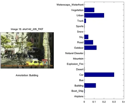
1.1 Class posterior probabilities of a scene annotated as Building . . 4

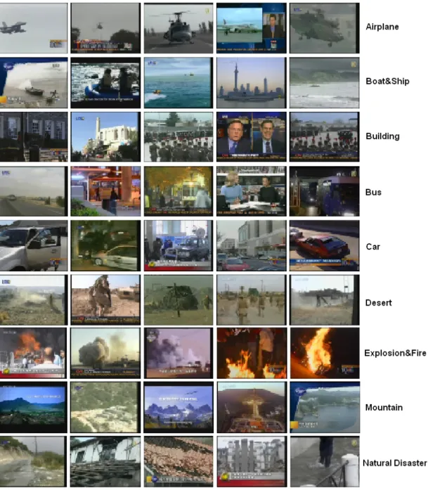
1.2 Example images from TRECVID dataset for classes Airplane, Boat&Ship, Building, Bus, Car, Desert, Explosion&Fire, Moun-tain, Natural Disaster. . . 6

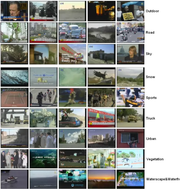
1.3 Example images from TRECVID dataset for classes Outdoor, Road, Sky, Snow, Sports, Truck, Urban, Vegetation, Water-scape&Waterfront. . . 7

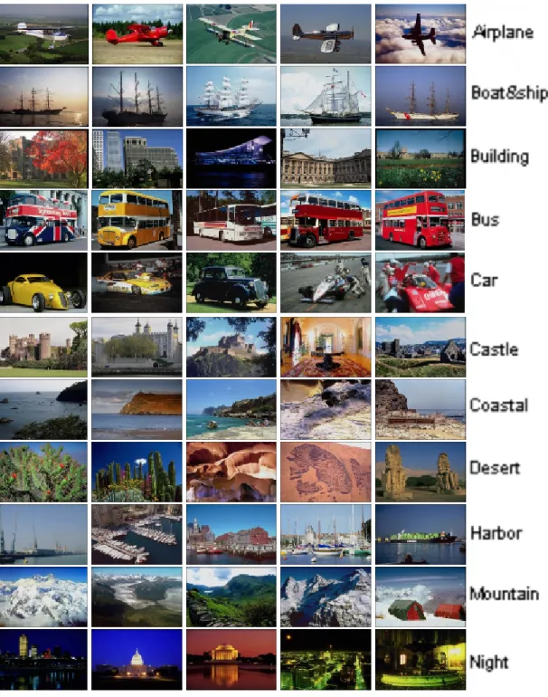
1.4 Example images from COREL dataset for classes Airplane, Boat&Ship, Building, Bus, Car, Castle, Coastal, Desert, Harbor, Mountain, Night. . . 9

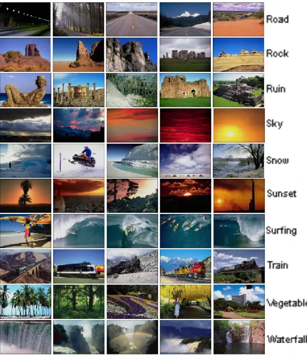
1.5 Example images from COREL dataset for classes Road, Rock, Ruin, Sky, Snow, Sunset, Surfing, Train, Vegetable, Waterfall. . . 10

3.1 Segmentation examples using spatial and spectral information: (a) Original images, (b) Results of segmentation process, (c) Results of filtering process . . . 20

4.1 Color pairs of two line segment groups ( Figure is taken from [15] ) 22

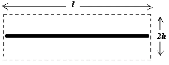
4.2 Rectangular region around a line segment with length l . . . 23

(10)

LIST OF FIGURES x

4.3 Determination of Number of Clusters in a Dendrogram . . . 25

4.4 Segmentation examples using line structure. First row: original images; second row: result of a color based line clustering; third row: Result of a position based line clustering within one of the color based clusters by average linkage (examples for good clus-ters); fourth row: Result of a position based line clustering within one of the color based clusters by average linkage (examples for bad clusters); fifth row: Result of a position based line clustering by single linkage; sixth row: Final result of line clustering; seventh row: Regions that are obtained from line clustering (outlier regions are showed with black color). . . 26

5.1 Class posterior probabilities of scenes for example images . . . . 36

6.1 Generation of a hyper-sphere to discriminate relevant images area by SVDD: Black circles denote relevant and gray boxes denotes the non-relevant images are evaluated by the user. Empty boxes are the displayed images that are not checked. ( Figure is taken from [21] ) . . . 39

6.2 Relevance Feedback Scenario . . . 40

7.1 Confusion matrices of TRECVID for two different models: (a) Confusion matrix for multi class classifier model, (b) Confusion matrix for one class model . . . 43

7.2 Mean average precision values (MAP) according to class poste-rior probabilities of each scene category of TRECVID dataset: (a) MAP values for multi class classifier model, (b) MAP values for one class classifier model. . . 45

(11)

LIST OF FIGURES xi

7.3 Precision vs. number of images retrieved plots of TRECVID for two different models. ‘Feedback 0’ refers to the retrieval without feedback: (a) Precision plot for multi class classifier model, (b) Precision plot for one class classifier model . . . 47

7.4 Mean average precision (MAP) graph of each scene category of TRECVID dataset for the original retrieval and the following 4 iterations. ‘Feedback 0’ refers to the retrieval without feedback: (a) MAP graph for multi class classifier model, (b) MAP graph for one class classifier model . . . 48

7.5 Confusion matrices of COREL for two different codebook types: (a) Confusion matrix for the codebook that is constructed by using HSV histograms of the regions, (b) Confusion matrix for the code-book that is constructed by using HSV and orientation histograms of the regions . . . 50

7.6 Mean average precision values (MAP) according to class poste-rior probabilities of each scene category of COREL dataset: (a) MAP values for the codebook that is constructed by using HSV histograms of the regions, (b) MAP values for the codebook that is constructed by using HSV and orientation histograms of the regions 51

7.7 Precision vs. number of images retrieved plots of COREL for two codebook types. ’Feedback 0’ refers to the retrieval without feed-back: (a) Precision plot for the codebook that is constructed by using HSV histograms of the regions, (b) Precision plot for the codebook that is constructed by using HSV and orientation his-tograms of the regions . . . 53

(12)

LIST OF FIGURES xii

7.8 Mean average precision (MAP) graph of each scene category of COREL dataset for the original retrieval and the following 4 iter-ations. ‘Feedback 0’ refers to the retrieval without feedback: (a) MAP graph for the codebook that is constructed by using HSV histograms of the regions, (b) MAP graph for the codebook that is constructed by using HSV and orientation histograms of the regions 54

7.9 Precision vs. number of images retrieved plots of COREL for bag of regions representation . . . 55

7.10 Mean average precision (MAP) graph of the original retrieval and the following 4 iterations for SVDD based and weight based back approaches. ‘Feedback 0’ refers to the retrieval without feed-back: (a) MAP graph for TRECVID dataset, (b) MAP graph for Corel dataset . . . 57

(13)

List of Tables

1.1 The number of training and testing images that are used for each class from TRECVID dataset . . . 5

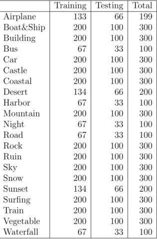
1.2 The number of training and testing images that are used for each class from COREL dataset . . . 8

7.1 Classification success rates for different k1 values for both multi

class classifier and one class classifier models . . . 42

(14)

Chapter 1 INTRODUCTION

1.1 Motivation

Content based image indexing and retrieval (CBIR) has become an extremely important issue with the use of large databases in a wide range of areas. Searching in huge image datasets according to their contents has been the major subject of many research areas in the last decade. Many studies are proposed for content-based analysis, indexing and retrieval in these types of datasets [11, 38, 4, 36, 34, 33, 27].

In CBIR, the image contents are represented by low-level features that are extracted from the images automatically by using several low-level feature ex-traction algorithms. Most of early approaches have resorted to global feature extraction to represent the images [13, 30, 9, 7, 31, 34, 33]. However the global features can not catch the semantic content of the images that humans receive. Hence the results of retrieval process may not satisfy the user.

In order to solve this problem, recent works propose techniques that uses local descriptors [10, 27] instead of global ones while indexing the images and include local information of the images in the model. Although these types of techniques have more advantages compared to global based ones, they are not successful

(15)

CHAPTER 1. INTRODUCTION 2

enough to model the visual content of the images.

The contextual information is very important to reflect the semantic content of the images. Having knowledge about the contextual information provides contribution to make more robust modeling while indexing the images since it reduces the gap between the low level features and high level content. As a result, more satisfied results to human perception is proposed in retrieval process.

Scene classification is a promising method to model the context in the images since it enables the images to be represented with semantic labels. Therefore, in indexing process of this work, scene classification techniques are used instead of direct local features representation to model the contextual information of the images. Each image is indexed with the probability of observing different semantic classes in it by using the classification results.This indexing structure is used in retrieval process to obtain more satisfactory results.

Scene classification is a difficult problem since determining context of an im-age depends not only on a single object in it as in object recognition. The context of an image is meaningful when consulting all entities in it. Therefore in order to model the scenes, the descriptors that represent all entities in the images should be used. Early approaches that only look global features extracted on the whole image [13, 30, 9, 7, 31, 34, 33] suffer from the incapability of the global features to derive higher semantic meanings of the images. Recent approaches use local descriptors in scene classification. The common characteristic of these approaches representing the images as histogram of local descriptors. They adapt the tra-ditional “bag of words” document analysis technique to the scene classification as “bag of visterms (visual terms)” [20, 17, 12, 35, 14, 25, 37]. The visual scene descriptors of the images stand for words in the documents here. Each image is modeled as a collection of local descriptors that come from the codebook con-structed. Most of the researches use invariant local descriptors called patches to represent the images [20, 17, 12, 14, 25]. However, using patches can give rise to visual polysemy problem since the same patches can be seen in different entities in the images. On this account, more meaningful descriptors for the scenes are used in this work. In order to achieve this, images are segmented into meaningful

(16)

regions by using color and line structure information of the images. By using the line structures of the images the regions that do not consist of uniform colors such as man made structures are captured. After all regions are clustered, each image is represented with the histogram of the region types it contains. Both multi-class and one-class classification models are used with these histograms to obtain the probability of observing different semantic classes in each image. Since a single class with the highest probability is not sufficient to model image content in an unconstrained data set with a large number of semantically overlapping classes, the obtained probability values are used as a new representation of the images and retrieval is performed on these new representations. For example in Figure 1.1 the graphic shows the probability values of observing different semantic classes in the image.

As seen in the Figure 1.1 the images that are used in the experiments can belong to more than one scene category semantically. While using the probability values in scene classification directly causes classification errors, using them in retrieval process that enables the contribution of each scene category gives more satisfactory results.

Although the probability based modeling reduces the gap between the simi-larities of the images in feature space and in the human perception, it can not eliminate the subjectivity of human perception. In order to overcome this prob-lem a relevance feedback technique is introduced and the user contribution is included to the retrieval process. According to user feedback the discriminant hyper-sphere is generated to represent relevant images area by using One Class Support Vector Data Description (SVDD) [32]. The images that are relevant to the user are ranked according to the discriminant hyper-sphere and displayed to the user. By this technique, retrieval performance is also increased in addition to its serving to the subjectivity of human perception.

(17)

(18)

1.2 Dataset

The performance of the proposed work is illustrated on two different datasets, TRECVID 2005 video shots and COREL dataset. Totally 24517 video shots that are manually labeled into 18 scene categories are used from TRECVID dataset. 16340 of them which are randomly selected from each class are used as training and remaining 8177 shots are used for testing processes. The number of video shots that are used for each class are shown in Table 1.1 with the names of the classes. Figure 1.2 and Figure 1.3 illustrate example shots from each class. Table 1.1 illustrates that the dataset contains semantically overlapping classes. As an example, the outdoor class covers almost all the classes.

Table 1.1: The number of training and testing images that are used for each class from TRECVID dataset

Training Testing Total

Airplane 54 27 81 Boat&Ship 53 27 80 Building 1333 667 2000 Bus 29 15 44 Car 419 210 629 Desert 136 68 204 Explosion&Fire 138 69 207 Mountain 91 46 137 Natural Disaster 47 24 71 Outdoor 6970 3485 10455 Road 550 276 826 Sky 2438 1220 3658 Snow 55 28 83 Sports 398 199 597 Truck 98 49 147 Urban 1527 764 2291 Vegetation 1740 870 2610 Waterscape&Waterfront 264 133 397 Total 16340 8177 24517

(19)

Figure 1.2: Example images from TRECVID dataset for classes Airplane, Boat&Ship, Building, Bus, Car, Desert, Explosion&Fire, Mountain, Natural Dis-aster.

(20)

Figure 1.3: Example images from TRECVID dataset for classes Outdoor, Road, Sky, Snow, Sports, Truck, Urban, Vegetation, Waterscape&Waterfront.

(21)

categories. Each category of scenes is randomly divided into two sets: 1663 for training and 1663 for testing. The number of images that are used for each scene category is listed in Table 1.2 and example sets for each category are illustrated in Figure 1.4 and Figure 1.5

Table 1.2: The number of training and testing images that are used for each class from COREL dataset

Training Testing Total Airplane 133 66 199 Boat&Ship 200 100 300 Building 200 100 300 Bus 67 33 100 Car 200 100 300 Castle 200 100 300 Coastal 200 100 300 Desert 134 66 200 Harbor 67 33 100 Mountain 200 100 300 Night 67 33 100 Road 67 33 100 Rock 200 100 300 Ruin 200 100 300 Sky 200 100 300 Snow 200 100 300 Sunset 134 66 200 Surfing 200 100 300 Train 200 100 300 Vegetable 200 100 300 Waterfall 67 33 100

1.3 Summary of Contribution

In CBIR, the image contents are often represented by low-level features that are extracted from the images automatically by using several low-level feature ex-traction algorithms. However low-level features are no longer sufficient for image

(22)

Figure 1.4: Example images from COREL dataset for classes Airplane, Boat&Ship, Building, Bus, Car, Castle, Coastal, Desert, Harbor, Mountain, Night.

(23)

Figure 1.5: Example images from COREL dataset for classes Road, Rock, Ruin, Sky, Snow, Sunset, Surfing, Train, Vegetable, Waterfall.

(24)

content representation. In this study each image is represented with the proba-bility of observing different semantic classes in it by using the scene classification techniques and retrieval is performed on these new representations. In order to minimize the semantic gap, a relevance feedback approach that is based on the support vector data description is also incorporated.

1.4 Organization of the Thesis

The organization of the thesis is as follows. Chapter 2 summarizes the related background work about annotation methods and relevance feedback techniques in content based image retrieval. Segmentation of images into regions by using spatial & spectral information and line structure information are described in Chapter 3 and Chapter 4 respectively. In Chapter 5, multi class and one class scene classifications that are used for indexing the images are presented. Chap-ter 6 introduces a CBIR framework with relevance a feedback technique that is based on one class support vector data description. Chapter 7 contains the ex-perimental results by applying our approaches to TRECVID and Corel datasets. We conclude with a discussion in Chapter 8.

(25)

Chapter 2 RELATED WORK

In the literature there are two main approaches in image retrieval according to image indexing method they use. First one is based on representation of the images by a set of keywords that are attached manually to images according to their contents. Queries are created using these keywords. Although efficient image indexing and access tools are available for annotating the images [39], these approaches are not preferable since image annotation is a tedious process. Firstly, it is a hard process to annotate all images of a huge database manually. Second, since a single image may include a multiplicity of contents, and since human perception and understanding vary it is almost impossible for the same images to be annotated with exactly the same keywords by different annotators. The second approach is more efficient than the first one. The images contents are represented by low-level features that are extracted from the images automatically by using several low-level feature extraction algorithms. Most of early approaches have resorted to global feature extraction to represent the images [13, 30, 9, 7, 31, 34, 33]. Vailaya [34] used color histogram, color coherence vector, DCT coefficient, edge direction histogram, and edge direction coherence vector as the features of the image in CBIR. However the global features can not be a solution for the semantic gap between the low level features of the images and high level contents of them. In order to achieve this problem, recent works propose two different types of techniques for CBIR. First one is using local descriptions [10, 27]

(26)

CHAPTER 2. RELATED WORK 13

instead of global ones while indexing the images and the other ones is using learning techniques [40, 8, 21, 4, 6, 23] in CBIR. Whereas Cordelia [27] used local invariant descriptors, Jing [10] used the segmented regions to represent the images. Since the descriptors they use are limited to model the context of the images, to use the performance of contextual information in CBIR many researches apply scene classification techniques to index the images with semantic class information [2, 38, 29, 16, 37]. Carneiro [2] used classification in order to annotate the images and perform retrieval based on this annotation. In order to annotate an image modeled by Gaussian mixture, he used minimum probability error rule based class densities obtained from Gaussian mixture models of images that are annotated with the same semantic class. In the SIMPLIcity system [38] the images are segmented and model-based approach is used to classify the images into basic classes. In CBIR, they used the features that are extracted from the segmented regions based on the classification results they performed. Smith and Li [29] proposed a scene classification method using composite region templates (CRTs) that are generated by using spatial ordering of segmented regions. Then they used classification information in order to index the images. Shapiro [16] used combination of multiple feature types that are extracted from the segmented regions. Multiple types of features are extracted by 3 different segmentation processes based on different context within an image. Then the combination of the features is used for annotation. Vogel [37] used the classification results to rank the images according to their semantic similarities to a semantic class.

When looking more deeply in scene classification recent works use “bag of visterms (visual terms)” technique in classification as mentioned in Chapter 1 [20, 17, 12, 35, 14, 25, 37]. Pedro [25] used difference of Gaussians (DOG) point detector to detect interest points which were used for generating invariant lo-cal descriptors. In order to generate patches (invariant lolo-cal descriptors) Per-ona [14] used 4 different ways: evenly sampled grid, random sampling, Kadir & Brady saliency detector, Lowe’s DOG detector. For recognition phase they used Bayesian hierarchical models for represent each class. Monay [20] used proba-bilistic aspect models in addition to “bag of visterms (visual terms)” approach

(27)

in order to solve the visual polysemy problem. Lazebnik [12] used spatial in-formation of the local descriptors addition to other approaches. She partitioned the images into sub-regions and computed the histogram of the patches inside in each sub-region. Marszalek [17] used spatial information of the patches in order to reduce the influence of the patches that come from the background by giving weights to patches. Gemert [35] and Vogel [37] divided the images in grid cells that are used as visual scene descriptors. Gemert [35] used overlapping grid cells as local descriptors. Gemert [35] thought that choosing a vocabulary to compose codebook is an inherent problem of codebook approach. Therefore in contrast to other approaches they used all vocabulary elements as a codebook.

Relevance feedback is a popular example for the second technique to narrow the gap between the low level features and high level concepts of the images. The typical scenario for relevance feedback in CBIR is as follows:

1. Initial retrieval results are displayed to the user.

2. User gives feedback to the system by selecting the images as relevant or irrel-evant according to his/her request.

3. System rearranges the results according to user feedback.

Step 1 and 2 is repeated iteratively until user is satisfied. Several relevance feedback algorithms are proposed in order to perform step 3. The traditional ones are based on assigning weights values to the low-level features and updating them according to the user feedback in CBIR [23, 26, 10]. Another approach called query point movement (QPM) tries to improve the results by moving the query point towards the relevant examples and away from the non-relevant examples [10, 6]. Jing [10] and Giacinto [6] uses Rocchio formula in order to improve the estimate of query point:

Q1 = α.Q0+ β.mR− γ.mN, (2.1)

where Q1 is the updated and Q0 is the original query, mR and mN means of

pos-itive and negative samples provided by user respectively. Rather than a redefin-ing a query, Cox [4] used Bayesian framework to estimate probability distribution over all images and update the distribution according to user feedback. The main

(28)

problem encountered by these approaches in relevance feedback is small feedback data provided by the user. Guo [8] and Setia [28, 8] tries to solve this problem by using support vector machines (SVM) which generate a discriminant hyper-plane that separates the relevant examples from the non-relevant ones. They updated the hyper-plane according to user feedback. Some researchers try to learn the boundary from only relevant or irrelevant samples and use one class SVM instead of two class [21, 3].

(29)

Chapter 3 SEGMENTATION USING

COLOR INFORMATION

Scene classification is a difficult problem since determining context of an image depends not only on a single object in it as in object recognition. The context of an image is meaningful when consulting all entities in it. Therefore in order to model the scene of the images the descriptors that represent all entities in the images should be used. Early approaches that only look global features extracted on the whole image [13, 30, 9, 7, 31, 34, 33] suffer from the incapability of the global features to derive higher semantic meanings of the images.

In scene classification phase of this work, “bag of visterm” technique [20, 17, 12, 35, 14, 25, 37], which models the images as a collection of visual scene descriptors, is used. Using invariant local descriptors (patches) [20, 17, 12, 14, 25] as visterms can give rise to visual polysemy problem since the same visterms can be seen in different entities in the images. On this account, more meaningful descriptors for the scenes are used in this work. In order to achieve this, images are segmented into meaningful regions.

Image segmentation is still an unsolved problem in image processing and com-puter vision. The images that include fewer number of objects in a simple back-ground can be segmented successfully by recent studies. However, estimating

(30)

CHAPTER 3. SEGMENTATION USING COLOR INFORMATION 17

common set of parameters makes these studies deficient for large and complex image datasets. Another problem for common segmentation algorithms is using only spectral information of the images. Performing segmentation process only in spectral domain causes noisy structure in the images. Therefore spatial infor-mation is also used in addition to spectral inforinfor-mation in our approach. In the spectral domain, HSV color values and in the spatial domain position values of the corresponding image pixels are used and these two types of information is combined by combined classifier approach [22].

In the first step of the segmentation, an initial labeling process is performed for the image pixels and a labeled pixel dataset is constructed for each image. After initial labeling step, a new labeling is started iteratively.

The initial labeling is performed by k-means clustering algorithm in spec-tral (HSV color values) domain and each pixel is assigned to a cluster t, where t = 1, . . . , T . The next labeling step of the initially labeled pixels is performed by using both spectral (HSV color values) and spatial (position values) infor-mation. In this step, nearest mean classifier is trained on the spectral domain and Parzen classifier with Gaussian kernel is trained on the spatial domain it-eratively. By running the trained classifiers on the same datasets, two class posterior probabilities are computed for each pixel of the image. Pspec(wt|xi) and

Pspat(wt|x0i), t = 1, . . . , T . xi is 3 dimensional feature vector that contains HSV

values and x0_i is 2 dimensional feature vector that contains x and y coordinates of the pixel i. For assigning a new label to each pixel both probability values are combined by using the product combination rule:

R is number of pixels in each image. New class label that maximizes the combi-nation probability Pcomb(wt|xi) is assigned to the pixel i.

This new labeling process is an iterative procedure. At each iteration, the results of spectral and spatial classifiers are combined and new labels are assigned to the pixels by combined classifier until a stable segmentation is reached before

(31)

20 iterations. Assume that the label of pixel i at iteration j is λij, j ≥ 0. Then

lets define a function DIF Fj,j+1 that gives number of labels changes between the

iterations j and j + 1. DIF Fj,j+1 = R X i=1 I(λij, λij+1) (3.2)

where I is the indicator function:

I(λa, λb) =

(

1 λa6= λb

0 otherwise (3.3)

A stable segmentation is reached if DIF Fj,j+1 = 0 for two consecutive

itera-tions j and j + 1. The labels of the pixels in the 20th iteration are used if a stable segmentation has not been reached yet.

In most segmentation algorithms the number of regions have to be predefined. However estimating a region number that is suitable for all images in a dataset is considerably hard issue. By using combined classifier approach dynamic region number is attained for each image since after segmentation process there are regions that share same class labels but are located in different locations in the image. Hence, the only parameter that has to be estimated is an approximate value for number of dominant colors, T , which is common for all images.

Since many inhomogeneous color regions are available as well as smooth ones, after segmentation process the segmented images can have many noisy pixels as seen in the second column of the Figure 3.1. In order to eliminate these noisy pixels, a two step filtering process is performed on segmented images. In the first step, the segmented regions that are smaller than a threshold, F , are eliminated and labeled as outlier. In the second step, the regions that are labeled as outlier and smaller than a threshold, B, are merged to their closest neighbor regions. Examples for segmentation and two step filtering processes are shown in Figure 3.1. The original images are given in the first column. The second column shows the segmentation results before applying filtering process. After filtering, the final segmentation results are shown in the last column. The black

(32)

regions denote the regions that are labeled as outlier. As seen, the regions are captured by this segmentation process are color uniform regions. The entities with miscellaneous colors are eliminated as outlier regions. These types of regions are captured by using their line structural information as explained in the next chapter.

(33)

(a) (b) (c)

Figure 3.1: Segmentation examples using spatial and spectral information: (a) Original images, (b) Results of segmentation process, (c) Results of filtering pro-cess

(34)

Chapter 4 SEGMENTATION USING LINE

STRUCTURE

Some objects that do not consist of uniform colors can not be segmented by using basically color information of the pixels. The edge structure of the man made ob-jects that includes miscellaneous colors are more distinct feature rather than the color information for them. They generally consist of regular line segments that share common color pairs from two sides (Figure 4.1). In this work, segmentation process is performed by using color information around line segments and the line segments that share common color pairs from two sides are grouped. Since dif-ferent objects that are close to each other may consist of common colors, their line segments can be located in the same line group.Therefore, presegmented re-gions are segmented again by using the position information of the line segments. In order to perform segmentation processes hierarchical clustering algorithm is used since constructing hierarchical structure on the line segments allows us to use dynamic number of regions. By deciding the cutting level of the hierarchical structure, suitable number of regions for each image can be estimated.

(35)

CHAPTER 4. SEGMENTATION USING LINE STRUCTURE 22

Figure 4.1: Color pairs of two line segment groups ( Figure is taken from [15] )

4.1 Extracting Line Features

First the edges from the images are extracted by using canny edge detector [1]. Then object recognition tool (ORT) line detector is applied to extracted edges in order to get line segments [5]. The jth_{line segment, L}

ij extracted from the image

Ii is represented as a feature set with 5 values:

Lij = { sx, sy, ex, ey, l } i = 1, . . . , n j = 1, . . . , m (4.1)

Above, n stands for the number images in the dataset and m stands for the number of line segments in image Ii. sx, sy and ex, ey are x and y coordinates of

the start and end points of the line segment Lij respectively. Length of Lij is l.

The color information around the line segments that belong to same object are expected to be similar. The line segments of an object usually contain two major colors around them as can be seen in the example in Figure 4.1. Both buildings have two observable colors. One comes from the windows and the other one comes from concrete of the buildings. If we imagine them as line structures we realize that the line segments that belong to same building share two common color pairs one from one side, the other one from other side. Therefore we can say that color information of the line segments is a distinguishing feature for the

(36)

objects (e.g. man made structures) with regular line segments and miscellaneous colors. This information can be used to segment the images that contain this type of objects into meaningful regions. In order to perform segmentation, first the average RGB color values for defined rectangular regions that cover the line segments are calculated. An example for a rectangular region that covers a line segment with length l is shown in Figure 4.2. It has 2h units height.

Figure 4.2: Rectangular region around a line segment with length l

Average RGB color values are calculated for two sides of the line segment separately. Therefore, each line segment is represented by 6 color values; 3 of them come from the left and the other 3 come from the right region of the rectangle.

These 6 color values are appended to the previous line feature set Eq. 4.1 and each line segment is represented with new feature set as follows:

Lij = { sx, sy, ex, ey, l, Rr, Gr, Br, Rl, Gl, Bl } i = 1, . . . , n j = 1, . . . , m

(4.2) Rr, Gr and Br are the average RGB values on the right and Rl, Gl and Bl are

the average RGB values on the left region of the line Lij.

4.2 Clustering Line Segments

In order to detect the regions that include common line structure, first the line segments in each image are clustered according to their color pairs (Section 4.2.2). In the second phase, position based clustering is performed within the preclus-tered line segments in order to separate different objects which are close to each other and share common line color pairs (Section 4.2.3). In order to estimate an

(37)

optimal number of regions for each image, stopping rule technique of hierarchical clustering is used (Section 4.2.1).

4.2.1 Determining Number of Clusters

The main problem in clustering is to decide the number of clusters because the number of objects in an image varies according to the image complexity. Stop-ping rule for hierarchical clustering is used to estimate an optimum number of clusters for each image [19]. This rule is based on the determination of the cutting level of the dendrogram that is created by agglomerative hierarchical clustering. The dissimilarity matrix of line segments for each image is calculated by using Euclidean distance measurement. Then for each image a dendrogram is created as a result of agglomerative hierarchical clustering. The problem is at which level the dendrogram is cut and which partitions are used as clusters. For example in the Figure 4.3, if the dendrogram is cut at the level between 4 and 5 where the cutting dissimilarity value is 45 then the resulted cluster number is 4. The question is why it is 45. Assume that we have m line segments in image Ii. Then

number of levels in the created dendrogram is m − 2. The stopping rule uses the distribution of the dissimilarity values that are used for creation of the dendro-gram at each level. The most appropriate level to cut the dendrodendro-gram is the first level j that satisfies:

αj+1 > α + bsα j = 1, . . . , m − 2 (4.3)

where αj+1 represents the distance between the partitions at level j + 1; α is the

mean and sα is the unbiased standard deviation of the α distribution; b is the

standard deviate which is a threshold that determines how many sα units the α

value deviates from the mean, α. After determining the cutting level j, optimum number of clusters is calculated as m − j.

(38)

Figure 4.3: Determination of Number of Clusters in a Dendrogram

4.2.2 Clustering According to Color Information

As mentioned the color information around the line segments that belong to same object are expected to be similar. Therefore, the first clustering is performed according to color information of the line segments by using average linkage hier-archical clustering. Using single or complete linkage in clustering can cause some dissimilar clusters to merge due to the outliers they contain. However in average linkage clustering this situation does not occur since each cluster is represented with its average of its members.

By using Euclidean distance measurement, dissimilarity matrix of line seg-ments in each image for hierarchical clustering is calculated. In this calculation 6 color values, Rr, Gr, Br, Rl, Gl, Bl, of the line segments from the feature set

Eq. 4.2. Line segments in each image are clustered into an optimum number of clusters that is estimated by the stopping rule of hierarchical clustering as mentioned in Section 4.2.1. The second row of Figure 4.4 shows some examples for clustered lines according to their color pairs (Clusters are shown with unique colored lines).

(39)

Figure 4.4: Segmentation examples using line structure. First row: original im-ages; second row: result of a color based line clustering; third row: Result of a position based line clustering within one of the color based clusters by average linkage (examples for good clusters); fourth row: Result of a position based line clustering within one of the color based clusters by average linkage (examples for bad clusters); fifth row: Result of a position based line clustering by single linkage; sixth row: Final result of line clustering; seventh row: Regions that are obtained from line clustering (outlier regions are showed with black color).

(40)

4.2.3 Clustering According to Position Information

In outdoor images, many different objects have lines with similar color values. As seen in the examples at the second row of Figure 4.4, the lines segments of different entities may still belong to the same clusters. For the first and second example images, the lines of two different buildings belong to the same clusters. In the third example image, it is valid for the lawn part. To rule out such situations, position information of line segments are used. Within the color based line segments they are clustered according to their position information, first using average linkage then single linkage hierarchical clustering algorithms.

4.2.3.1 Step1: Average Linkage Hierarchical Clustering

In order to cluster line segments according to their positions first average linkage hierarchical clustering is used. Average linkage is preferred to reduce the outlier effects of the clusters. To calculate the distance matrix of the line segments both their start and end points are used.

D =             d11 d12 . . . d1m d21 d22 ... d2m . . . . . . . . . . . . dm1 dm2 . . . dmm             dij = min{d(si, sj), d(ei, ej)} i, j = 1, .., m (4.4)

si is the start point with the coordinates six and siy, ei is the end point with

the coordinates eix and eiy of the ith line segment. D is m by m distance matrix

of the line segments that are in the same color based cluster. dij stands for the

distance between the ith _{and j}th _{line segments and take the value of minimum of}

d(si, sj) and d(ei, ej). d(si, sj) and d(ei, ej) are Euclidean distances of the start

(41)

After calculating the distance matrix within the color based line segments, clustering is performed by using average linkage hierarchical clustering. Some clusters have a few number of line segments that can not be appropriate to form an object. Therefore some clusters have less than 3 line segments are discarded as a result of elimination process. Third row of the Figure 4.4 shows the results of the position based clustering within one of the color based clusters for each sample image.

Although some resulted clusters have adequate line segments to form an ob-ject, their line segments can be too scattered and not exhibit a compact form. These type of line segments usually occur in the boundaries of the objects since the boundary lines share common color pairs one comes from outside, the other from inside of the object. In Figure 4.4, these types of clusters for the sample images can be seen. To rule out this problem a criteria that gives acceptability rate for a cluster is introduced. This criteria is based on the organization of the line segments. If line segments in a cluster exhibit a compact form then this cluster is a good cluster, otherwise, if the line segments exhibit a scattered form then the cluster is a bad cluster. A ratio for each cluster is defined in order to determine this criteria.

Riv =

Aiv

Miv

(4.5) where v is cluster id in image Ii; Aiv is the area of convex hull that includes all

line segments in cluster v; Miv is the number of lines in cluster v. If Riv > 450

then the cluster v is not acceptable to represent an object or a region in the image. After applying average linkage hierarchical clustering, the clusters whose Riv ratio is bigger than 450 are eliminated and the next steps are not performed

for these clusters. If Riv <= 100 then the cluster v is a good cluster. After

applying average linkage hierarchical clustering the clusters whose Riv ratio is

smaller than or equal to 100 are accepted and the next steps are not performed for these clusters.

(42)

4.2.3.2 Step3: Single Linkage Hierarchical Clustering

Sometimes the optimal number of clusters estimated by stopping rule is inade-quate to divide line clusters to get the best region representations. Some clusters still have some irrelevant line segments because of color similarity. The form of the clusters are distorted by these irrelevant line segments. This type of clusters are neither in the bad category nor the good one. Their Riv ratio is between

100 and 450 and should be clustered again. Therefore the line segments in these clusters are clustered by single linkage hierarchical clustering. Single linkage sim-ilarity method is used this time since the main purpose here is eliminating the outlier lines from the clusters. In the third row of Figure 4.4, the green line segments, which belong to two different buildings exhibit this like of destructed forms. At the fifth row of the Figure 4.4, the results of reclustering step for this cluster can be seen.

The final results of line based segmentation process are shown at the sixth row of the Figure 4.4 for the sample images.

4.3 Representing Line Segment Clusters as

Re-gions

Each line segment cluster represents a region for an image. Segmentation of the images with respect to these line segment clusters is a challenging topic. The first idea that comes to mind is, defining convex hulls which cover all line members of each cluster. However, it causes using of irrelevant area with meaningful regions due to the concave hull structure of the clusters. To rule out this problem a more appropriate method that preserves the form of clusters is introduced. First the images are partitioned into non-overlapping grid cells. Then each grid cell is labeled with the label of the cluster any of whose line member makes an inter-section with the corresponding cell. If there is no interinter-section or the number of intersections in grid cell does not reach a sufficient value then the corresponding cell is labeled as outlier. Finally each line cluster is represented by grid cells as

(43)

seen at the last row of the Figure 4.4.

Bu using the line structure information of the images, the regions, which are eliminated with color based segmentation process (Chapter 3), are captured. Therefore the meaningful regions, which do not consist of uniform colors and are labeled as outliers are captured in the line structure based segmentation process.

(44)

Chapter 5 SCENE CLASSIFICATION

Scene classification is a different research area from the object categorization since in scene classification, determining scene of an image does not depend on fixed content as in object categorization. Contents of an image that belongs to a specific scene can vary. This varied content of the scenes gets scene classification into more challenging problem and the techniques that are used in object categorization can not be used in scene classification. In order to model the scene of an image, visual components that are large enough to represent all entities in the image should be used. Recent approaches use local descriptors as visual components in scene classification. The common characteristic of these approaches is adapting the traditional bag of words document analysis technique to the scene classification as bag of visterms [24, 18, 20, 17, 12, 35, 14, 25]. The visual scene descriptors of the images stand for words in the documents here. Each image is modeled as a collection of local descriptors that come from the codebook constructed. Most of the researches use invariant local descriptors called patches to represent the images [20, 17, 12, 14, 25]. However, using patches can give rise to visual polysemy problem since the same patches can be seen in different entities in the images. On this account, more meaningful descriptors that are obtained as a result of the segmentation process (Chapter 3, Chapter 4) are used in this work.

Another popular problem encountered in scene classification is the restriction of number of classes. Many approaches use limited number of classes in their

(45)

CHAPTER 5. SCENE CLASSIFICATION 32

studies and most of them restrict their studies to two class classification problem. The performed work has dealt with large number of classes. In both datasets, TRECVID and Corel include large number of scene categories. In the following sections the steps in our scene classification algorithm are described.

5.1 Image Representation

The images are represented as a collection of regions that come from the con-structed region codebooks.

5.1.1 Region Codebook Construction

In our work two different types of regions are used, one of them comes from color based segmentation and the other one comes from line based segmentation process. Each of these two region collections are represented by different ways and a region codebook is constructed for each of them.

5.1.1.1 Codebook Construction Using Color Based Segmented Re-gions

The regions which are extracted by color based segmentation process explained in Section 3 are modeled using the multivariate histogram of the HSV values with 8 bins used for the H channel and 3 bins for each of S and V channels, resulting in a 72-dimensional features vector. Then the codebook for k1 region clusters are

learned by performing k-means algorithm on the region features.

5.1.1.2 Codebook Construction Using Line Segment Clusters

Two different representations for line segment clusters are used. One of them is same as the color based region representations. The regions that are obtained

(46)

by grid cells method explained in Section 4.3 are modeled by HSV histograms as described above (Section 5.1.1.1). The other representation method is based on orientation values of line segment clusters since the color values in a line based region may not be stable. Each line segment cluster is modeled using 10-bin histogram of orientation values of its line segments. These two types of representations are used separately in our work. After the regions are modeled for line clusters, the codebook for k2 region types is obtained by applying k-means

algorithm on the region features.

The codebooks that are generated as a result of two different region types are combined and a new codebook with k1+ k2 region clusters are constructed.

5.1.2 Image Features

After region codebook is constructed and k1 + k2 region types are determined,

each image is represented as a bag-of-regions as below by calculating histogram of the region types it contains.

Ii = {ri1, . . . , rit} (5.1)

where {ri1, . . . , rit} are the regions the image Iicontains and t denotes the number

of regions in image Ii.

5.2 Classification

For probability estimation two different classification models are used: multi class and one class. In both settings, the goal is to estimate the posterior probabilities P (wj|r1, . . . , rt), j = 1, . . . , c, where wj represents the jth class, c is the number

(47)

5.2.1 Multi Class Scene Classification

The images are classified using the Bayesian decision rule according to posterior probabilities. The image with the set of regions {r1, . . . , rt} is assigned to the

class

w∗_j = arg max

j=1,...,cp(wj|r1, . . . , rt) (5.2)

where wj represents the jth class, c is the number of classes, and t is the number

of regions in the scene. Using the Bayes rule, the posterior probabilities can be computed as

P (wj|r1, . . . , rt) =

P (r1, . . . , rt|wj)P (wj)

P (r1, . . . , rt)

. (5.3)

Assuming equal priors for all classes, the classification problem reduces to the computation of class-conditional probabilities P (r1, . . . , rt|wj).

Each region is assumed to be independent of others given the class. Therefore class conditional probability can be calculated as

P (r1, . . . , rt|wj) = t

Y

i=1

P (ri|wj). (5.4)

The probability of region ri having label u is computed as

P (ri = u|wj) = Pju =

nju

nj

. (5.5)

where u ∈ 1, . . . , k1+ k2 , j = 1, . . . , c, nju is the number of regions with the

label u in the training set for class j, and nj is the total number of regions in the

training set for class j.

5.2.2 One Class Scene Classification

Since the scene classes may not be mutually exclusive, the multi class classification is not always suitable. Therefore one class classification has also been used and each class is independently modeled. Assuming all classes in the training set form a normal distribution, classifiers that estimate a Gaussian density on each

(48)

class are trained. Therefore probability density function for the jth _{class can be}

calculated from the following equation:

P (x|wj) = 1 (2π)d2(Σ_j) 1 2 e−12 (x−µj) T_(Σ j)−1(x−µj) _(5.6)

where x is the histogram vector of region types with length k1+ k2 for an image in

jth_{class, µ}

j and Σj are the mean and covariance matrix of the jthclass. These are

estimated from the training samples. The test images can be classified according to posterior probabilities

P (wj|x), j = 1, . . . , c (5.7)

and again from the Bayes rule, assuming equal priors for all classes, the classifi-cation problem reduces to P (x|wj).

The images that are used in the experiments can belong to more than one scene category semantically. For instance, the example images in Figure 5.1 can not belong to exactly one scene category. The graphical representations of the class probability values of each image are shown on the top.

As seen in the Figure 5.1 the probability values for the scenes that images can belong to are similar to each other. Whereas assigning the first two images to the scene categories with the maximum probability gives successful results, for the last two images, using probability values results in failure in classification. For example the third image which is annotated as Boat&Ship, will be labeled as WaterScape&Waterfront in classification process, although the probability of belonging to Boat&Ship class is high.

Therefore instead of assigning strict labels to the images, they have been modeled with their class posterior probabilities and the models are used as indices of the images in retrieval process. Thanks to this method, contribution of each scene category can be used for representing the images.

(49)

(50)

Chapter 6 CONTENT BASED IMAGE

RETRIEVAL WITH

RELEVANCE FEEDBACK

In content based image retrieval there is always a gap between the high level semantics of the images that human perceives and the low level features of the images that machines compute. In order to deal with the semantic gap prob-lem various relevance feedback algorithms are proposed in the area of content based image retrieval and include the user in retrieval process. In most com-mon techniques, user judges the retrieved results as relevant or non-relevant to the query image. Then new results are calculated by using the feedback of the user. The user applies feedback until getting satisfactory results. There are var-ious algorithms for recalculation of new results according to user feedback. The main problem encountered in relevance feedback approaches is small feedback data provided by the user. Some approaches tries to solve problem by using classification techniques. One of the most popular techniques is using support vector machines (SVM) which generate a discriminant hyper-plane that separate the relevant examples from the non-relevant ones [28, 8]. Then the images that are in the relevant side are reranked according to distance to the hyper-plane in descending order. The major stumble in this approach is treating the problem as

(51)

CHAPTER 6. CONTENT BASED IMAGE RETRIEVAL WITH RELEVANCE FEEDBACK38

two class classification problem. It is straightforward to assume that all relevant images belong to the same class. On the other hand, the classes of non-relevant images probably vary. Hence forcing to assign them to the same class decreases the retrieval performance. In this work, to deal with this problem a relevance feedback approach is proposed by using one class data description technique, Support Vector Data Description (SVDD) [32, 21]. One class SVDD is inspired by Support Vector Classifier and can be used for classification where one of the classes is sampled well and the other one is not. SVDD generates a discrimi-nant hyper-sphere that can separate the target class from the outliers. Detailed description about SVDD is explained in Appendix A.

In our work, the relevant images that user presents are used as target samples and non-relevant images as outliers. While SVDD tries to find a hyper-sphere which contains most of the target samples, by using non-relevant samples it tries to minimize the volume of the sphere in order not to include any superfluous space. Therefore, it uses also outliers to find a more efficient description [32].

In retrieval scenario, using region histogram features as image features is not an effective way to represent the images since the number of region types that an image includes is very small related to the total number of region types. Therefore, the images are modeled with class posterior probability values that come from classification process for each class.

In the first retrieval process, the images are sorted according to the poste-rior probability values of the scene class that user searches for and displayed to the user. After obtaining a feedback from the user an optimum hyper-sphere is generated by SVDD that separates the relevant samples from the non-relevant ones. Then again the images in the relevant area are ranked in decreasing order according to the distance to the hyper-sphere. After the images in non-relevant area are ranked in increasing order according to the distance to the hyper-sphere, they are appended to the first ranking group (Figure 6.1). Then the results are shown to the user to obtain a new feedback until a satisfactory result is reached. Whole retrieval scenario with relevance feedback is shown in Figure 6.2.

(52)

Figure 6.1: Generation of a hyper-sphere to discriminate relevant images area by SVDD: Black circles denote relevant and gray boxes denotes the non-relevant images are evaluated by the user. Empty boxes are the displayed images that are not checked. ( Figure is taken from [21] )

overlapping since by giving the individual contribution, the user eliminates the visual polysemy in his/her point of view.

(53)

(54)

Chapter 7 EXPERIMENTS

7.1 TRECVID

7.1.1 Classification

A codebook has been learned from the regions that are extracted from whole dataset by a segmentation process. Because of crowded and complex structure of the images in TRECVID dataset, line based segmentation process gives bad performance on this dataset. Therefore, the segmentation has been performed by using only color information (Chapter 3). The values of 5, 7 and 10 are used for T . The value 7 has been selected for T as a result of observations on a randomly selected sample dataset. The elimination process, which is the last part of segmentation, is performed by using values 2000 for F and 100 for B. The codebook is constructed from the regions that are modeled by HSV color histograms by using the values 100, 500 and 1000 for k1. Two type of models

for each category of scenes have been obtained from the training images. One of the models is created by using multi class classifier and the other is created by using one class classifier that fits Gaussian model on each class independently. One class classifier has been used in order to eliminate classification errors arise from class overlapping problem. The value 1000 for k1 gave the best classification

(55)

CHAPTER 7. EXPERIMENTS 42

results for both model types as seen in Table 7.1.

Table 7.1: Classification success rates for different k1 values for both multi class

classifier and one class classifier models

Multi Class One Class k1 = 50 %18 %13

k1 = 200 %25 %12

k1 = 500 %32 %10

k1 = 1000 %38 %10

Confusion matrices for classification result are illustrated in Figure 7.1 for both types of models. On the confusion matrices each column represents the instances in the predicted class and each row represents the instances in an actual class. Overall classification accuracies are 16.57% and 10.26% for Figure 7.1(a) and Figure 7.1(b), respectively.

The low performance for multi class classification is obtained for “outdoor” and “sky” classes as seen in the confusion matrix in Figure 7.1. These are the expected results for the scene categories that enclose other scenes semantically. Most of the images in TRECVID dataset are outdoor images and include sky scene. There is also class overlapping problem for all other scene categories. Ne-cessity of assigning each image, which can belong to multiple scene categories but annotated with one of them, to a single class reduces the success rates dra-matically. The last two images in the Figure 5.1 of Chapter 5 is an evidence of this situation. The third image, which is annotated as Boat&Ship, is predicted as WaterScape&Waterfront in classification process since it should be assigned to the class with the maximum probability. Since “outdoor” is more general scene category, in one class model there is also instability problem for the number of class instances. Number of instances in the “outdoor” class exceeds all other class populations. Therefore, the Gaussian model for the “outdoor” class encap-sulates most of the images in other classes. Although it is an expected situation, it raises problems in classification process. As seen in confusion matrix in Fig-ure 7.1(b) most of the images in different categories are predicted as “outdoor”

(56)

(a)

(b)

Figure 7.1: Confusion matrices of TRECVID for two different models: (a) Con-fusion matrix for multi class classifier model, (b) ConCon-fusion matrix for one class model

(57)

since TRECVID dataset consists of outdoor images. In confusion matrix, the other scene category dominates others is “sky”. It is an expected situation since most of outdoor images include sky but the results are reflected as classification errors.

In order to show the performance of probability model we sort the images according to class probabilities for each category then we calculate mean average precision (MAP) values using this ranking (Figure 7.2). For multi class classifi-cation model (Figure 7.2(a)), MAP values are above 0.5 for all classes. As seen in Figure 7.2(a) and Figure 7.2(b), the performances of both multi class and one class models are very high for “outdoor” and “sky” classes.

7.1.2 Retrieval with Relevance Feedback

Instead of using class probabilities obtained from classification process, they are used for image representation in a retrieval process. Each image is represented by a vector whose components are class posterior probabilities for each scene category. The classification results are used for generating queries automatically and ground truth is used for providing feedback to the system. Quarter of the images of each class population is used as query images. For each query, the top 30 images are employed for providing feedback by automatically labeling each image that belonged to the same ground truth group with the query as relevant and the remaining images as irrelevant at each iteration. This process is repeated for each selected query image for 4 feedback iterations. Figure 7.3 shows precision plots of the original retrieval and the following 4 iterations for multi class and one class classifier models. Figure 7.4 illustrates the mean average precision values (MAP) of each scene category again for multi class and one class classifier models. MAP values are calculated for the original retrieval and the following 4 iterations. For both of the models the first iteration gave the largest increase in precision. A little rise is obtained for the next 4 iterations. The precision values for one class classification model is much higher than the multi class classification model since while calculating the posterior class probabilities for overlapping classes, learning a boundary for each class that separates it from

(58)

(a)

(b)

Figure 7.2: Mean average precision values (MAP) according to class posterior probabilities of each scene category of TRECVID dataset: (a) MAP values for multi class classifier model, (b) MAP values for one class classifier model.

(59)

the others is more efficient than learning a boundary that separates all the classes from each other. In TRECVID dataset the big problem is existence of “outdoor” class. It is almost impossible to represent the “outdoor” scene category with multinomial model since it can not be separated from the other classes. Both results are more acceptable than the classification results since the contribution of each of 18 scene categories are used in image representations. Since high precision values have been already reached in the first retrieval, satisfactory increases can not be obtained for feedback iterations. TRECVID dataset is a hard dataset for classification. Images in TRECVID dataset have complex background with multiple contents and it is not possible to assign them to a single class. In order to retrieve more realistic performance, we annotate the images with multiple class labels to use in retrieval process. While calculating the precision values, we use all possible class labels of the images. This is the main reason that the retrieval performance is higher than the performance of COREL dataset which will be explained in the next Section 7.2.

7.2 COREL

7.2.1 Classification

For COREL dataset the codebook is generated by using the regions that are ob-tained by both color based and line based segmentation processes. The value of 1.6l is used for h, to create the rectangle that surrounds a line segment which has a length l. In order to determine the the number of line clusters, stopping rule is applied to the line clustering using the value 4 for b. The color based segmentation and elimination processes are performed with the same parameters as the parameters that are used in TRECVID dataset. Two types of codebooks are constructed from the color based and line based regions. The regions from the codebook, which is obtained by the color based segmentation, are modeled by HSV color histograms. Region clustering uses 1000 for k1. The regions from the

(60)

(a)

(b)

Figure 7.3: Precision vs. number of images retrieved plots of TRECVID for two different models. ‘Feedback 0’ refers to the retrieval without feedback: (a) Precision plot for multi class classifier model, (b) Precision plot for one class classifier model