a thesis
submitted to the department of computer engineering
and the graduate school of engineering and science
of bilkent university
in partial fulfillment of the requirements
for the degree of
master of science
By
Erdem ¨
Ozdemir
August, 2011
I certify that I have read this thesis and that in my opinion it is fully adequate, in scope and in quality, as a thesis for the degree of Master of Science.
Assist. Prof. Dr. C¸ i˘gdem G¨und¨uz Demir (Advisor)
I certify that I have read this thesis and that in my opinion it is fully adequate, in scope and in quality, as a thesis for the degree of Master of Science.
Prof. Dr. Cevdet Aykanat
I certify that I have read this thesis and that in my opinion it is fully adequate, in scope and in quality, as a thesis for the degree of Master of Science.
Prof. Dr. Fato¸s Yarman Vural
Approved for the Graduate School of Engineering and Science:
Prof. Dr. Levent Onural Director of the Graduate School
FOR AUTOMATED CANCER DIAGNOSIS
Erdem ¨Ozdemir
M.S. in Computer Engineering
Supervisor: Assist. Prof. Dr. C¸ i˘gdem G¨und¨uz Demir August, 2011
Correct diagnosis and grading of cancer is very crucial for planning an effective treatment. However, cancer diagnosis on biopsy images involves visual interpreta-tion of a pathologist, which is highly subjective. This subjectivity may, however, lead to selecting suboptimal treatment plans. In order to circumvent this prob-lem, it has been proposed to use automatic diagnosis and grading systems that help decrease the subjectivity levels by providing quantitative measures. How-ever, one major challenge for designing these systems is the existence of high variance observed in the biopsy images due to the nature of biopsies. Thus, for successful classifications of unseen images, these systems should be trained with a large number of labeled images. However, most of the training sets in this domain have limited size of labeled data since it is quite difficult to collect and label histopathological images. In this thesis, we successfully address this issue by presenting a new resampling framework. This framework relies on increasing the generalization capacity of a classifier by augmenting the size and variation in the training set. To this end, we generate multiple sequences from an image, each of which corresponds to a perturbed sample of the image. Each perturbed sample characterizes different parts of the image, and hence, they are slightly different from each other. The use of these perturbed samples for representing the image increases the size and variability of the training set. These samples are modeled with Markov processes which are used to classify unseen image. Work-ing with histopathological tissue images, our experiments demonstrate that the proposed framework is more effective for both larger and smaller training sets compared against other approaches. Additionally, they show that the use of per-turbed samples is effective in a voting scheme which boosts the performance of the classifier.
iv
Keywords: Histopathological image analysis, automated cancer diagnosis, resam-pling, Markov models, cancer.
¨
ORNEKLEME BAZLI MARKOV MODELLEME
Erdem ¨Ozdemir
Bilgisayar M¨uhendisli˘gi, Y¨uksek Lisans
Tez Y¨oneticisi: Yar. Do¸c. Dr. C¸ i˘gdem G¨und¨uz Demir August, 2011
Do˘gru kanser tanısı ve derecelendirilmesi, etkili bir tedavi planı i¸cin ¨onemlidir. Ancak, biyopsi g¨or¨unt¨uleri ¨uzerinde yapılan kanser tanısı, patologların g¨orsel olarak yorumlamasına dayanır, bu ise ¨oznellik ta¸sır. Bu ¨oznellik, etkili ol-mayan tedavi planlarının uygulanmasına yol a¸cabilir. Tanıdaki ¨oznelli˘gi azaltmak amacıyla, ¨ol¸c¨ulebilir de˘gerler ¨uzerinden otomatik kanser tanısı ve derecelendirmesi yapan sistemler ¨onerilmi¸stir. Biyopsi g¨or¨unt¨ulerinde varolan de˘gi¸sim bu t¨ur sis-temlerin tasarlanmasında en b¨uy¨uk sorunlardan birini olu¸sturur. Bu t¨ur sis-temlerin biyopsi g¨or¨unt¨ulerini do˘gru sınıflandırabilmesi i¸cin fazla sayıda ¨o˘grenme ¨
orne˘gi ile e˘gitilmesi gerekir. Ancak, histopatolojik g¨or¨unt¨u alanındaki ¨o˘grenme k¨umeleri, g¨or¨unt¨u toplama ve bu g¨or¨unt¨uleri etiketlemedeki zorluklardan ¨ot¨ur¨u genelde az sayıda ¨ornek i¸cerir. Biz bu ¸calı¸smamızda bu probleme kar¸sı, ¨o˘grenme k¨umesindeki ¨ornek sayısını ve varyansını artırarak sınıflandırıcının genelleme ka-pasitesini artıran, yeni bir tekrar ¨ornekleme y¨ontemi sunmaktayız. Bunu ya-pabilmek i¸cin, g¨or¨unt¨u ¨uzerinden her biri, g¨or¨unt¨un¨un de˘gi¸stirilmi¸s ¨orne˘gine denk gelen diziler olu¸sturulur. Bu de˘gi¸stirilmi¸s ¨orneklerin her biri, g¨or¨unt¨u ¨
uzerinde de˘gi¸sik alt b¨olgeleri nitelendirdirir ve dolayısıyla birbirinden farklıdır. Bu ¨orneklerin ¨o˘grenmede kullanılması ise ¨o˘grenme k¨umesinin b¨uy¨ukl¨u˘g¨un¨u ve varyansını artırır. Markov modeller ile bu ¨ornekler modellenir ve etiketlenmemi¸s ¨
orneklerin sınıflandırılmasında kullanılır. Histopatolojik g¨or¨unt¨uler ¨uzerinde yapılan testlerde, sunulan bu y¨ontemin hem b¨uy¨uk hem de k¨u¸c¨uk boyutlu ¨
o˘grenme k¨umelerinde di˘ger y¨ontemlere g¨ore daha ba¸sarılı oldu˘gu g¨or¨ulmektedir. Ayrıca de˘gi¸stirilmi¸s ¨orneklerin oylama y¨onteminde kullanılması sınıflandırıcının performansını artırmaktadır.
Anahtar s¨ozc¨ukler : Histopatolojik g¨or¨unt¨u analizi, kanser tanı ve derece-lendirilmesi, tekrar ¨ornekleme, Markov modelleri, kanser.
Acknowledgement
I would like to thank my advisor Assist. Prof. Dr. C¸ i˘gdem G¨und¨uz Demir for her endless support and guidance throughout this thesis. Without her support I would not finish this thesis. I am also grateful to my jury members Prof. Dr. Cevdet Aykanat and Prof. Dr. Fato¸s Yarman Vural for their time reading and evaluating this thesis.
I owe my deepest gratitude to my family, Ali, Kezban ¨Ozdemir and my sisters Safiye Nur and Nurdan and my fiance Nurcan. This thesis would not be possible without their help, patience and support.
I thank my friends in the office Salim, Shatlik, Onur, Alper, Barı¸s and Burak for their friendship, support and for amusing times in the office. I am also grateful to Salim for his help in drawing some figures. Last, but by no means least, I would like to thank everyone in the Gunduz group: Can, Barı¸s, Burak, Salim, C¸ a˘grı and G¨ulden.
1 Introduction 1
1.1 Motivation . . . 1
1.2 Contribution . . . 5
1.3 Outline of the Thesis . . . 6
2 Background 7 2.1 Domain Description . . . 7
2.2 Automatic Cancer Diagnosis . . . 11
2.2.1 Morphological Methods . . . 11
2.2.2 Textural Methods . . . 11
2.2.3 Structural Approaches . . . 16
2.3 Limited Training Data . . . 19
2.3.1 Active Learning . . . 20
2.3.2 Semi-supervised Learning . . . 20
2.3.3 Resampling . . . 21
CONTENTS viii
3 Methodology 23
3.1 Perturbed Sample Generation . . . 23
3.1.1 Random Point Selection and Feature Extraction . . . 24
3.1.2 Discretizing Features into Observation Symbols . . . 26
3.1.3 Ordering the Points . . . 27
3.2 Markov Modeling . . . 29
3.2.1 Learning the Parameters of a First Order Observable Dis-crete Markov Model . . . 31
3.2.2 Classification . . . 32
4 Experiment Results 35 4.1 Dataset . . . 35
4.2 Comparisons . . . 36
4.2.1 Algorithms with Similar Features . . . 36
4.2.2 Algorithms with Different Features . . . 38
4.3 Parameter Selection . . . 40
4.4 Test Results . . . 42
4.4.1 Unbalanced Data Issue . . . 49
4.5 Analysis . . . 50
4.5.1 Explicit Parameters . . . 51
List of Figures
1.1 Cytological components in normal and cancerous colon tissues. Different components are illustrated with different colors: green for luminal regions, red for stromal regions, purple for epithelial cell nuclei, and blue for epithelial cell cytoplasms. Colon glands are confined with black boundaries. . . 3 1.2 Histopathological images of colon tissues: (a)-(b) normal and
(c)-(d) cancerous. Non-glandular regions in images are shaded with gray. . . 4
2.1 An example of a colon tissue stained with hematoxylin-and-eosin. 9 2.2 An illustration of example tissue images from different cancer
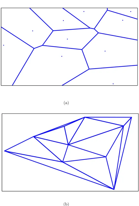
types: (a) - (b) are examples of normal tissue, (c) - (d) are ex-amples of low grade cancerous tissue, and (e) - (f) are exex-amples of high grade cancerous tissue. . . 10 2.3 An example of (a) a Voronoi Diagram and (b) a Delaunay
Trian-gulation generated for ten random points. . . 18
3.1 A schematic overview of the perturbed sample generation. . . 24 3.2 A quantized image and a sample sequence. . . 28
3.3 Sequences generated for the tissue images given in Figures 1.2(c) and 1.2(d). Similar sequences could be obtained for these two images even though they show variances at the pixel level due to their irrelevant regions. . . 29 3.4 A schematic overview of the proposed resampling-based Markovian
model (RMM) for learning the model parameters. . . 32 3.5 A schematic overview of the proposed resampling-based Markovian
model (RMM) for classifying a given image. . . 34
4.1 Performance of the algorithms as a function of the training set size: (a) the test set accuracies of the algorithms that use features similar to those of the RMM and (b) the test set accuracies of the algorithms that use features different than those of the RMM. . . 46 4.2 Performance decrease of the algorithms as a function of the training
set size: (a) the test set accuracies of the algorithms that use features similar to those of the RMM and (b) the test set accuracies of the algorithms that use features different than those of the RMM. 47 4.3 Three ROC curves of RMM which are for normal, low level
can-cerous and high level cancan-cerous classes. . . 50 4.4 The test accuracies as a function of the model parameters: (a)
window size, (b) number of states . . . 53 4.5 The test accuracies as a function of the model parameters: (a)
sequence length, (b) number of sequences. . . 54 4.6 Different types of ordering algorithms for 100 random points: (a)
greedy heuristic, (b) greedy random start, (c) Z-order, and (d) Fiedler order . . . 58
List of Tables
2.1 The Definitions of the most commonly used intensity features ex-tracted on an intensity histogram. . . 13 2.2 The definitions of the most commonly used textural features
ex-tracted on a normalized co-occurrence matrix P . . . 13 2.3 The definitions of gray level run length features on matrix Pij|θ . . 14
4.1 The parameters of the algorithms together with their values con-sidered in cross validation. . . 41 4.2 Classification accuracies on the test set and their standard
devi-ations. The results are obtained when all training data are used (when P = 100 percent). . . 43 4.3 Classification accuracies on the test set and their standard
devi-ations. The results are obtained when limited training data are used (when P = 10 percent). . . 44 4.4 Classification accuracies on the test set and their standard
devi-ations. The results are obtained when limited training data are used (P = 5 percent). . . 45 4.5 Classification accuracies obtained by the RMM that uses random
points and the RMM that uses SIFT points. . . 55
4.6 Classification accuracies obtained by RMM, RMM with intensity and RMM with cooccurrence . . . 56 4.7 Classification accuracies obtained by the RMM with a greedy
heuristic with top-left start point, the RMM with a greedy heuris-tic with random start point, the RMM with Z ordering and the RMM with Fiedler Ordering . . . 57 4.8 Classification accuracies obtained by zero-order, first-order and
Chapter 1
Introduction
Cancer is one of the most common yet most curable cancer types in western countries. Its survival rates increase with early diagnosis and selection of a cor-rect treatment plan, for which corcor-rect grading is critical [35]. Although there are many screening techniques such as colonoscopy, sigmoidoscopy, and stool test, its final diagnosis and grading are based on histopathological assessment of biopsy tissue samples. In this assessment, pathologists decide the presence of cancer based on the existence of abnormal formations in a tissue and determine cancer grade based on the degree of the abnormalities. As this assessment mainly relies on visual interpretation, it may contain subjectivity, which leads to interandintra observer variability especially in grading [3, 43]. This variability may result in suboptimal treatment of the disease [13]. Thus, it has been proposed to use com-putational methods. These methods would help pathologists make more objective assessment by providing quantitative measures.
1.1
Motivation
The previous methods provide automated classification systems that use a set of features to model the difference between the normal tissue appearance and
the corresponding abnormalities. These features are usually defined by the mo-tivation of mimicking a pathologist, who uses morphological changes in cells and organizational changes in the distribution of tissue components to detect abnor-malities. Morphological methods aim to model the first kind of these changes by extracting features that quantify the size and shape characteristics of cells. These features can be used to characterize an individual cell [57, 65] as well as an entire tissue by aggregating the features of its cells [60, 10]. Extraction of morphological features requires determining the exact locations of cells before-hand, which is, however, very challenging for histopathological tissue images due to their complex nature [28].
Structural methods are designed to characterize topological changes in tissue components by representing the tissue as a graph and extracting features from this graph. In literature, almost all methods construct their graphs considering nuclear components as nodes and generating edges between these nodes to encode spatial information of the nuclear components. These studies use different graph generation methods including Delaunay triangulations (and their dual Voronoi di-agrams) [5, 68, 58], minimum spanning trees [10, 17], probabilistic graphs [14, 30], and weighted graphs [15]. To model topological tissue changes better, Dogan et al. have recently proposed to consider different tissue components as nodes and construct a color graph on these nodes, in which edges are colored according to the tissue type of their end points [2]. The main challenge of defining struc-tural features is the difficulty of locating the tissue components. The incorrect localization may affect the success of the structural methods.
Textural methods avoid difficulties relating to correct localization of cells (and other components) defining their textures on pixels, without directly using the tis-sue components. They assume that abnormalities from the normal tistis-sue appear-ance can be modeled by texture changes observed in tissues. There are many ways to define textures for tissues; they include using intensity/color histograms [59], co-occurrence matrices [21, 18], run-length matrices [67], multiwavelet coeffi-cients [56], local binary patterns [54, 51], and fractal geometry [59, 32]. Tex-tural methods generally make pixel level analysis, hence, they may negatively be affected by the noise in the intensity levels of the pixels. Moreover, textural
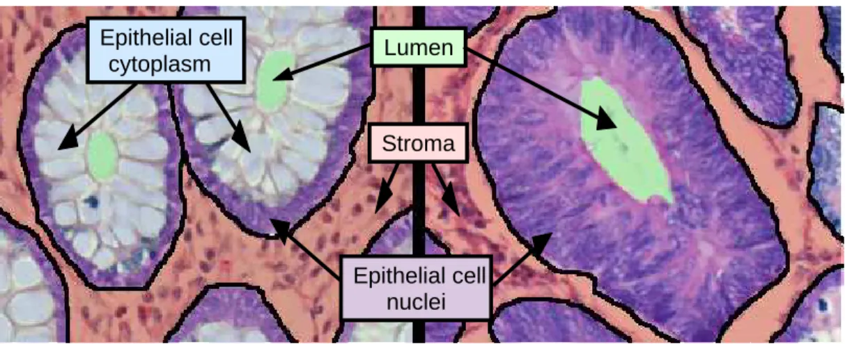
CHAPTER 1. INTRODUCTION 3 Lumen Stroma Epithelial cell nuclei Epithelial cell cytoplasm
Figure 1.1: Cytological components in normal and cancerous colon tissues. Dif-ferent components are illustrated with difDif-ferent colors: green for luminal regions, red for stromal regions, purple for epithelial cell nuclei, and blue for epithelial cell cytoplasms. Colon glands are confined with black boundaries.
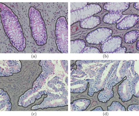
features typically characterize small regions in tissue images well but they may have difficulties to find a constant texture characterizing the entire tissue. To alleviate this difficulty, it is proposed to divide the image into grids, compute textural features on the grids, and aggregate the features for characterizing the tissue [21]. Although, grid-based approaches usually improve accuracies, they may still have difficulties arising from the existence of irrelevant regions in tis-sues. For example, for diagnosis and grading of colon adenocarcinoma, which accounts for 90-95 percent of all colorectal cancers, pathologists examine glandu-lar tissue regions since this cancer type originates from glanduglandu-lar epithelial cells and causes deformations in glands (Figure. 1.1). Non-glandular regions, which do not include epithelial cells, are irrelevant within the context of colon adenocar-cinoma diagnosis. Moreover, such non-glandular regions can be of different sizes (Figure 1.2). Thus, directly including these regions into texture computation may give unstable classifications, resulting in lower accuracies [26]. Aggregation methods that consider the existence of such irrelevant regions have potential to give better accuracies.
Additionally, all classification algorithms face a common difficulty regardless of their feature types: limited training data to be generalized to unseen cases. This problem exists in various domains such as classification of data streams [42],
(a) (b)
(c) (d)
Figure 1.2: Histopathological images of colon tissues: (a)-(b) normal and (c)-(d) cancerous. Non-glandular regions in images are shaded with gray.
remote sensing [33, 27], speech recognition [38], information theory [71], and biomedical engineering [46, 9, 62, 4]. In our domain, due to the nature of the system, there exists large variance even among tissues, even the tissues of the same class. This is mainly due to irregularity of tumor growth [32]. The variance becomes even larger due to nonideal steps followed in tissue preparation as well as differences in tissue preparation and image acquisition steps. This problem has been stated in [62] as need of large datasets for robust applications in computer aided diagnosis systems. Thus, in order for a classification system to make suc-cessful generalizations, it usually needs a large number of images from different patients in its training. On the other hand, this number is usually very limited since acquiring a large number of labeled tissue images from a large number of patients is quite difficult in this domain. When such limited data are used for training, the learned systems may be vulnerable to perturbations in tissue im-ages, also leading to unstable classifications. There have been studies in active learning to address the issue of labeling cost; the studies have proposed to reduce the number of the required samples that are to be labeled [70, 40]. However,
CHAPTER 1. INTRODUCTION 5
active learning is a selection approach of the samples to be labeled in a large dataset and does not help learn when there are only limited data available. Sim-ple resampling techniques have been used to resolve unbalanced data problem by increasing the number of samples in classes that include relatively less number of samples [49]. However, simple resampling techniques do not increase the variety since it dublicates the samples in the original dataset without introducing any modifications.
1.2
Contribution
In this thesis, we propose a new framework for the effective and robust classi-fication of tissue images even when only limited data are available. In the pro-posed framework, the main contributions are the introduction of a new resampling method to simulate the perturbations in tissue images for learning better gen-eralizations and the use of this method for obtaining more stable classifications. The resampling method relies on generating multiple sequences from an image, each of which corresponds to a perturbed sample of the image, and modeling the sequences using a first order discrete Markov process. Working with colon tissue images, our experiments show that such a resampling method is effective in increasing the generalization capacity of a learner by increasing the size and variation of the training set as well as boosting the classifier performance for an unseen image by combining the decisions of the learner on multiple sequences of that image.
This study differs from the previous tissue classification methods in two main aspects. First, it proposes a new framework in an attempt to alleviate an issue of having limited labeled training data. For that, it introduces the idea of generating “perturbed images” from the training data and modeling them by a Markov process. Although the issue of having limited training data is acknowledged by many researchers working in this domain, it has rarely been considered in the design of tissue classification systems. Second, it proposes to classify a new image using its perturbed samples. The use of different perturbations of the same image
is more effective to reduce the negative outcomes of large variance observed in tissue images, as opposed to the use of the entire images at once. Moreover, modeling the perturbations with Markov processes provides an effective method in modeling the irrelevant regions.
1.3
Outline of the Thesis
This thesis is structured as follows. In Chapter 2, we give background information about the problem domain and summarize the existing approaches from litera-ture. In Chapter 3, we present the details of our method including how perturbed samples from an image are generated and how these perturbed samples are used in learning and classification by modeling them with Markov chains. In Chapter 4, we explain the dataset, the test environment, and comparison methods. Then, in the same chapter, we report the test results and give a discussion of the results. Finally, we finalize the thesis with a conclusion and its future aspects, in Chapter 5.
Chapter 2
Background
In this chapter, we first present domain description in which we explain a specific cancer type colon adenocarcinoma and how colon tissues undergo deformation as a consequence of adenocarcinoma. Then we explain the classes that a tissue image can be classified to and how they are different from each other. Next, we present a summary of textural, morphological, and structural approaches in the literature for automated cancer diagnosis. Finally, we discuss the problem of having limited training dataset and discuss active learning, semi-supervised learning and resampling techniques.
2.1
Domain Description
In this thesis, we focus on colon adenocarcinoma, which is estimated to be respon-sible of 90-95 percent of all types of colorectal cancer. Colorectal cancer is the third most common cancer type among men and women in the USA [35]. Colon adenocarcinoma affects glandular tissue in the inner wall of the colon, which is re-sponsible for secreting materials to lubricate waste products and absorbing water and some minerals from waste products before excretory. Colon adenocarcinoma starts at inner wall of the colon then spreads to the entire colon, potentially to the lymphatic system and the other organs as well. If it spreads, it may be fatal.
However, colon adenocarcinoma is one of the most curable cancer types if it is early detected. Screening tests such as colonoscopy and flexible sigmoidoscopy help early detection of colon adenocarcinoma without need of the surgery and ac-cording to [35] there is an observed decrease of colon adenocarcinoma due to the increased prevalence of these tests. Although these screening tests are important at early detection of colon adenocarcinoma. The final diagnosis together with its grade, can be made after examining biopsy sample by a pathologist under a mi-croscope. For that, a small amount of the tissue of the concerned area is removed from the human body, and then this removed tissue is cut into thin slices. These thin slices are named as sections and the process is known as sectioning. Sub-sequently, for better visualization of these sections under a microscope, they are stained with a chemical process, which is named as staining. Staining gives con-trast to the tissue, highlighting its special components for better visualization. The routinely used staining technique is hematoxylin and eosin. Hematoxylin stains nucleic acids deep blue and eosin stains cytoplasm pink as a result of a chemical reaction [24]. An illustrative example of an histopathological image from a colon tissue is given in Figure 2.1.
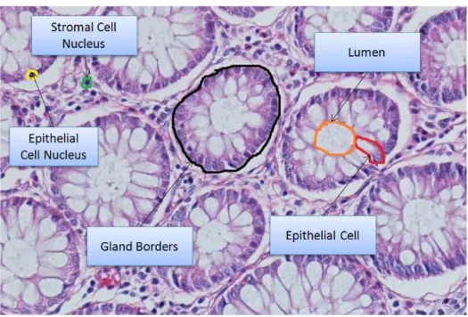
In Figure 2.1, cytological components of a colon tissue are also illustrated. The most important components for colon adenocarcinoma are glands. Glands involve relatively large luminal areas and epithelial cells surrounding these lu-mens. Lumens are white large regions in Figure 2.1 and they are responsible for absorption of water and minerals and secretion of mucus to waste products. Epithelial cell nuclei are stained dark purple and forms the border of the glands. Stroma is the region that connects glands and keeps them together. In stroma, there exist non-epithelial cells, which are also stained dark blue. Colon adeno-carcinoma originates from epithelial cells and changes glands’ structure, shape, and size. From a low grade gland to a high grade gland, the change becomes considerable. In this thesis, we focus on three classes (tissue types) in the con-text of diagnosis of colon adenocarcinoma. These tissue types are normal, low grade cancerous and high grade cancerous. These tissue types are exampled in Figure 2.2. As seen in Figure 2.2(a)-(b), a normal tissue does not include any cancer or there is no deformation on the structure of glands. With the beginning
CHAPTER 2. BACKGROUND 9
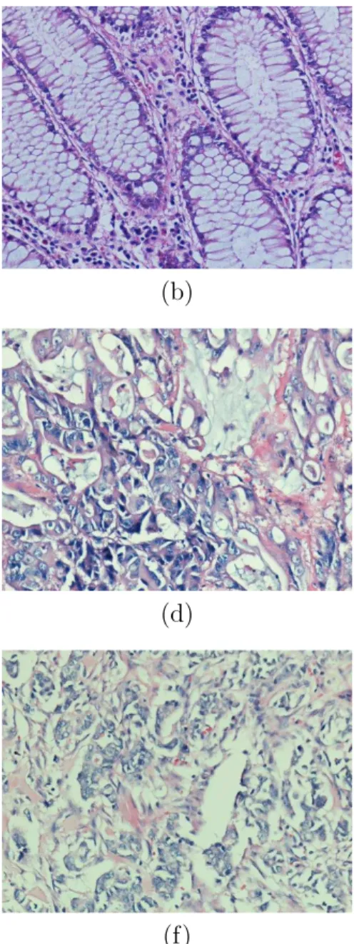
Figure 2.1: An example of a colon tissue stained with hematoxylin-and-eosin. of the cancer, glands undergo changes in their structure; however, glands are still well to moderately differentiated in tissue images as seen Figure 2.2(c)-(d). When the cancer advances, a tissue turns into a high grade cancerous tissue. In a high grade cancerous tissue, since the deformation on the glands are too much, gland structures are only poorly differentiated, as seen in Figure 2.2(e)-(f)
(a) (b)
(c) (d)
(e) (f)
Figure 2.2: An illustration of example tissue images from different cancer types: (a) - (b) are examples of normal tissue, (c) - (d) are examples of low grade cancerous tissue, and (e) - (f) are examples of high grade cancerous tissue.
CHAPTER 2. BACKGROUND 11
2.2
Automatic Cancer Diagnosis
In this section, we briefly summarize the existing computational methods pro-posed for automated cancer diagnosis. We group these methods into three main categories: morphological, textural, and structural.
2.2.1
Morphological Methods
Cancer causes deformation in the shapes of cells and nuclei components in a tis-sue. Morphological methods attempt to recognize cancer in the tissue by modeling these changes with numerical features that characterize the shape and size of these components. These features can also be aggregated to model the entire tissue by computing their average and standard deviation [60, 10]. In literature, there are various morphological features defined for quantifying cells/nuclei. Commonly used features include radius, perimeter, area, compactness, smoothness, concav-ity, symmetry, circularconcav-ity, and eccentricity [57, 50]. Nucleocytoplasmic ratio, hy-perchromasia, aninonucleosis, and nuclear deformity measures are other features for cell/nucleus quantification [60]. There are also some studies that combine the morphological features with other types of features to obtain a larger set of features. For example, in [65], the morphological features are used along with textural features for characterizing a tissue.
Extraction of morphological features requires determining the exact locations of cells beforehand, which is, however, very challenging for histopathological tissue images due to their complex nature [28]. This problem becomes a bottleneck for the morphological methods and inexact localization of the nuclei components may affect the success of these methods in negative manner.
2.2.2
Textural Methods
The existence of cancer changes texture and color of a tissue. Textural meth-ods aim to capture these changes by extracting textural features from the tissue
image. One advantage of using textural features over using morphological and structural features is that it does not require segmentation of tissue components beforehand. There are various texture extraction methods employed for charac-terizing a tissue. For example, intensity and color histograms are used to model the color changes; Haralick features extracted from co-occurrence matrices utilize second order statistics of gray level intensity distribution; fractal geometry fea-tures allow quantitative representation of complex and irregular shapes; wavelet features contain information of an image at different scales. In the next subsec-tions, we briefly mention these textural features.
2.2.2.1 Intensity and Color Histogram Features
In hematoxylin-and-eosin staining, there exist color changes when a tissue is can-cerous. This can be attributed to the spread of nuclei, which are stained blue or purple, to stroma and lumina. Since, nuclei cover larger areas in cancerous tis-sues compared to normal ones, such tistis-sues include large areas with low intensity values. Color histograms are used to model these changes [59]. To this end, the intensity value of each pixel in red, green, and blue channels can be discretized into N bins and the frequency of each bin is stored in a histogram.
Likewise, intensity features model the distribution of gray level intensities of pixels in tissue images. These features are extracted from gray level inten-sity histograms and they include mean, standard deviation, skewness, kurtosis, and entropy of the gray level distribution [69]. In order to extract these fea-tures, the histogram probability density function h(gi) is first computed such that P
ih(gi) = 1. The intensity features are then computed on this density function. The definitions of the most commonly used intensity features are given in Table 2.1.
CHAPTER 2. BACKGROUND 13
Table 2.1: The Definitions of the most commonly used intensity features extracted on an intensity histogram. Mean m =P i h(gi) · gi Standard deviation σ =P i (gi− m)2· h(gi) Skewness s =P i (gi− m)3· h(gi) Kurtosis k ==P i (gi− m)4· h(gi) Entropy e = −P i h(gi) · log2h(gi)
2.2.2.2 Co-occurrence Matrix Features
Co-occurrence matrix features are defined to characterize the spatial distribution of gray level intensity values in an image [31]. The co-occurrence matrix P is defined as a matrix that keeps the frequency of two gray levels being co-occurred in a particular spatial relationship defined by a distance d and an angle θ. Second order statistics are computed on the matrix P to obtain co-occurrence matrix features. The most commonly used co-occurrence features are listed in Table 2.2. In the table, Pij stands for frequency of gray levels i and j being co-occurred, µx and µy are the means of column, row sums, and σx and σy are their standard deviations. In histopathology tissue domain, co-occurrence features are often used to characterize the texture of an entire tissue image [69, 19, 18, 36].
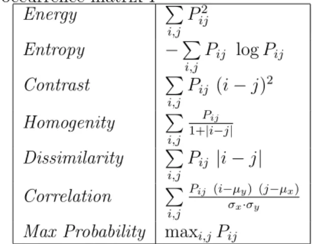
Table 2.2: The definitions of the most commonly used textural features extracted on a normalized co-occurrence matrix P
Energy P i,j Pij2 Entropy −P i,j Pij log Pij Contrast P i,j Pij (i − j)2 Homogenity P i,j Pij 1+|i−j| Dissimilarity P i,j Pij |i − j| Correlation P i,j Pij (i−µy) (j−µx) σx·σy
2.2.2.3 Gray Level Run Length Features
In statistical texture analysis, the number of combination of intensity levels de-termines the order of the statistics used for feature extraction. Features extracted from intensity and color histograms are examples of the first-order statistics, while co-occurrence features are examples of the second-order statistics. Gray level run length features are examples of higher order statistical texture features [1]. A gray level run is a set of consecutive pixels with the same gray level intensity in a given direction. The run length is defined as the number of pixels in a run and the run length value is the frequency of this run in an overall image. A gray level run length matrix P includes Pij|θ that gives the total number of runs of a length j and a gray level intensity i at direction θ. Galloway introduces five features to be extracted from a gray level run length matrix [25] and Chu later extends them by defining two new features [11]. These features are summarized in Table 2.3, where n is the total number of pixels in the image. Let K be the total number of runs in the image such as K =P
i P
j Pij|θ.
Table 2.3: The definitions of gray level run length features on matrix Pij|θ
Short Runs Emphasis P
i P
j Pij|θ
j2 / K
Long Run Emphasis P
i P
j
j2 Pij|θ / K
Gray Level Non-uniformity P
i (P
j
Pij|θ)2 / K
Run Length Non-uniformity P
j (P
i
Pij|θ)2 / K
Run Percentage n1K
Low Gray Level Runs Emphasis P i
P
j Pij|θ
i2 / K
High Gray Level Runs Emphasis P i
P
j i2 P
ij|θ / K
In the diagnosis of cancer, gray level run length features are generally used together with other features. For instance, Bibbo et al. use gray level run length features along with co-occurrence and intensity features to distinguish normal and tumor nuclei. [6]. Weyn et al. use gray level run length features and co-occurrence features to statistically characterize nuclei of an image [66].
CHAPTER 2. BACKGROUND 15
2.2.2.4 Fractal Geometry Features
Fractal geometry features are used at characterizing complex and irregular shaped objects in images [37]. A fractal is an object made of subobjects that are similar to the whole object in some way. Fractal dimension D gives the complexity of a fractal. Self similarity can be used to estimate the fractal dimension D. For example, let S be a self similar object which is union of Nr distinct copies of S scaled down by ratio r. We can estimate fractal dimension D of S by the expression Nr· rD = 1 or D can be calculated by the following equation.
D = −log Nr log r
However, most of the natural objects do not show deterministic self similarity so fractal dimension D should be estimated. There exist different methods to estimate fractal dimension, one of the most commonly used technique is differ-ential box-counting approach. Most of the time together with other types of features, fractal features are used to characterize texture of the histopathological images [32, 59].
2.2.2.5 Multiwavelet Features
In wavelet transform, the data is first divided into different frequency components and they are analyzed at resolution matching to their scale [29]. Multiwavelet transform uses more than one scaling function. Multiwavelet transform can pre-serve features such as short support, orthogonality, symmetry, and vanishing mo-ments [56]. Zadeh et al. use multiwavelet features in histopathology images for automated Gleason grading of prostate tissues. To do so, using wavelet transform, they compose each tissue image into subbands. Finally, from wavelet coefficients of the subbands, they extract features such as entropy and energy to characterize the tissue image [56]. It is also possible to select distinctive subbands and use them for feature extraction [51].
2.2.2.6 Local Binary Pattern Features
Local binary patterns are a set of textural features that are used to model the texture of an image in micro-level. In this technique, a binary number is generated for each pixel in the image and these numbers are combined using a histogram. This histogram is used as a feature vector to characterize the texture of the image. To generate a binary number for a pixel, a 3 × 3 operator is used to compare its intensity with its neighbors’ intensities; it assigns zero if a neighbor’s intensity is lower than the pixel’s intensity, otherwise it assigns one. These binary values for each neighbor are appended in clock-wise manner to obtain a binary number for the pixel [48]. Qureshi et al. extend local binary patterns by choosing neighbors of a particular pixel from those that lie on a circle which is centered on that particular pixel and has a radius of r [51]. Sertel et al. use local binary pattern features and co-occurrence matrix features together for detection of cancer in histopathological images [54].
2.2.3
Structural Approaches
Structural approaches aim to recognize cancer from the topological changes of tissue components in cancerous tissues. Structural methods usually represent the tissue with a graph to model spatial distribution and neighborhood informa-tion of tissue components. Features extracted from these graphs are used in the automated cancer diagnosis and grading. In generation of such graphs, nuclear components are usually considered as graph nodes and edges are generated to re-tain spatial information among these nodes. There are various graph generation methods; these graphs include Delaunay triangulations, Voronoi diagrams, mini-mum spanning trees, probabilistic graphs, and weighted graphs. Recently, color graphs are used for tissue characterization. In addition to nuclear components, this approach also considers other cytological components in its graph generation. In the next subsection, we briefly mention some of these methods.
CHAPTER 2. BACKGROUND 17
2.2.3.1 Voronoi Diagram Features
A Voronoi diagram is the partitioning of a plane into complex polygons C = {Ci}Ni=1 with given points O = {oi}Ni=1 such that there exists exactly one gener-ating point oi for the complex polygon ci and each point residing in the polygon ci is closer to its generating point oi than other generating points O \ {oi} [68]. Figure 2.3(a) shows an example of a Voronoi diagram generated on ten random points. Voronoi diagrams are also commonly used in the structural representation of histopathological images [5, 68, 58, 19]. To this end, the set of nuclear cen-troids on a tissue image is used as generating point set O and a Voronoi diagram is constructed on this point set. Commonly extracted features from a Voronoi diagram include the mean, standard deviation, min-max ratio, and disorder of polygon areas, the polygon perimeter lengths, and the polygon chord lengths [5].
2.2.3.2 Delaunay Triangulation Features
The Delaunay triangulation can be derived from a Voronoi diagram as they are dual of each other. The Delaunay triangulation D of a given point set O = {oi}Ni=1 can be constructed easily after its Voronoi diagram V is generated. For that, an edge is assigned between any two unique points, oi and oj, where i 6= j, if their corresponding polygons, ci and cj, in the V share a side. Figure 2.3(b) illustrates the Delaunay triangulation generated on ten random points. In histopathologi-cal image domain, many studies use Voronoi diagrams together with Delaunay triangulation to characterize the structural information of a tissue image [5, 19]. Likewise, these studies use nuclear centroids to generate Delaunay triangulation. Common features extracted from the Delaunay triangulation consist of the mean, standard deviation, min/max ratio, and disorder of the triangle edge lengths and the triangle areas.
(a)
(b)
Figure 2.3: An example of (a) a Voronoi Diagram and (b) a Delaunay Triangu-lation generated for ten random points.
CHAPTER 2. BACKGROUND 19
2.2.3.3 Minimum Spanning Tree Features
A spanning tree of a connected and undirected graph G is a subgraph that con-nects all of the graph nodes without having any cycles. There may exist differ-ent spanning trees of the same graph. For the weighted graphs, the minimum spanning tree (MST) is defined as the one that minimizes the total spanning tree edge weights. In automatic cancer diagnosis, features extracted from min-imum spanning trees are used to characterize a tissue. These features include the mean, standard deviation, min/max ratio, and disorder of the MST edge lengths [10, 17, 19, 68, 5].
2.2.3.4 Color Graphs Features
As opposed to other structural methods, which model only the spatial distribution of cell nuclei using a graph, the color graph approach is proposed to model also the distribution of other tissue components [2]. In this approach, a graph is generated considering nuclear, stromal, and luminal tissue components as graph nodes and assigning graph edges using Delaunay triangulation. In this graph representation, each edge is labeled according to the type of their end nodes. After constructing a graph, colored version of the features such as the colored average degree, colored average clustering coefficient, and colored diameter are extracted.
2.3
Limited Training Data
In supervised classification, a model is first learned from a training set and then used to classify unlabeled samples. Here the aim is to construct a good model, which is a close approximation to the true model. The difference between the con-structed and true models may yield an error, which is also known as an estimation error. In order to construct a good model, and hence to reduce the estimation er-ror, it is known that the model should be learned on sufficient, and usually large, amount of labeled training samples, which reflect the real data distribution [20].
On the other hand, obtaining large amount of labeled data is quite difficult, and costly, in many problem domains. Automated cancer diagnosis on histopathologi-cal images is one of such domains. To alleviate this problem, different approaches have been proposed. Active learning, which intelligently selects the samples to be labeled, is one them [40, 70] it is also possible to use semi-supervised learning, which combines labeled and unlabeled data in the construction of a classifier [39]. Another approach is to use data resampling, which is especially used to make unbalanced dataset balanced [12, 49].
2.3.1
Active Learning
Active learning methods assume that collecting unlabeled data is easy but labeling them is costly and difficult [55]. Therefore, in active learning systems, a classifier selects the samples to be labeled (and to be used in its training set) interactively. Here the aim is to obtain the highest accuracies by selecting the minimum number of samples. For that, it is possible to start with random selection of samples as an initial training set and enhance the classifier iteratively by selecting and labeling unlabeled samples. To select an unlabeled sample, Liu et al. calculate the distance of unlabeled samples to the SVM’s hyperplane and select the sample with the highest distance. They apply this approach to gene expression data for cancer classification [40]. Yu et al. use a classifier to estimate the confidence score of an unlabeled sample, and decide whether or not to label the sample according to its score level. The classifier labels the sample if its confidence level is higher than a predefined threshold, the classifier leaves the sample to be labeled by an expert otherwise [70].
2.3.2
Semi-supervised Learning
Similar to active learning, semi-supervised learning assumes that a large number of unlabeled data exists in the dataset, however labeling them is difficult. This approach utilizes unlabeled samples to increase the performance of the classifier
CHAPTER 2. BACKGROUND 21
especially where there is a limited number of labeled training samples. As op-posed to active learning, semi-supervised learning does not query the label of the unlabeled samples to an expert, this is the difference between semi-supervised learning and active learning. In [39], they use ensemble of N classifiers. To refine a particular classifier, they use other classifiers to label an unlabeled sample, and they use the labeled sample in the particular classifier’s training set.
2.3.3
Resampling
In resampling, samples are drawn from a sample set to obtain a new set [45]. Resampling has been used with different purposes including validation of cluster results [45] and performance evaluation of classifiers [63, 53]. Additionally, it is commonly used to alleviate negative effects of the issue of unbalanced training datasets problems [47, 22, 12, 49]. In unbalanced datasets which the number of samples is significantly different from each other among classes, classifiers tend to favor prevalent classes. To circumvent this problem, one may balance the dataset by resampling from classes with less number of samples. There are three techniques:
• Bootstrapping: In bootstrapping, each bootstrap sample is obtained by random selection from the original dataset with replacement. In this re-sampling technique, some samples in the original set may be selected more than once or may not be selected at all. In subsampling, random subsets {Yi}Ni=1 are resampled from the set X such that Yi ⊂ X [45].
• Jittering : If one measures the same event multiple times, these measure-ments may be different from each other due to the measurement error. In jittering, the main motivation is to simulate the existence of such measure-ment errors in selecting samples. Hence, jittering selects random samples from the original dataset and adds random noise to these selected sam-ples [45].
• Perturbation: In bootstrapping, resampled samples are the replicates of the original samples. Likewise, in jittering, resampled samples are only
slightly different from the original ones. These resampling techniques do not simulate the differences between samples due to the intra-population variability. On the other hand, perturbation attempts to reflect estimates of intra-population variability to the original samples. In this technique, random variables are generated from a distribution that models distribu-tion of original samples and these random variables are added to original samples to obtain perturbed samples [45]. For example, one may calculate the mean and standard deviation of the original samples, calculate random values from a normal distribution with the computed mean and standard deviation, and add these values to original samples [45].
Although these techniques increase the size of a dataset, however, for images that contain irrelevant information and a considerable amount of noise, one may want to develop techniques that do not use the entire image but some of its sub-regions. In this thesis, we present a novel resampling technique. This technique generates sequences that model partial regions in the tissue image and uses each of these sequences as a sample in learning and classification.
Chapter 3
Methodology
The proposed resampling-based Markovian model (RMM) relies on generating perturbed samples from each tissue image and using these perturbed samples in learning and classification. The main motivation behind the use of perturbed samples is to model variances in tissue images better even when only limited labeled data are available. The RMM includes two components: perturbed sam-ple generation and Markov modeling. We explain these two components in the following sections.
3.1
Perturbed Sample Generation
Let I be a tissue image that is to be either classified in testing or used in training. The RMM represents this image by N of its perturbed samples, I = {S(n)}N
n=1, each of which is represented by a sequence of T observation symbols, S(n) = O1(n)O2(n). . . OT(n). (For better readability, we will drop n from the terms unless its use is necessary. Thus, each perturbed sample is represented by S = O1O2. . . OT.) These perturbed samples model partial regions of the tissue image I. There are three main steps: The first step is the selection of data points and extracting features representing them, the second step is to discretize extracted features into a set of observation symbols, and the final step is to order the observation
symbols. These steps are explained in Sections 3.1.1, 3.1.2, and 3.1.3, respectively. Figure 3.1 illustrates the general outline of the perturbed sample generation.
Figure 3.1: A schematic overview of the perturbed sample generation.
3.1.1
Random Point Selection and Feature Extraction
The first step of generating a sequence S from the image I is to select T data points from the image I and to characterize them by extracting features. The RMM uses random point selection to select T random points. After selection of T data points, each point is characterized by using its neighborhood pixels. To this end, we locate a window centered on each of these selected points and extract features to characterize the local image around this point. The RMM uses four features that quantify color distribution and texture of the pixels falling within this window. These four features are defined on the quantized pixels. The quantization of the pixels is mapping pixel colors to some dominant colors. In our case, tissues are stained with hematoxylin and eosin, which yields three dominant colors (white, pink and purple). However, the intensity levels of these three dominant colors show differences among tissue images due to the variability of the staining process. In quantization of pixels we map pixel colors into white, pink and purple. For that reason, the k-means algorithm is used to cluster pixel colors of the image I into three and each of these clusters are labeled as white,
CHAPTER 3. METHODOLOGY 25
pink or purple according to closeness of the center of the cluster to these three dominant colors. The first three features that the RMM uses correspond to ratios of quantized pixel colors in the window. The last feature is a texture descriptor (J -value) that quantifies how uniform the quantized pixels are distributed in space [16]. Let Z be the set of the pixels that reside in the window and Zi be the set of the pixels that belongs to color i; in our case, since we quantize pixel colors, i might be either white, pink or purple. Let z = (x, y) ∈ Z be a pixel. We first calculate the overall mean m of the pixels in Z, and class mean mi for the pixels in Zi. m = P z∈Z z |Z| (3.1) mi = P z∈Zi z |Zi| (3.2) Then, we calculate overall variation Stand total variation of pixels belonging the same class Sw. St = X z∈Z ||z − m|| (3.3) Sw = X i∈{white,pink,purple} X z∈Zi ||z − mi|| (3.4)
The J -value is calculated from St and Sw.
J = Sw− St St
(3.5) Note that, the RMM uses a generic feature framework and does not impose any specific feature type. One may define his/her own features and use them in the RMM. In this study, we select features that are effective and easy to compute. Besides, selected features do not introduce any external model parameters.
In this step, for the selection of data points, we use random selection by default, yet there would be other methods for the selection of these T data points. For example, one may want to identify SIFT (Scale Invariant Feature Transform) points from the image I, which are commonly used in object detection in the literature [41]. We discuss the effects of selecting of the data points randomly or via SIFT in Section 4.5.2.1.
3.1.2
Discretizing Features into Observation Symbols
After selecting data points and extracting their features, we discretize the features for the data points into K observation symbols, {vk}Kk=1, since we use discrete Markov processes for modeling different types of tissue formations. There are two main steps for the discretization. The first step is the unsupervised learning of the observation symbols; this step is done once and learned observation symbols are used throughout the learning and classification stages. The second step is to discretize each of the features to an observation symbol. The details of these steps are explained in the following subsections.
3.1.2.1 Learning Observation Symbols
We use k-means clustering to learn K clusters on the extracted features of the data points selected from the training images. K-means is an unsupervised clus-tering that partitions the data points such that the squared error between the mean of a cluster and the points in that cluster is minimized [34]. It is an it-erative algorithm that minimizes the squared error in each iteration. We learn clusters by selecting 100 random data points from each training image and initial-ize k-means with random initial cluster centers. Although the number of selected points does not have too much effect for larger training sets, its smaller values lead to decreased performance when smaller training sets are used. In general, this number should be selected large enough so that different “good” clusters can be learned. However, it may be selected smaller to decrease the computational time of training. In addition, note that unsupervised learning of the observation symbols provides the RMM the flexibility of automatic observation symbol learn-ing. Hence, the RMM can easily be extended to other domains or to other feature types. One can change the feature extraction process and apply the RMM in the areas outside of histopathological image classification.
CHAPTER 3. METHODOLOGY 27
3.1.2.2 Discretizing Features
After we find {vk}Kk=1observation symbols, we map extracted features of a selected point to one of the {vk}Kk=1 observation symbols. Let {mk}Kk=1 be the set of the cluster centers that each observation symbol corresponds. For each selected point P , we have a set of four features which can be denoted by X. We discretize P to the observation symbol v∗ that is the label of the closest cluster center.
v∗ = argmin i
dist(X, mi) (3.6)
Here, we use the Euclidean distance to compute the distance between the X and each cluster center. At the end of this step, a perturbed sample is represented with a set of observation symbols, S = {Oi | Oi = vk where 1 ≤ k ≤ K for all i}, but not as a sequence of them.
3.1.3
Ordering the Points
The next step is to order the data points and construct a sequence from their observation symbols. The data points are ordered as to minimize the sum of distance between the adjacent points. Formally, this ordering problem can be represented as finding S = O1O2. . . OT such that
T X
t=2
dist(Pt−1, Pt) (3.7)
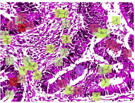
is minimized. Here dist(u, v) represents the Euclidean distance between the points u and v and Otis the observation symbol defined for the point Pt. This formulated problem indeed corresponds to finding the shortest Hamiltonian path among the given points, which is known as NP-complete. Thus, the proposed method uses a greedy solution for ordering. This greedy solution selects the point closest to the top-left corner as the first data point P1 and then at every iteration t, it selects the data point Pt that minimizes dist(Pt−1, Pt). In Figure 3.2, we illustrate a quantized image and a perturbed sample generated from this quantized image. Note that for simplicity, we select length of the sequence as 40 and number of the distinct states as 10. We repeat this process to obtain N sequences.
Figure 3.2: A quantized image and a sample sequence.
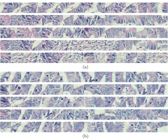
At the end of this step, we obtain N sequences, each representing a perturbed image. These sequences are expected to model variances in tissue images bet-ter. To illustrate the reason behind this, let us consider the tissue images in Figures 1.2(c) and 1.2(d). Although they show variances at the pixel level due to their irrelevant regions, these images are indeed very similar to each other in terms of their biological context. Figures 3.3(a) and 3.3(b) show some sequences generated from these images; here a data point is represented with its window, in which its features are extracted. As observed in these figures, it is possible to obtain similar sequences for these two images; the first three sequences of Fig-ure 3.3(a) are visually similar to those of FigFig-ure 3.3(b). In our proposed RMM, we anticipate to have some of such similar sequences provided that a large number of sequences are generated.
Generating perturbed samples increases number of samples in the dataset. Besides, it also increases the diversity. For instance, if we extract features using an entire image, we would obtain one feature vector representing the entire image. However with perturbed sample generation, we model different parts of the image
CHAPTER 3. METHODOLOGY 29
(a)
(b)
Figure 3.3: Sequences generated for the tissue images given in Figures 1.2(c) and 1.2(d). Similar sequences could be obtained for these two images even though they show variances at the pixel level due to their irrelevant regions.
and use the information from these different parts for learning and classification. Moreover, although each of these sequences is generated from the same image, they are different from each other. For instance in Figure 3.3(a) or 3.3(b), the perturbed samples are generated from the same image and they are directly related to the same image, however as you observe, they are different from each other and some of these sequences even do not resemble to each other. Hence, by using perturbed samples, we increase the diversity in the training set.
3.2
Markov Modeling
A Markov process models the state of a system with a random variable X which changes with time. For instance, X1 gives the state of the system at time one. A
Markov model is a stochastic process, where the value of the Xt depends on its previous s states. For example, in the first-order Markov model, s becomes one; i.e., the future behavior of the system (state of system) depends on its previous state. A discrete Markov model is a Markov process whose state space is a finite set. There are two common types of Markov models: observable and hidden Markov models. In an observable Markov model, the states are equivalent to the observations; that is with the knowledge of observation, we can precisely infer the state. In a hidden Markov model, the observations are related to underlying state, but the knowledge of observation is insufficient to precisely infer the underlying state.
In the proposed RMM, we model the perturbed samples each of which is a sequence of observation symbols S = O1O2. . . OT with Markov models. In addition, we assume one-to-one correspondence with observation symbols and states, and a finite set of the observation symbols. These assumptions allow us to use a m’th order observable discrete Markov model. In this study, we use m = 1, so observation symbol Ot is only dependent to its previous observation symbol Ot−1.
P (Ot= vi | Ot−1= vj, Ot−2 = vk, . . .) =
P (Ot= vi | Ot−1= vj) (3.8)
In this study, we use Markov modeling since it is one of the simplest and most effective ways of modeling sequences. There are also other possible methods for sequence modeling such as hidden Markov models and recurrent neural networks. We believe that these methods can work well in the proposed method, provided that their parameters are correctly estimated on the training data. However, since Markov modeling provides a fairly accurate tool for our purpose and because of its simplicity, we prefer using it.
CHAPTER 3. METHODOLOGY 31
3.2.1
Learning the Parameters of a First Order
Observ-able Discrete Markov Model
For each class Cm, we train a different Markov model. Each Markov model has three parameters: the number of states (observation symbols) Km, initial state probabilities Πm = {π(vi | Cm)}, and state transition probabilities Am = {a(vi, vj | Cm)} where
π(vi | Cm) = P (O1 = vi | S ∈ Cm) (3.9) a(vi, vj | Cm) = P (Ot+1 = vj | Ot= vi and S ∈ Cm) (3.10)
The number of states Km is the same for every Markov model and equal to the number of observation symbols. For learning the probabilities Πm and Am, a new training set, Dm = {S(u) | S(u) ∈ Cm}, is formed generating N perturbed samples from each training image that belongs to the class Cm. Using this new training set, the probabilities are learned by maximum likelihood estimation. The process is illustrated in Figure 3.4.
π(vi | Cm) =
#{S(u) such thatO1(u) = vi}
#{S(u)} (3.11)
a(vi, vj | Cm) = T −1
P
t=1
#{S(u) such that O(u)
t = vi, O (u) t+1 = vj} T −1 P t=1
#{S(u) such that O(u) t = vi}
(3.12)
In Equations 3.11 and 3.12, #{.} denotes ”‘number of”’ function. In these equations, if there is no occurrence of a particular event in the training data, then the formulas yield zero probability for those events. For example, if there is no subsequent observation of vi and vj in any sequence in the training set, the state transition probability a(vi, vj) will be zero. This case may not be desired especially when there is limited data for training, since many probabilities will be zero, although the occurrence of these events would be plausible. Zero probability
is indeed very ambitious, as not having an observed occurrence of an event does not really mean it will not happen. In order to handle this problem, in this study, we use additive smoothing [8] with α = 1. Additive smoothing assumes an occurrence of each event from the outset. The α parameter gives initial frequency to each possible event. Therefore, the initial and transition probabilities can be computed as
π(vi | Cm) =
#{S(u) such that O(u)1 = vi} + α
#{S(u)} + α · K (3.13)
a(vi, vj | Cm) = T −1
P
t=1
#{S(u) such thatO(u)t = vi, O(u)t+1= vj} + α T −1
P
t=1
#{S(u) such thatO(u)
t = vi} + α · K
(3.14)
Figure 3.4: A schematic overview of the proposed resampling-based Markovian model (RMM) for learning the model parameters.
3.2.2
Classification
The classification of a given image I is done using its perturbed samples. For each perturbed sample S ∈ {Si}Ni=1 of I, the posterior probability of each class Cm is
CHAPTER 3. METHODOLOGY 33
computed and the class that maximizes these posterior probabilities is selected. Posterior probability P (Cm | Si) is the probability of the perturbed sample Si belonging to class Cm. Subsequently, the class C∗ of the image I is found using a majority voting scheme that combines the selected classes of the perturbed samples of I. δki = ( 1 if k = argmaxmP (Cm | Si) 0 otherwise (3.15) C∗ = argmax j N X i=1 δji (3.16)
The posteriors P (Cm | S) are calculated by the Bayes rule: P (Cm | S) = P (S | Cm) · P (Cm) P (S) (3.17) where P (S) =X m P (S|Cm) · P (Cm) (3.18)
In the Bayes rule, there are two unknowns, the first one is class probabili-ties P (Cm). In this study, we assume that each class is equally likely that is P (C1) = P (C2) = ... = P (Ci) = ... = P (Cm). The other unknown is the class likelihood P (S | Cm). Once Πm and Am are learned on the training sequences, class likelihood P (S | Cm) can be written as
P (S | Cm) = π(O1 | Cm) T −1 Y
t=1
a(Ot, Ot+1 | Cm). (3.19)
Since we assume the equal class prior probabilities, the class m that maximizes class likelihood P (S | Cm) will also maximize posterior probability P (Cm | S). The steps of the RMM to classify an unseen image are given in Figure 3.5.
Figure 3.5: A schematic overview of the proposed resampling-based Markovian model (RMM) for classifying a given image.
Chapter 4
Experiment Results
In this chapter, we first give the details of the dataset and explain the methods that we compare with the proposed RMM. Then we describe the cross-validation technique that is used in parameter selection of the RMM and other methods. Next, we present the results of our experiments conducted with different training data sizes to understand how accurate and stable the RMM is against other al-gorithms. Finally, we discuss the results and give the detailed parameter analysis of the RMM.
4.1
Dataset
The dataset used in the experiments contains 3236 microscopic images of colon tissues of 258 randomly selected patients from the Pathology Department archives in Hacettepe University School of Medicine. The tissues are stained with hema-toxylin and eosin and their images are taken with a Nikon Coolscope Digital Microscope using 20× microscope objective lens at 480 × 640 image resolution. This magnification level is high enough to ensure that different regions in a tissue image are in the same class in the context of cancer diagnosis. In addition, it is low enough to demonstrate many instances of glands in the same image.
We randomly divide the patients into two such that the training set contains 1644 images of the first half of the patients and the test set contains 1592 images of the remaining. We label each image with one of the three classes: normal, low-grade cancerous, or high-grade cancerous1. The training set contains 510 normal, 859 low-grade cancerous, and 275 high-grade cancerous tissues. The test set contains 491 normal, 844 low-grade cancerous, and 257 high-grade cancerous tissues. As you may notice, the dataset we use is unbalanced and may favor low-grade cancerous class. In order to obtain unbiased results, we resample normal and high-grade cancerous tissue images randomly until we have balanced number of samples for all class types.
4.2
Comparisons
To investigate the effectiveness of the proposed method, we compare its results with those of the two sets of algorithms. The first set includes algorithms that define their features similar to the RMM but take different algorithmic steps for classification. We particularly implement these algorithms to understand the effectiveness of the perturbed sample generation and Markov modeling steps proposed by the RMM. The second set includes algorithms that use different textural and structural features proposed by existing methods. We use them to compare the performance of the RMM and previous approaches. In these algorithms, we use SVM with a linear kernel for classification.
4.2.1
Algorithms with Similar Features
4.2.1.1 GridBasedApproach
First, we implement a grid-based counterpart of our method. In this approach, an image is divided into grids, the same RMM features are extracted for the grids,
1The images are labeled by Prof. C. Sokmensuer, MD, who is specialized in colorectal
CHAPTER 4. EXPERIMENT RESULTS 37
and the grid features are averaged all over the tissue image. The details of the extracted features are given in Section 3.1.1. Then, a support vector machine (SVM) with a linear kernel is used for learning and classification tasks. This method directly uses grid features, as opposed to the RMM where grids are first discretized and then used for classification. Besides, it does not use resampling-based voting, which votes the decisions of a classifier obtained for the samples of the same image.
4.2.1.2 VotingApproach
In this approach, we modify the previous grid-based approach so that it includes resampling-based voting. This approach generates N samples from a test image similar to the RMM, classifies them using the learned SVM, and combines the decisions by majority voting. This method selects T random grids to generate a sample and defines the features of the sample by averaging those of the selected grids on the tissue image.
4.2.1.3 BagOfWordsApproach
The previous two approaches directly use the extracted grid features, without discretizing the grids. The BagOfWordsApproach discretizes the grids into K observation symbols in the same way of the RMM, forming the visual words of a vocabulary. Then, it divides a test image into grids, assigns each grid to its closest visual word, and uses the frequency of these visual words to characterize the image. This classifier treats an image as a collection of regions and ignores spatial information of these regions.
4.2.2
Algorithms with Different Features
4.2.2.1 IntensityHistogramFeatures
We calculate first-order histogram features over a tissue image. The IntensityHis-togramFeatures include mean, standard deviation, kurtosis, and skewness values calculated on the intensity histogram of a gray-level tissue image [69]. To reduce the effects of noise or small intensity differences, pixel intensities are quantized into N bins.
4.2.2.2 IntensityHistogramFeaturesGrid
These features are the same with the previously defined intensity histogram fea-tures. The difference is that instead of extracting a single histogram for an entire image, the image is divided into grids and first-order histogram features are com-puted for every grid. Then average of these features is used to characterize the entire tissue.
4.2.2.3 CooccurrenceMatrixFeatures
We compute the CooccurrenceMatrixFeatures that are second-order statistics of gray level intensities in the tissue image. These features are energy, entropy, contrast, homogeneity, correlation, dissimilarity, inverse difference moment, and maximum probability derived from a gray-level co-occurrence matrix of an en-tire image [21, 31]. In our experiments, we define co-occurrence matrices for eight different directions and take their average to obtain rotational invariant co-occurrence matrix Mavg, and calculate the features on Mavg. Likewise, gray-level pixel intensities are quantized into N bins to lessen the effects of noise and small intensity differences.
CHAPTER 4. EXPERIMENT RESULTS 39
4.2.2.4 CooccurrenceMatrixGrid
Likewise, we calculate the CooccurrenceMatrixFeaturesGrid features that are the grid based version of the CooccurrenceMatrixFeatures. In CooccurrenceMatrixFea-turesGrid, we divide the image into grids and the aforementioned co-occurrence matrix features are calculated for each grid. The average of these features is taken to represent an entire image.
4.2.2.5 ColorGraphFeatures
They are structural features extracted on color graphs [2]. In a color graph, nodes correspond to tissue components (nuclear, stromal, and luminal components) that are approximately located by an iterative circle-fit algorithm [61] and edges are defined by a Delaunay triangulation constructed on these nodes. After coloring the edges according to their end nodes, colored versions of the average degree, average clustering coefficient, and diameter are defined as the structural features. Note that the circle-fit algorithm uses two parameters for locating the nodes.
4.2.2.6 DelaunayTriangulationFeatures
Another type of structural features we calculate is the Delaunay triangulation features. This set of features is extracted on a standard (colorless) Delaunay triangulation that is constructed on nuclear components located using the circle-fit algorithm. The DelaunayTriangulationFeatures include the average degree, average clustering coefficient, and diameter of the entire Delaunay triangulation as well as the average, standard deviation, minimum-to-maximum ratio, and disorder of edge lengths and triangle areas [17].