Spatial distribution of some elements and elemental contamination in the sediments of Koycegiz Lake (SW Turkey)

https://doi.org/10.1007/s12665-018-7724-8

ORIGINAL ARTICLE

Spatial distribution of some elements and elemental contamination

in the sediments of Köyceğiz Lake (SW Turkey)

Halil İbrahim Gülşen‑Rothmund1,2 _{· Özgür Avşar}1  _{· Ulaş Avşar}3 _{· Bedri Kurtuluş}1 _{· Evren Tunca}4

Received: 15 November 2017 / Accepted: 18 July 2018 / Published online: 24 July 2018 © Springer-Verlag GmbH Germany, part of Springer Nature 2018

Abstract

Elemental accumulation, distribution and relationship profiles for sediment samples taken at 81 localities in the Köyceğiz Lake were investigated. Spatial distribution maps for ten elements (Cu, Pb, Zn, Ni, Cr, Co, Mn, Mo, Al, Fe) were created using the ordinary kriging interpolation method. Statistical tests revealed that the sediments taken from areas close to the Namnam (NamSM) and Kargıcak (KarSM) stream mouths have the highest element content. In addition, sediments close to NamSM have the highest contamination, according to contamination degree and modified contamination degree values. On the other hand, sediments close to KarSM have the highest value on the pollution load index. The enrichment factor and contamination factor values of Cr and Co, and especially Ni, close to NamSM are striking and have significantly higher values compared to the rest of the lake. There are strong correlations between these three elements, which were also confirmed by cluster analysis. Ni is the element having the highest value on the geoaccumulation index. In addition, according to the toxic unit results, it was found that 84–89% of the element-based toxic effect in the lake is due to Ni alone. According to the mean effect range median quotient values, the sediments of Köyceğiz Lake have a potential to show toxic effects of at least 76% in living organisms, which is due to the high levels of Ni. According to the mean probable effect low quotient value, it has been determined that Köyceğiz Lake is at a “highly impacted” level, which is the worst possible value on the quality scale.

Keywords Ecological risk · Pollution · Risk assessment · Sediment quality · Spatial distribution

Introduction

Recent studies have shown a trend in heavy metal contami-nation, especially in coastal areas, rivers and lakes (Wu et al.

2017; Zhang et al. 2017; Zhu et al. 2017). The trend in heavy metal contamination in many areas has been attributed to untreated disposal by industry, as well as from agricultural chemicals, settlements and mining (Eziz et al. 2018; Kin-imo et al. 2018; Kusin et al. 2018; Rahman et al. 2014). The toxicity of heavy metals to aquatic organisms is in part

related to metal persistence as well as concentration in the environment (Bakan and Özkoç 2007; He et al. 2009; Ismail and Beddri 2009; Nobi et al. 2010; Sany et al. 2013). From this perspective, it is important to analyze the sediments of an aquatic environment such as lakes, rivers and seas to evaluate the degree of heavy metal contamination. Analyz-ing sediments as a component of metal contamination is also important, because the suspended sediment particles in water transfer heavy metals from the surface to the bed sedi-ment, thus becoming a potential source of contaminants in aquatic ecosystems (Ridgway and Shimmield 2005; Alexakis

2011). Almost 99% of discharged heavy metals precipitate in the sediments of the aquatic environments (Joksimovic et al.

2011; Rahman et al. 2014).

Metal contamination of aquatic ecosystems requires careful evaluation of geochemical datasets by applying spe-cific contamination analyses methods. Since these meth-ods compare the present metal concentrations with pre-industrial concentration levels (geochemical background), they can reveal anthropogenic metal contributions (Balik and Tunca 2015; El-Sorogy et al. 2016). Sites impacted by

* Özgür Avşar

ozguravsar@mu.edu.tr; ozguravsar@gmail.com

1 _{Department of Geological Engineering, Muğla Sıtkı Koçman}

University, 48000 Kötekli, Muğla, Turkey

2 _{Universite de Poitiers, Poitiers, France}

3 _{Department of Geological Engineering, Middle East}

Technical University, 06531 Ankara, Turkey

4 _{Department of Marine Science and Technology Engineering,}

Ordu University, Fatsa, Ordu, Turkey

anthropogenic sources of metals may be compared to a back-ground site to gauge aquatic life impacts attributed to human activities/pollutants.

In this study, sediment samples were collected at 81 dif-ferent locations in Köyceğiz Lake. We evaluated elemental concentrations with two main objectives: (1) understanding the co-occurrence and accumulation of elements in a lacus-trine environment and the accumulation relation between elements and (2) assessing the possible negative effect of the accumulated elements to the ecosystem.

Study area

Köyceğiz Lake (53 km2_{) is located in Muğla province}

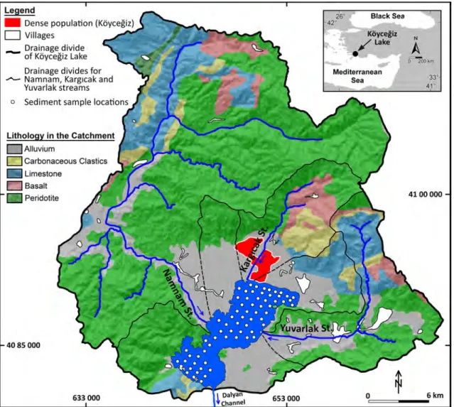
in the southwest of the Republic of Turkey (Fig. 1). The catchment area of Köyceğiz Lake (874 km2_{) comprises}

different lithological units: (1) Quaternary alluvium

(~ 170 km2_{), (2) carbonaceous clastics (~ 40 km}2_{), (3)}

limestone (~ 120 km2_{), (4) basalt (~ 44 km}2_{), and}

peri-dotite (~ 500 km2_{) (Fig. 1) (Şenel 1997). Mafic and}

ultra-mafic igneous rocks cover almost 60% of the Köyceğiz catchment area. Weathering products from the lithological units are carried into the lake by three main inlets, namely Namnam, Kargıcak and Yuvarlak streams. However, the lake is discharged into the Mediterranean Sea through the Dalyan Channel (Fig. 1). The study area includes subaque-ous and terrestrial hot and cold springs which affect the hydrogeochemical content of the aquatic systems (Avşar et al. 2017). Köyceğiz town (35,000 population) is the main settlement in the lake catchment. Citrus crops are the primary agricultural commodity and are farmed on Quaternary alluvium.

Fig. 1 Map showing the distribution of lithological units and settlements in the catchment of Köyceğiz Lake, as well as the sediment sampling locations within the lake (modified from Şenel 1997)

Legend

- Dense population (Koycegiz)

D

Villages

_ Drainage divide

of Koycegiz Lake Drainage divides for

-'"'- Namnam, Karg1cak and

Yuvarlak streams

Lithology in the Catchment

•

Alluvium

D

Carbonaceous Clastics 40 85 000 633 000 2s· 42• Black Sea Koycegiz /Lake

•

N

A

0 200km 33' 41° 4100000

Materials and methods

Fieldwork

The sediment core samples acquired in 2014 for this study were taken from boat using a gravity corer at 81 locations. The corer, consisting of a 50 cm-long PVC pipe, was left to free fall approximately 2 m above the sediment/water inter-face. Soon after the PVC pipe penetrated the sediments, the corer was extracted. A vacuum system, used with the corer, enabled the sediments to be kept in the PVC pipe. The sediment cores were a minimum of 10 cm in length. The cores were stored in a cooling room at 4 °C until they were submitted for ICP–MS analysis. Only the top 5 cm of the sediments was used for element concentration analyses. For this study, 81 sediment samples from Köyceğiz Lake were analyzed (Fig. 1). Sixty-seven of the 81 sample localities were distributed randomly across the study area; 14 samples were concentrated near the subaqueous hot springs (SUB-1, SUB-2 and SUB-3) in the south of the lake.

The use of a gravity coring system for this study (rather than an Ekman sampler) was important because the sedi-ment/water interface is not disturbed during gravity coring.

This allowed the most recent, age-equivalent sediments to be sampled and analyzed for element contamination.

Element analyses

Sample preparation was completed in the Fatsa Faculty of Marine Sciences Research and Laboratory Center. Eighty-one samples were completely desiccated at 105 °C in a furnace. Dried samples were ground in a porcelain mortar, and approximately 100 g of sediment was sieved through a 63 µm mesh (El-Said et al. 2014; Omar et al. 2015). The amount of material coarser and finer than 63 µm was meas-ured, and 2–3 g (min. 2 g) of material finer than 63 µm was separated for inductively coupled plasma–mass spectrometer (ICP–MS) analysis in an AQ270 packet (Acme Lab., Bureau Veritas Commodities Canada Ltd.).

The analysis of Mo, Cu, Pb, Zn, Ni, Co, Mn, Fe, As, Cd, Cr and Al elements was done using the ICP–MS method. Reference materials and duplicate measurements of three samples are presented in Table 1. Cd was not studied because the concentration of this element was below the detection limits of 0.5 ppm for Cd.

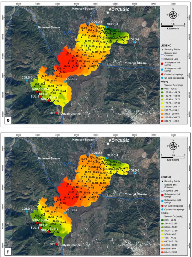
Table 1 _{Comparison of reference material values with measured values and measurement limits for elements}

Method AQ270 Analyte Mo Cu Pb Zn Ni Co Mn Fe As Cr Al Unit mg/kg mg/kg mg/kg mg/kg mg/kg mg/kg mg/kg % mg/kg mg/kg % MDL 0.5 0.5 0.5 5.0 0.5 0.5 5.0 0.0 5.0 0.5 0.0 Pulp duplicates  K27 Sediment pulp 8.0 35.5 10.7 48.0 697.8 49.7 573.0 3.1 < 5 197.8 1.2  K27 REP 8.5 35.3 10.5 52.0 699.6 51.9 551.0 3.1 < 5 195.6 1.2  K70 Sediment pulp 8.8 27.1 8.6 44.0 573.4 42.4 590.0 2.5 < 5 157.8 1.1  K70 REP 8.5 27.1 8.7 44.0 572.8 42.8 590.0 2.5 < 5 161.3 1.1  K-T-3-634 Sediment pulp 9.4 22.4 8.5 24.0 506.0 32.1 299.0 2.1 < 5 148.5 0.7  K-T-3-634 REP 9.2 21.0 8.1 23.0 484.9 29.5 291.0 2.0 < 5 141.0 0.6 Reference materials  STD GBM398-4-AR STD 929.6 3904.0 11945.5 5463.0 4217.6 2005.6 5261.0 3.9 6.0 1983.2 0.5  STD OREAS927-AR STD 0.9 11015.7 220.0 752.0 27.1 30.6 1026.0 8.0 12.0 40.9 3.2  STD GBM398-4-AR STD 948.3 4003.8 11895.2 5632.0 4225.4 2059.6 5285.0 3.7 6.0 2088.6 0.5  STD OREAS927-AR STD 1.1 11039.6 222.4 769.0 30.3 29.6 1009.0 8.1 13.0 42.5 3.3  STD GBM398-4-AR STD 940.7 3997.1 12043.1 5442.0 4256.1 2024.3 5311.0 3.9 6.0 2034.1 0.5  STD OREAS927-AR STD 1.1 10870.7 236.5 756.0 29.7 28.8 1049.0 8.0 14.0 41.0 3.3  STD GBM398-4-AR STD 927.6 3919.1 11747.9 5230.0 4180.6 2125.5 5240.0 3.9 7.0 2091.3 0.5  STD OREAS927-AR STD 1.0 10750.9 190.9 694.0 27.3 27.5 991.0 7.9 12.0 38.9 3.1  STD GBM398-4-AR STD 913.1 3968.7 11887.7 5462.0 4265.3 1975.3 5244.0 3.7 5.0 1966.0 0.5  STD OREAS927-AR STD 1.2 10869.0 231.2 761.0 28.9 28.7 1084.0 8.0 12.0 40.4 3.1  STD GBM398-4-AR (expected) 917.0 3919.0 11750.0 5345.0 4135.0 1950.0 5300.0 4.0 6.0 1950.0 0.48  STD OREAS927-AR (expected) 1.1 10715.0 232.0 726.0 30.9 29.4 1110.0 8.2 13.5 41.7 3.3

Ordinary kriging

To visualize the spatial distribution of elements in the study area, interpolation maps were created for the studied ele-ments utilizing a conventional Kriging method with the help of the Geostatistical Analyst module of ArcGIS 10.2.1 com-puter program. The interpolation maps were prepared using equal variogram parameters such as nugget effect, range and sill. Kriging surfaces are useful for showing the geographical distribution of anomalously high, moderate and low element concentrations.

Contamination analyses

Most of the techniques for element contamination evalua-tion compare the concentraevalua-tion of element in the modern sediments with the concentrations from the pre-industrial period. This type of evaluation can be used to assess anthro-pogenic influx of contaminants that are toxic to aquatic organisms. The contamination investigation techniques can be categorized into three groups as indicated by the pro-posed analysis methods; (1) those revealing the amount of anthropogenic pollution in sediments, (2) those investigat-ing the effect of sediment pollution on ecosystems and (3) those presenting the reference and/or limit values (Balik and Tunca 2015). The most widely used reference values are the ones presented by Turekian and Wedepohl (1961). The parameters and their calculation methods used to evaluate the element contamination in Köyceğiz Lake are presented below.

Contamination factor ( Ci f)

The contamination factor ( Ci

f ) was first introduced by

Hakanson (1980) to evaluate the anthropogenic element con-tamination in sediments. The method fundamentally makes a comparison between the present concentrations and the concentration of the reference baseline value of the pre-industrial time. Ci

f is calculated by Eq. 1, and ranges for C i f

classes are presented in Table 2.

where C_i is the amount of the element and C_n is the reference value of the element [average crustal abundance was used as a reference (Turekian and Wedepohl 1961)].

Contamination degree (Cd)

Contamination degree (Cd) was aslo presented by Hakanson (1980), and this strategy computes the anthropogenic ele-ment contamination in sediele-ments. This method sums the

(1)

Ci_f = Ci

C_n,

total element concentrations, and the formula for (Cd) is written below (Eq. 2). The ranges for Cd classes are also presented in Table 2.

where Ci_f is the contamination factor.

Modified contamination degree (mCd)

Abrahim and Parker (2008) modified the equation for con-tamination degree (C_d) by dividing the contamination degree by the quantity of the elements; using an average, the value is established using Eq. 3. The ranges for mCd classes are presented in Table 2.

where Ci_f is the contamination factor and n is the number

of elements analyzed.

Enrichment factor (EF)

The enrichment factor (EF) is another commonly utilized index for detecting anthropogenic element contamination in the sediments. This method aims at detecting the human effect on element contamination by taking elements such as Al and Fe as reference. Al and Fe are used as reference, since these elements are abundant in the aquatic environ-ment and less affected by contamination. Fe was utilized in this study as the reference element (Sallam et al. 2015; Zhu et al. 2017). The classification ranges for EF, which can be calculated with Eq. 4, are presented in Table 2.

where C_n is the quantity of the elements, C_ref is the value of the studied element in the reference sample (e.g., the Earth’s crust), Bn is the value of the reference element in the studied

sample (e.g., Fe or Al) and Bref is the value of the reference

element in the reference sample.

Geoaccumulation index (Igeo)

Another method used to evaluate the anthropogenic element contamination in the sediments calculates the geoaccumula-tion index (Igeo), which was initially proposed by Müller (1969). Igeo can be obtained using Eq. 5, and the ranges for the Igeo classes are presented in Table 2.

(2) Cd = n ∑ i=1 Cif, (3) mCd = ∑n i=1C i_f n , (4) EF = C_n C_ref B_n B_ref ,

Table 2 Scales sho wing t he le vels es tablished f or t he sediment assessment me thods used PEL pr obable effect le vel, TEL thr eshold effect le vel (Smit h e t al. 1996 ), ERM effect r ang e median, ERL effect r ang e lo

w (Long and Mor

gan 1991 ) Ear th cr us t’s v alues (T ur ekian and W edepohl 1961 ) Cu Pb Zn Ni As Cr ERM (fr eshw ater) 390 110 270 50 85 145 PEL (fr eshw ater) 197 91.3 315 36 17 90 TEL (fr eshw ater) 35.7 35 123 18 5.9 37.3 ERL (fr eshw ater) 70 35 120 30 33 80 Ear th ’s cr us t 45 20 95 68 13 90 Cont amination deg ree (Cd) Cont amination f act or ( C i)f Cd < 8 8 ≤ Cd ≤ 16 16 ≤ Cd ≤ 32 Cd ≥ 32 C i <f 1 1 ≤ C i <f 3 3 ≤ C i >f 6 C i≥ f 6 Low Moder ate Consider able Ver y high Respectiv ely lo w Moder ate Consider able Ver y high Modified cont amination deg ree (mCd) mCd < 1.5 1.5 ≤ mCd < 2 2 ≤ mCd < 4 4 ≤ mCd < 8 8 ≤ mCd < 16 16 ≤ mCd < 32 mCd ≥ 32 Nil t o v er y lo w Low Moder ate High Ver y high Extr emel y high Ultr a high Enr ic hment f act or (EF) EF < 2 2 ≤ EF < 5 5 ≤ EF < 20 20 ≤ EF < 40 EF ≥ 40 Minimal Moder ate Significant Ver y high Extr emel y high Geoaccumulation inde x (Ig eo) Ig eo ≤ 0 0 < Ig eo < 1 1 < Ig eo < 2 2 < Ig eo < 3 3 < Ig eo < 4 4 < Ig eo < 5 Ig eo ≥ 5 Pr acticall y uncont ami-nated Uncont aminated t o moder atel y Moder atel y Moder atel y t o s trong ly Str ong ly Str ong t o e xtr emel y Extr emel y

Pollution load inde

x (PLI) Po tential ecologic r isk f act or (ERi) 0 1 > 1 ERi < 40 40 ≤ ERi < 80 80 ≤ ERi < 160 160 ≤ ERi < 320 320 ≥ ERi Per fection Baseline De ter ior ation Low Moder ate Consider able High Ver y high m-PEL -Q m-ERM-Q m-PEL -Q < 0.1 0.1 < m-PEL -Q < 1 m-PEL -Q > 1 m-ERM-Q < 0.1 0.11 < m-ERM-Q < 0.5 0.51 < m-ERM-Q < 1.5 m-ERM-Q > 1.5 Unim pacted Moder atel y im pacted Highl y im pacted %9 t oxic %21 t oxic %49 t oxic %76 t oxic

where C_n is the quantity of the studied elements, B_n is the element concentration in the studied sample and 1.5 is the natural oscillation coefficient

Pollution loading index (PLI)

The pollution loading index (PLI), which can be calculated with Eq. 6, was introduced by Tomlinson et al. (1980) to com-pare the anthropogenic element contamination in sediments for different locations. The classification ranges for PLI can be found in Table 2.

where C_f is the contamination factor and n is the quantity of the studied elements.

Potential ecologic risk factor (ERi)

The potential ecologic risk factor, first utilized by Hakanson (1980), which can be calculated using Eq. 7, has been used to demonstrate the impact of element contamination on organ-isms and on ecosystems. The classification ranges for ERi can be found in Table 2.

where Ti_r is the toxic response factor, Ci is the amount of

element in samples and C0 is the reference value of the

element.

Mean effect range‑median quotient (m‑ERM‑q) and mean probable effect level quotient (m‑PEL‑q) methods

m-ERM-q and m-PEL-q indices are useful for understanding

the effect of element contamination in sediments on ecosys-tems using the effect range median (ERM) values and probable effect level (PEL) values (Table 2). The formulas are given below (Eqs. 8 and 9).

where C_i is the value of the studied element in the samples, ERM is the influence interval value of the studied element and N is the quantity of the studied elements.

(5) Igeo = log 2 ( _C n 1.5 × Bn ) , (6) PLI = (Cf 1 × Cf 2 × Cf 3 × … … Cfn)1n, (7) Eir =T i_{r × C}i Co , (8) m-ERM-Q = n ∑ i=1 C_i ERMi n , (9) m-ERM-Q = n ∑ i=1 C_i PELi n ,

where C_i is the value of the studied element in the samples, PEL is the average possible level of the effect value of the studied element and N is the quantity of the studied elements

Toxic unit sum (ΣTUs) and proportional toxic unit (proportional TU)

The toxic unit sum (ΣTUs) and proportional toxic unit (pro-portional TU) indices demonstrate the impact of the element contamination in sediments. The proportional TU can be calculated by using the values of ΣTUs. These indices are calculated by Eqs. (10 and 11).

where Ci is the amount of the studied element in the sam-ples, PELC_i is the PEL (probable effect level) value of the studied element and N is the quantity of the studied elements.

Statistical methods

Before comparison of the means and correlation analyses, the Shapiro–Willk test was used to identify the distribution of the data. This test is useful for evaluating small data sets (Aydin et al. 2014). Since the distribution was not paramet-ric, the Kruskal–Wallis test and Mann–Whintney U test from the comparison tests were utilized, and the Spearman correlation analysis was used as the correlation analysis method (Aydın et al. 2017). In cases where the data were insufficient to be identified as normally distributed, tests were used regardless of the distribution (Tunca et al. 2016). Cluster analysis (CA) was used after z-score correction via Euclidean distance according to the Ward method (Üçüncü Tunca et al. 2016). All statistical analyses were performed with SPSS v. 21 (IBM, USA).

Results and discussion

Current element level in the lake and intermetallic relationships

The coordinates of 81 sediment sampling locations and the results of ICP–MS analysis on these samples are pre-sented in Table 3. The results show that there are some differences between the areas of stream inlets and the (10) ∑ TUs = n ∑ i=1 C_i PELi , (11) Proportional TU = ⎛ ⎜ ⎜ ⎝ Ci PELi ΣTUs ⎞ ⎟ ⎟ ⎠ .

Table

3

ICP–MS anal

ysis r

esults of 81 sediment sam

ples # Sam ple ID X Y Mo (mg/ kg) Cu (mg/k g) Pb (mg/k g) Zn (mg/k g) Ni (mg/k g) Co (mg/k g) Mn (mg/ kg) Fe (%) Cr (mg/k g) Al (%) 1 K-1 648,955 4,090,607 5.4 49.0 11.7 64 675.7 51.0 653 3.69 199.3 1.67 2 K-2 648,150 4,089,979 7.5 37.6 12.2 52 644.0 48.8 693 3.09 189.2 1.30 3 K-3 646,262 4,087,710 2.2 46.8 8.2 53 1476.2 90.7 976 5.10 388.2 1.39 4 K-5 644,934 4,085,676 3.0 44.2 7.3 55 1278.1 79.4 850 4.68 391.4 1.34 5 K-6 643,321 4,084,181 8.0 26.1 7.6 36 648.9 38.9 362 2.49 194.8 0.87 6 K-7 642,862 4,083,653 8.1 25.0 6.9 30 554.2 34.9 314 2.20 165.2 0.80 7 K-9 642,097 4,083,621 7.7 24.5 6.3 29 604.1 33.4 267 2.34 167.0 0.81 8 K-10 643,798 4,083,413 12.3 27.8 9.6 37 535.4 34.4 338 2.13 170.3 0.80 9 K-11 644,188 4,084,101 3.3 29.3 8.9 43 812.6 62.6 1011 3.14 266.3 1.07 10 K-12 644,828 4,084,650 12.6 27.8 9.4 39 708.9 44.1 403 2.67 217.5 0.94 11 K-13 645,320 4,085,261 0.6 32.9 7.6 43 1002.7 66.4 922 3.45 295.2 0.94 12 K-14 645,876 4,085,956 0.0 41.3 6.7 52 1466.3 94.4 1185 4.67 371.1 1.09 13 K-15 646,450 4,086,636 0.0 41.0 7.0 52 1768.2 108.5 1003 5.40 439.8 1.11 14 K-16 646,992 4,087,300 1.0 42.5 7.0 54 1527.7 89.1 792 5.08 407.6 1.25 15 K-17 647,583 4,088,032 9.4 33.9 8.2 44 761.3 47.6 549 2.99 221.5 1.06 16 K-18 648,079 4,088,632 7.8 37.7 10.6 53 791.8 56.6 621 3.29 210.4 1.30 17 K-19 648,575 4,089,249 7.9 33.6 9.7 48 610.4 46.3 543 2.77 180.5 1.15 18 K-20 649,088 4,089,900 6.6 33.0 10.2 45 548.5 45.6 534 2.63 156.9 1.13 19 K-21 649,632 4,090,562 0.8 77.4 12.7 79 828.3 64.2 929 5.10 296.4 2.31 20 K-22 648,280 4,090,888 4.2 50.1 12.2 68 766.6 56.7 956 3.97 248.2 1.70 21 K-23 650,589 4,090,434 2.9 68.7 12.8 71 782.5 61.3 767 4.49 266.0 2.03 22 K-24 650,173 4,089,890 1.2 92.8 13.3 83 866.1 65.3 969 5.24 300.1 2.38 23 K-25 649,609 4,089,254 5.1 58.0 13.7 72 673.0 51.0 728 3.97 219.2 1.80 24 K-26 649,064 4,088,587 10.3 32.1 9.1 45 616.8 44.0 537 2.68 172.6 1.10 25 K-27 648,616 4,088,021 8.0 35.5 10.7 48 697.8 49.7 573 3.06 197.8 1.19 26 K-28 648,103 4,087,422 6.7 40.9 10.2 50 1062.5 68.1 690 3.92 286.1 1.26 27 K-29 647,464 4,086,657 1.9 42.9 8.8 53 1398.5 86.6 991 4.86 389.6 1.27 28 K-30 646,970 4,086,044 0.5 39.7 7.4 51 1716.7 109.2 1119 5.31 443.8 1.15 29 K-34 644,873 4,083,484 10.7 26.6 6.9 32 602.6 41.3 431 2.27 185.8 0.81 30 K-35 644,430 4,082,925 11.9 26.5 7.0 31 531.2 33.7 336 2.10 166.3 0.78 31 K-36 644,081 4,082,513 12.8 33.1 9.1 43 705.6 44.6 440 2.77 218.5 1.00 32 K-37 643,718 4,082,070 14.1 27.2 7.0 32 594.5 36.3 365 2.29 174.0 0.85 33 K-38 643,387 4,082,903 13.7 26.5 6.7 30 577.9 33.6 331 2.17 167.9 0.79 34 K-39 643,071 4,082,508 10.6 25.8 8.9 32 520.3 33.0 513 2.14 163.0 0.81 35 K-40 642,452 4,083,142 10.0 22.5 6.2 27 463.5 27.5 305 1.88 142.9 0.67 36 K-41 642,996 4,084,726 8.0 25.3 8.7 30 650.9 38.4 318 2.46 186.8 0.75

Table 3 (continued) # Sam ple ID X Y Mo (mg/ kg) Cu (mg/k g) Pb (mg/k g) Zn (mg/k g) Ni (mg/k g) Co (mg/k g) Mn (mg/ kg) Fe (%) Cr (mg/k g) Al (%) 37 K-42 644,494 4,081,634 7.1 25.9 10.2 37 548.6 34.4 446 2.31 192.4 0.88 38 K-43 644,872 4,082,142 5.0 23.0 7.1 29 475.3 28.1 405 1.89 149.7 0.74 39 K-44 645,379 4,082,750 4.5 26.9 7.7 32 607.4 39.7 483 2.49 195.1 0.96 40 K-47 648,001 4,086,000 0.0 25.3 7.6 41 919.7 63.9 2146 3.54 279.4 1.01 41 K-48 648,447 4,086,580 3.2 41.2 7.4 55 1209.7 78.6 1017 4.59 356.2 1.37 42 K-49 648,992 4,087,228 6.2 38.8 8.2 57 874.0 63.4 673 3.64 243.3 1.37 43 K-50 649,472 4,087,826 7.6 39.4 10.0 57 824.6 58.4 693 3.71 231.2 1.48 44 K-51 650,001 4,088,492 9.4 27.9 11.0 41 560.1 41.8 524 2.42 152.0 1.03 45 K-52 650,482 4,089,108 7.7 33.6 9.8 50 634.8 49.8 570 2.89 179.8 1.26 46 K-53 650,932 4,089,676 8.9 29.8 9.1 42 568.6 43.5 536 2.51 159.4 1.11 47 K-54 651,381 4,090,220 8.4 35.1 10.1 58 596.7 47.8 606 3.00 162.9 1.39 48 K-55 652,306 4,090,116 7.0 26.8 8.2 41 488.3 37.0 591 2.34 139.6 1.09 49 K-56 651,919 4,089,598 8.6 30.9 8.9 43 623.9 42.2 594 2.83 183.9 1.19 50 K-57 651,356 4,089,125 7.1 29.6 9.6 44 666.2 41.9 660 2.96 201.5 1.19 51 K-58 651,018 4,088,464 7.7 33.1 11.4 48 701.3 51.4 721 3.09 198.7 1.28 52 K-59 650,504 4,087,831 10.5 33.7 8.8 50 760.3 53.0 733 3.17 210.8 1.28 53 K-61 649,544 4,086,587 0.0 32.3 7.6 53 914.2 65.3 1519 4.15 273.5 1.43 54 K-62 649,048 4,085,973 0.0 19.4 6.6 32 647.1 42.9 1466 2.62 195.9 0.88 55 K-67 649,761 4,086,044 0.0 23.4 9.0 43 744.9 54.1 1637 3.29 221.9 1.12 56 K-68 650,723 4,087,255 0.0 27.7 9.7 48 850.2 61.9 2748 3.73 257.3 1.24 57 K-70 652,739 4,089,574 8.8 27.1 8.6 44 573.4 42.4 590 2.48 157.8 1.07 58 K-71 653,093 4,090,108 3.3 25.5 9.4 44 462.1 35.3 921 2.30 146.1 1.04 59 K-72 653,719 4,089,989 3.7 29.7 11.1 51 538.8 41.8 1215 2.68 185.1 1.19 60 K-73 653,410 4,089,703 5.7 24.8 9.8 43 470.3 36.2 687 2.19 147.7 0.99 61 K-74 653,614 4,089,248 2.6 29.8 11.0 48 560.4 45.4 1153 2.67 190.0 1.10 62 K-75 649,456 4,091,218 0.0 76.6 11.3 78 850.6 62.4 1075 5.25 295.5 2.28 63 K-76 650,035 4,091,048 3.7 69.1 15.1 80 759.0 57.6 834 4.70 267.1 2.10 64 K-77 650,813 4,090,888 4.2 34.1 11.0 56 472.5 36.4 684 2.86 153.3 1.40 65 K-78 651,312 4,090,737 0.8 65.8 24.9 116 205.1 30.4 800 4.67 98.5 2.73 66 K-79 651,919 4,090,534 2.2 41.6 15.0 73 322.2 33.5 736 3.18 114.2 1.78 67 K-80 652,488 4,090,455 4.3 29.7 9.6 49 419.6 34.5 823 2.61 139.3 1.26 68 K-R -027 643,975 4,081,886 9.8 31.7 7.5 44 623.8 43.8 472 2.59 201.5 1.09 69 K-R -618 644,120 4,081,843 10.5 29.5 7.4 38 611.2 39.2 429 2.52 197.2 1.04 70 K-R -619 643,861 4,081,923 10.4 25.6 6.5 34 512.0 30.9 353 2.14 166.2 0.91 71 K-R -620 643,987 4,082,011 7.2 16.2 5.1 34 354.0 22.6 249 1.49 108.2 0.52

rest of the lake in terms of the sediment element centrations. This difference is seen both in element con-centrations that accumulate in the sediment and in the interrelationships between metals. For this reason, the element concentrations in the sediments were evaluated separately for the entire lake and for four sub-regions, namely, at stream inlets including: (1) Namnam Stream mouth, (NamSM), (2) Kargıcak Stream mouth, (KarSM), (3) Yuvarlak Stream mouth (YuvSM) and (4) the south-western part of the lake where subaqueous hot springs are located (HotSR).

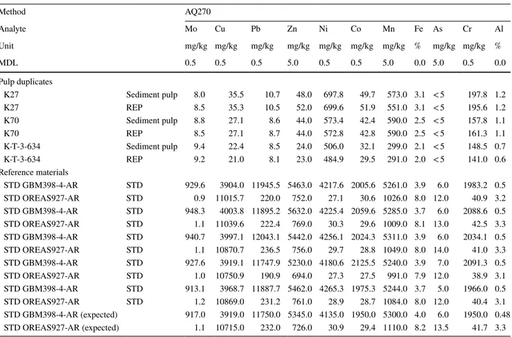
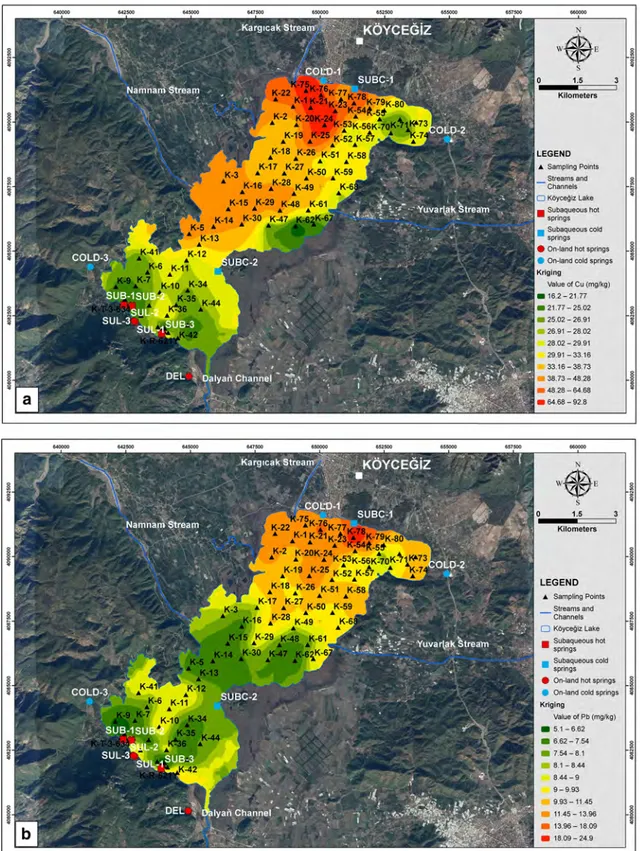
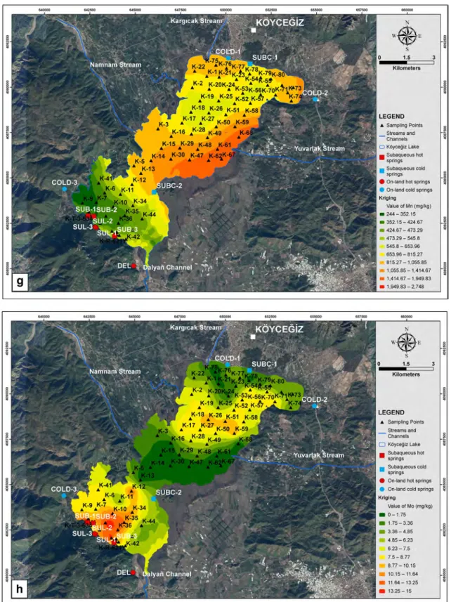
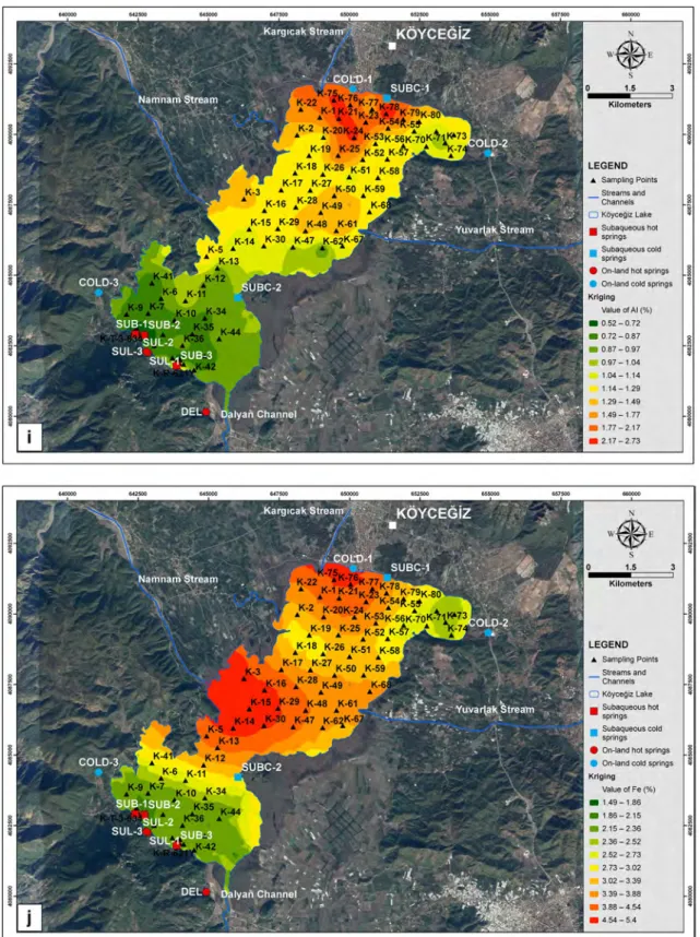
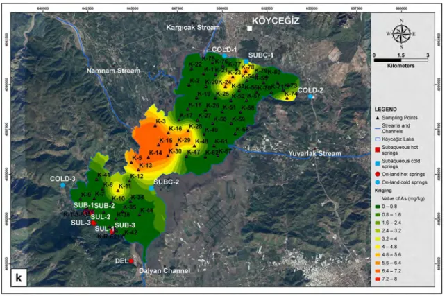
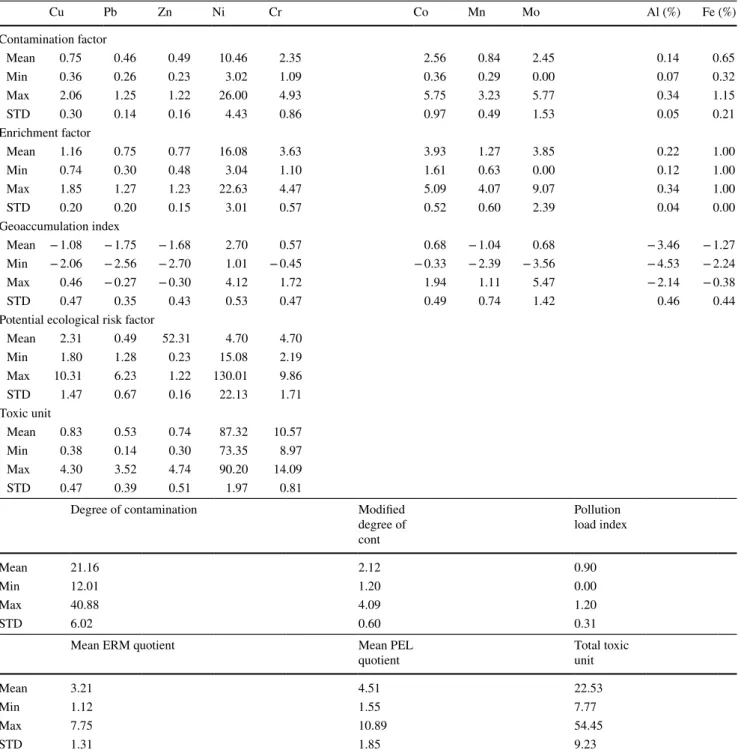
Kriged surfaces displayed on maps were used to show sediment element concentrations (Fig. 2a–j). In Table 4, descriptive statistics of elemental concentrations for the entire lake and the four sub-regions are presented. Accord-ingly, the region with the highest amount of elements accu-mulation in the lake is NamSM, followed by KarSM. Ele-ment concentrations in the sediEle-ments taken from YuvSM and HotSR are relatively low. The amount of mean elemental concentration for the entire lake is intermediate between the elemental concentration values in the four sub-regions. The sediment in Köyceğiz Lake has significantly higher concen-trations of Cr and Ni (Table 4). It is well known that the chemical weathering products of mafic and/or ultramafic rocks are expected to be rich in clay minerals, and elements such as Cr and Ni (e.g., Wronkiewicz and Condie 1989). Since peridotite and basalt cover almost 60% of the catch-ment of Köyceğiz Lake (Fig. 1), we attribute the source of high Cr and Ni concentrations in the sediments to the weath-ering of these rocks.

Sediment evaluation methods yield a similar picture. The degree of contamination (cd), modified degree of contamination (mCd) and pollution load index (PLI) were used to compare KarSM, NamSM, as well as the entire lake (Tables 5, 6, 7). These methods are commonly used to com-pare the general state of elements in multiple areas (Zhao et al. 2015; Alshahri 2017). Accordingly, the areas with the highest contamination indices are NamSM and KarSM, but the region that has higher contaminations varies accord-ing to the method used. Accordaccord-ing to Cd and mCd values, NamSM (34.09 and 3.41, respectively) is more contaminated than KarSM (21.45 and 2.15, respectively). These values put NamSM at a level of ‘very high contamination’ (yhe contamination scale is given on Table 2), which is the high-est value on the scale; KarSM at a level of ‘considerable contamination’, which is the second highest value on the scale. The reason why Cd gives such high results is largely due to the high contamination factor value of Ni. Since Cd is the sum of the contamination factor values of the elements being studied, Ni dominates the results. The arithmetic aver-age of Cd and mCd, on the other hand, reveals a slightly more optimistic picture. Since the high contamination factor value of Ni occurs in the arithmetic average, its predominant

Table 3 (continued) # Sam ple ID X Y Mo (mg/ kg) Cu (mg/k g) Pb (mg/k g) Zn (mg/k g) Ni (mg/k g) Co (mg/k g) Mn (mg/ kg) Fe (%) Cr (mg/k g) Al (%) 72 K-R -621-Y 643,940 4,081,750 4.7 26.3 10.0 54 635.6 44.0 1040 2.99 197.7 1.21 73 K-T-3-000 642,725 4,082,889 9.7 21.8 7.2 49 551.3 36.7 578 2.22 168.7 0.83 74 K-T-3-631 642,795 4,082,968 10.1 22.0 7.4 36 541.1 31.4 296 2.26 146.3 0.69 75 K-T-3-633 642,804 4,082,807 9.0 18.7 8.6 22 398.9 24.7 244 1.59 116.1 0.55 76 K-T-3-634 642,663 4,082,973 9.4 22.4 8.5 24 506.0 32.1 299 2.11 148.5 0.68 77 K-015-000 642,409 4,082,916 4.4 31.7 11.9 48 685.4 51.8 972 2.99 221.0 1.18 78 K-015-638 642,491 4,082,865 6.1 21.3 8.0 31 468.6 31.8 407 1.98 152.9 0.72 79 K-015-643 642,514 4,082,948 12.2 25.8 7.1 32 533.9 33.9 279 2.14 161.3 0.77 80 K-015-645 642,428 4,083,010 6.5 24.9 9.0 36 512.6 35.5 293 2.12 147.7 0.71 81 K-015-647 642,325 4,082,985 15.0 23.8 6.8 30 483.3 28.5 270 1.82 139.0 0.65

effect on the overall data is relatively small. According to the results of mCd, both regions are moderately contaminated.In the comparison based on PLI values, the results for NamSM

and KarSM are similar, but KarSM has a slightly higher value than NamSM (1.13 and 0.98, respectively). When we consider that the deterioration initiation value, which is the

Fig. 2 Spatial distribution of ten elements in the sediments of Köyceğiz Lake: a Cu, b Pb, c Zn, d Ni, e Cr, f Co, g Mn, h Mo, i Al and j Fe

-

N

w$e

_i

1.5 Kilometers

I

LEGENO • Sampling Points Slream:s and ! Cnann&ta 0 1<6)'«0~ Lake

'

• Subaqueous hot ,r,mg, • Sub:iiqueous cold spmgs • On-land hot sp,lngs I

• On-land cokl Spl'i\g.S

'

Krlglng Value

°'

Cu (mg/kg) e 16.2-21.77 • 21,77-25.02

I

• 25.02 -26.91 26.91 -28.02 28.02 -29.91 29.91 -33.16 33.16 -38.73 • 38.73-48.28 • 48.28 -64.68 • 64.68 - 92.8 N

W.

E

§ i 1.5 KIiometers

i

LEGEND

.A. Sampli"fg PO.,ts Streams.and Channels § D K4j,ceQiz Lake i • Subaqueous hot springs • Su~queous colel spnngs • On•land hol sprw'lgs _I • On•lsnd cokf spring, f Krlglng Vall.Je of Pb (mg/kg) a 5.1-6.62 - 6.62- 7.54 _§ • 7.54-e., _i 8.1-8.44 8.44 -9 9-9.93 9,93- 11.45 11.45 -13.96

i

a 13.96-18.09 - 18.09-24.9

Fig. 2 (continued)

-W*E

1.5 KIiometers

.& Samplf'lg PIX'lls Streams and Cnannels O K~iz.Lake 41.05-4•.15 44. 15-48.5 48.5-54,61 5o1.61 -63.2 Kilometers A Sampling Pe>inls Streams, andl Cl'ii11"1MIS 0 Kl)yQeQiz Loke 511.69-559,38 5!;9.38- 627.72 627 .72 - 725.65 725.65 -865.98 865.98 - 1,067.07

I

I

a i

I

I f

Fig. 2 (continued)

IV

.

. r

E

s 0 1.5 3 Kilometers LEGEND & Sampra,g P~IS

Streams and Channels 0 KOyce\)iz Lako • Su~queous h01 spongs • Su~queous cok:I springs • On.-l1;1nd hol 5-prrlgs.

• On.land cold sp,ings

Krlglng value or Cr {mg/kg) • 98.5 - 128.93 a 128.93- 149.74 a 1,49.74 -163.98 163.98-173.72 173.72-187.96 187 .96 -208. 77 208.77 -239.2 239.2 - 283.69 a 283.69-348.72 a 348. 72 - 443.8

...

N

IV

.

E

s 0 1.5 Kilometers LEGEND & Sampling Pmts Streams.and Charmels 0 KOyce,Qiz Ulke •

~~:eous

hot •

~~;eous

COICI • On-land hell splT!gs • Ona-land cold springs

Krtglng \lalue of Co (mg/kg) • 22.6 -29.43 a 29.43 - 33.6S • 33.6S -36.27 36.27- 37.B9 37.89-40.5 40.5-44.73 44.73-51.56 51.56 - 62.59 • 62.59- 80.41 • 80.41 -109.2 I

'

Fig. 2 (continued) ....,.

w@E

s 0 1.5 Kilometers LEGEND • S~pling Poinls Sl~msand CnannelS 0 KO'yeegiz La>:.e • Su~aqueous not spmgs • Subaqueous cold spmgs • On-land hot springs

• On-land cold spmgs Krlglng Vah.N!t of Mn (mg/kg) • 244-352.15 • 352.15 - 424.67 • 42-4.67 - 473.29 473.29 -545.8 545.8 -653.96 653.96- 815.27 815.27 -1,1155.85 1.055.a.5-1.414,67 • 1,414.67- 1,949.83 • 1.949.83-2,748 0 1.5 Kilometers LEGEND • Semplflg Posits Stt8ams and C~nnels 0 KOyc~lz Lake • ~~~~eoos hot • ~~~~eous cold e On-land hoi $pri1g.$ • On-land cold sp,ings

Kf'lglng Va~e ol Mo (mg/kg) a 0-1.75 a 1.75-3,36 a 3.36-4.85 4.85-6.23 6.23-7.5 7,5- 8,77 8.77-10.15 a 10.15-11.64 • 11.64-13.25 a 13.25-15

I

I

!

i

Fig. 2 (continued) LEGEND • sampling Points Streams and Channels 0 K0yc~il Lake • S.oaquoooshOI :spnngs • Subaqueous cold springs • On-land hot spmgs

• On-lend eold springs.

Krfglng vao.o of Al(%) • 0.52-0.72 • 0.72-0.87 • 0.87-0.97 0.97-1,04 t.04-1.14 1.14-1.29 1.29-1.49 t.49-1.77 • 1.77-2.17 • 2,17-2,73 """ N

W.

E

s 0 1.5 Kilometers LEGEND • Ssmpting Points Streams and Ch,emnels D K6ye<ijlz Lake • S.baqueous hol spnngs •

=:eouscold

• On-land hot spmgs • On-aaoo COid springs

Knglng va1ue ot Fll!I (%) • 1.49-1.86 • 1,86-2.15 a 2.15-2.36 2.36-2.52 2.52- 2.73 2.73-3.02 3.02-3.39 a 3.39-3.88 • 3.88-4.54 a 4,54-5.4

I

critical level for PLI = 1, the values obtained are at the upper limit. Similarly, the PLI value for the entire lake is 0.90, which indicates a severe contamination and at the upper limit of the contamination scale.

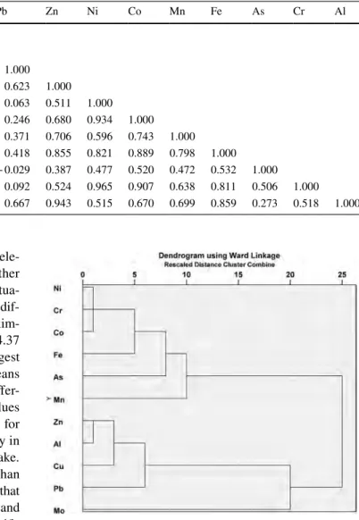
When we evaluated the general profile of the ten elements studied together with accumulation differences, it is seen that the strongest correlation is between Cr and Ni (r = 0.965) (Table 8). Other significant correlations were observed between Co and Ni (r = 0.934), and Cr and Co (r = 0.907). Strong correlations can also be seen between these elements on the kriged surface maps (Fig. 2a–j). Cluster analysis (CA) results are consistent with correlation analysis results. In the dendrogram, Ni, Cr and Co are in a single cluster and show the strongest relationship (Fig. 3). When we look at the distance proximity matrix of CA, it can be seen that the closest distances are between these three elements (Table 9): Cr–Ni (Euclidian distance = 2.10), Co–Ni (Euclidian dis-tance = 2.33), and Cr–Co (Euclidian disdis-tance = 2.43). The strong correlation between Cr, Co and Ni, and the accumu-lation levels in the sediments reveal the possibility of either an anthropogenic or rock (ultramafic) source, which is also supported by the EF values, with reference to the Earth crust values (Tables 5, 6, 7).

Cr–Co and Ni show elevated concentrations in lake sedi-ments when compared with crustal abundances (Tables 5, 6,

7). The contamination factor ( Ci

f ) values of these three

ele-ments (Ni = 20.45, Co = 4.58, Cr = 4.19) in NamSM are higher than in other parts of the lake. These values are ‘very high’ for Ni (Cfi ≥ 6), which is the highest value in the clas-sification, and ‘considerable’ (3 ≤ Cfi > 6) for Co and Cr. EF (Ni = 18.85, Co = 4.22, Cr = 3.86) and geoaccumulation index (Igeo) (Ni = 3.75, Cr = 1.47, Co = 1.59) results also support the Ci

fresults. Different scales are used in the

inter-pretation of the enrichment factor (EF). According to the first scale, a level of 1.5 indicates an anthropogenic source, and Ni, Co and Cr are well above this limit (Zhang and Liu

2002). In the five-stage scale developed by Haris and Aris, Ni shows strong accumulation, and Cr and Co show moder-ate accumulation (Haris and Aris 2012). According to the shown values, there is a strong contamination of Ni, which is the fifth level of the seven-level scale, and moderately contaminated for Co and Cr, which is the third level of the same scale (Tomlinson et al. 1980).

Another pair of elements with very high correlation values within the lake sediments is Al and Zn (Al–Zn

r = 0.943). The strong relationship between these two ments is also supported by cluster analysis. These two ele-ments were located in the same cluster in the cluster analysis (Fig. 3) and showed very close proximity in the proximity matrix with an Euclidian distance of 2.47 (Table 9). This is the second closest distance after the Cr–Ni–Co triple. When

Fig. 2 _(continued) I~ . Namnam Stream \, SUB-1SUB-2 SUL-2 SUL-3 SUL-1SUB-3

:~

,:.

i.l~/

-

·-

·

•

. ·.

· .. Yuvarlak_'Stream

W

.

. r

E

§ s i 0 1.5 Kilometers

I

LEGEND • Sampffng Polnls Streams and § Channers _i 0 K&fceOlz Lake • Subaqueous hot sprtngs • Su~aqueous cold >l)Ollgs I

• On-land hot :!ipting:!i

• On-land cold springs f

KrljJlng Value ot As (mg/kg) a 0-0.8 ao.a-1.s § • 1.6-2.4 i 2.4 -3.2 3.2-4 4-4,8 4.8-5.6 5.6-6.4 • 6.•-7.2 • 7.2-8

Table 4 The v alues of t he s tudied elements, t he limit v alues of t

hese elements accor

ding t

o sediment q

uality guidelines and t

he com par ison of t hese v alues of t he s tudied elements Ther e is no s tatis tical significance be tw een t he line and t he superscr ip t le tters ( p < 0.05) Mo (mg/k g) Cu (mg/k g) Pb (mg/k g) Zn (mg/k g) Ni (mg/k g) Co (mg/k g) Mn (mg/k g) Fe (%) As (mg/k g) Cr (mg/k g) Al (%) Entir e lak e (a)  Mean 6.30 d,e 34.38 e 9.29 b,d,e 46.93 e 712.81 c 48.88 c 713.35 3.09 e 1.30 c,d,e 212.45 c,e 1.17 b,e  S td 3.99 14.10 2.72 15.49 301.29 18.44 418.66 1.02 2.56 77.55 0.43  Min 0.00 16.20 5.10 22.00 205.10 22.60 244.00 1.49 0.00 98.50 0.52  Max 15.00 92.80 24.90 116.00 1768.20 109.20 2748.00 5.40 8.00 443.80 2.73 Namnam S tream mout h (N amSM) (b)  Mean 2.08 c,e 42.05 7.84 a,d,e 52.00 e 1366.61 85.25 940.20 c,e 4.69 c 6.30 371.34 1.24 a,e  S td 1.99 3.92 1.05 3.50 230.84 12.60 136.60 0.59 0.67 47.84 0.15  Min 0.00 32.90 6.70 43.00 1002.70 66.40 690.00 3.45 5.00 286.10 0.94  Max 6.70 46.80 10.20 55.00 1768.20 108.50 1185.00 5.40 7.00 439.80 1.39 K ar gıcak S tream mout h (K arSM) (c)  Mean 2.63 b,e 64.91 14.27 78.40 672.91 a,e 53.34 a,e 844.70 b,e 4.43 b 2.00 a,d,e 230.45 a,e 2.08  S td 1.92 15.52 3.94 14.45 226.84 12.32 132.63 0.70 3.27 73.32 0.35  Min 0.00 41.60 11.30 64.00 205.10 30.40 653.00 3.18 0.00 98.50 1.67  Max 5.40 92.80 24.90 116.00 866.10 65.30 1075.00 5.25 8.00 300.10 2.73 Ho t spr ing ar ea (Ho tSR) (d)  Mean 8.71 a,e 23.87 8.45 a,b,e 36.20 531.67 35.04 467.80 2.22 1.10 a,c,e 159.92 0.80  S td 3.36 3.58 1.57 10.82 81.57 7.80 300.17 0.45 2.33 30.02 0.22  Min 4.40 18.70 6.80 22.00 398.90 24.70 244.00 1.59 0.00 116.10 0.55  Max 15.00 31.70 11.90 54.00 685.40 51.80 1040.00 2.99 6.00 221.00 1.21 Yuv ar lak S tream mout h (Y uvSM) (e)  Mean 4.57 a,b,c,d 31.18 a 8.98 a,b,d 47.62 a,b 792.85 c 55.88 c 1162.08 b,c 3.37 a 0.38 a,c,d 230.88 a,c 1.23 a,b  S td 4.11 6.47 1.45 7.29 169.22 10.80 695.06 0.61 1.39 52.57 0.18  Min 0.00 19.40 6.60 32.00 560.10 41.80 524.00 2.42 0.00 152.00 0.88  Max 10.50 41.20 11.40 57.00 1209.70 78.60 2748.00 4.59 5.00 356.20 1.48 Sediment q uality guidelines  PEL 197.00 91.30 315.00 36.00 90.00  ERM 390.00 110.00 270.00 50.00 145.00  TEL 35.70 35.00 123.00 18.00 37.30  ERL 70.00 35.00 120.00 30.00 80.00

Table 5 Sediment assessment me thods r esults f or t he K ar gıcak S tream r egion (K arSM) f or t he elements s tudied Cu Pb Zn Ni Cr Co Mn Mo Al (%) Fe (%) Cont amination f act or  Mean 1.44 0.71 0.83 9.90 2.56 2.81 0.99 1.01 0.26 0.94  Min 0.92 0.57 0.67 0.35 1.09 1.60 0.77 0.00 0.21 0.68  Max 2.06 1.25 1.22 12.74 3.33 3.44 1.26 2.08 0.34 1.12  S TD 0.34 0.20 0.15 3.34 0.81 0.65 0.16 0.74 0.04 0.15 Enr ichment f act or  Mean 1.84 0.91 1.05 12.60 3.26 3.58 1.27 1.17 0.33 1.20  Min 1.18 0.72 0.86 3.84 1.39 2.04 0.98 0.00 0.27 0.86  Max 2.63 1.59 1.59 16.22 4.25 4.38 1.61 2.65 0.43 1.42  S TD 0.44 0.25 0.19 4.25 1.04 0.83 0.20 0.92 0.06 0.19 Geoaccumulation inde x  Mean − 0.09 − 1.11 − 0.88 2.60 0.68 0.86 − 0.61 − 0.74 − 2.55 − 0.69  Min − 0.70 − 1.41 − 1.15 1.01 − 0.45 0.09 − 0.97 − 2.29 − 2.85 − 1.15  Max 0.46 − 0.27 − 0.30 3.09 1.15 1.20 − 0.25 0.47 − 2.14 − 0.43  S TD 0.35 0.33 0.24 0.70 0.58 0.39 0.23 1.10 0.24 0.24 Po tential ecological r isk f act or  Mean 7.21 3.57 0.83 49.48 5.12  Min 4.62 2.83 0.67 15.08 2.19  Max 10.31 6.23 1.22 63.68 6.67  S TD 1.72 0.99 0.15 16.68 1.63 To

xic unit  _Mean

1.71 0.96 1.44 84.11 11.78  Min 1.03 0.45 0.88 73.35 10.27  Max 4.30 3.52 4.74 87.04 14.09  S TD 0.94 0.95 1.22 3.95 0.97 Deg ree of cont amination Modified deg ree of cont

Pollution load inde

x Mean 21.45 2.15 1.13 Min 12.22 1.22 0.00 Max 26.12 2.61 1.43 ST D 4.94 0.49 0.43 Mean ERM q uo tient Mean PEL q uo tient To tal t oxic unit Mean 3.13 4.40 21.99 Min 1.12 1.55 7.77 Max 4.01 5.65 28.27 ST D 1.00 1.42 7.08

the values of Al and Zn in the lake sediment were compared with the Earth crust values, accumulation levels in the sedi-ment were found to be very low. It is difficult to suggest an anthropogenic effect for these two elements because the EF value obtained based on the Earth crust reference is very low (Tables 5, 6, 7). This means that the strong relationship between these elements is of lithological origin. Similarly, it can be seen in the literature that Al and Zn demonstrate very strong correlations without exceeding the Earth crust val-ues. Another interesting point between these two elements that draws our attention is that they are both concentrated in

KarSM. In the sediment samples in this area, significantly higher levels of Al and Zn were detected compared to the lake in general and other important areas.

Copper was also evaluated. In particular, Cu content of the sediment samples near KarSM, which contain more Cu than the entire lake (Table 4), resulted in higher Ci

f values

(Cu = 1.44) (Tables 5, 6, 7). According to the EF values (Cu = 1.84), an enrichment in Cu occurs. In addition, Igeo with a value of 2.60 is ranked at level 4 on the seven-level scale and indicates a moderate to strong contamination level. When we look at the elements that are most strongly

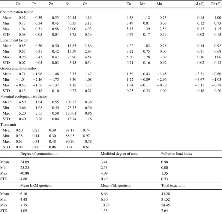
Table 6 Sediment assessment method results for Namnam Stream region (NamSM) for the elements studied

Cu Pb Zn Ni Cr Co Mn Mo Al (%) Fe (%) Contamination factor  Mean 0.92 0.39 0.55 20.45 4.19 4.58 1.12 0.73 0.15 1.00  Min 0.73 0.34 0.45 0.35 3.18 3.49 0.81 0.00 0.12 0.73  Max 1.04 0.51 0.58 26.00 4.93 5.75 1.39 2.58 0.17 1.15  STD 0.08 0.05 0.04 3.75 0.59 0.77 0.17 0.79 0.02 0.13 Enrichment factor  Mean 0.85 0.36 0.50 18.85 3.86 4.22 1.03 0.78 0.14 0.92  Min 0.67 0.31 0.42 13.59 2.93 3.22 0.75 0.00 0.11 0.68  Max 0.96 0.47 0.47 23.96 4.54 5.30 1.28 3.09 0.16 1.06  STD 0.07 0.05 0.03 3.45 0.54 0.71 0.16 0.92 0.02 0.12 Geoaccumulation index  Mean − 0.71 − 1.96 − 1.46 3.75 1.47 1.59 − 0.43 − 1.45 − 3.31 − 0.60  Min − 1.04 − 2.16 − 1.73 3.30 1.08 1.22 − 0.89 − 2.96 − 3.67 − 1.03  Max − 0.53 − 1.56 − 1.37 4.12 1.72 1.94 − 0.11 − 0.29 − 3.11 − 0.38  STD 0.13 0.18 0.10 0.27 0.21 0.25 0.23 1.09 0.18 0.20

Potential ecological risk factor

 Mean 4.59 1.94 0.55 102.25 8.38  Min 3.66 1.68 0.45 73.73 6.36  Max 5.20 2.55 0.58 130.01 9.86  STD 0.40 0.26 0.04 18.74 1.18 Toxic unit  Mean 0.50 0.21 0.39 89.17 9.74  Min 0.38 0.14 0.30 88.03 8.97  Max 0.63 0.34 0.48 90.20 10.78  STD 0.08 0.06 0.06 0.74 0.61

Degree of contamination Modified degree of cont Pollution load index

Mean 34.09 3.41 0.98

Min 25.25 2.53 0.00

Max 40.88 4.09 1.35

STD 4.86 0.49 0.53

Mean ERM quotient Mean PEL quotient Total toxic unit

Mean 6.16 8.66 43.28

Min 4.48 6.30 31.52

Max 7.75 10.89 54.45

correlated with Cu, it can be seen that these are Al and Zn, and Cu forms a strong correlation with these elements (Cu–Al = 0.88, Cu–Zn = 0.87) (Table 8). These correlations are also supported by CA (Table 9; Fig. 3). It can also be seen that these elements are introduced to the lake in signifi-cant amounts through the Kargıcak Stream. When we con-sider that the source of these two elements within the lake is natural based on sediment evaluation methods (Tables 5, 6,

7), and EF values in particular, the high concentration of Cu

may not be anthropogenic despite its high EF values. It is known that EF gives high values when elements from natural sources produce high values in sediments (Lar and Gusikit

2015). Considering the relationships between these three elements derived from Kargıcak Stream inlet, a common natural source is more likely than a possible anthropogenic source.

Among our findings, perhaps the most important were the molybdenum results. Mo was not only the single element

Table 7 Sediment assessment methods results for the entire Köyceğiz Lake for the elements studied

Cu Pb Zn Ni Cr Co Mn Mo Al (%) Fe (%) Contamination factor  Mean 0.75 0.46 0.49 10.46 2.35 2.56 0.84 2.45 0.14 0.65  Min 0.36 0.26 0.23 3.02 1.09 0.36 0.29 0.00 0.07 0.32  Max 2.06 1.25 1.22 26.00 4.93 5.75 3.23 5.77 0.34 1.15  STD 0.30 0.14 0.16 4.43 0.86 0.97 0.49 1.53 0.05 0.21 Enrichment factor  Mean 1.16 0.75 0.77 16.08 3.63 3.93 1.27 3.85 0.22 1.00  Min 0.74 0.30 0.48 3.04 1.10 1.61 0.63 0.00 0.12 1.00  Max 1.85 1.27 1.23 22.63 4.47 5.09 4.07 9.07 0.34 1.00  STD 0.20 0.20 0.15 3.01 0.57 0.52 0.60 2.39 0.04 0.00 Geoaccumulation index  Mean − 1.08 − 1.75 − 1.68 2.70 0.57 0.68 − 1.04 0.68 − 3.46 − 1.27  Min − 2.06 − 2.56 − 2.70 1.01 − 0.45 − 0.33 − 2.39 − 3.56 − 4.53 − 2.24  Max 0.46 − 0.27 − 0.30 4.12 1.72 1.94 1.11 5.47 − 2.14 − 0.38  STD 0.47 0.35 0.43 0.53 0.47 0.49 0.74 1.42 0.46 0.44

Potential ecological risk factor

 Mean 2.31 0.49 52.31 4.70 4.70  Min 1.80 1.28 0.23 15.08 2.19  Max 10.31 6.23 1.22 130.01 9.86  STD 1.47 0.67 0.16 22.13 1.71 Toxic unit  Mean 0.83 0.53 0.74 87.32 10.57  Min 0.38 0.14 0.30 73.35 8.97  Max 4.30 3.52 4.74 90.20 14.09  STD 0.47 0.39 0.51 1.97 0.81

Degree of contamination Modified

degree of cont Pollution load index Mean 21.16 2.12 0.90 Min 12.01 1.20 0.00 Max 40.88 4.09 1.20 STD 6.02 0.60 0.31

Mean ERM quotient Mean PEL

quotient Total toxic unit

Mean 3.21 4.51 22.53

Min 1.12 1.55 7.77

Max 7.75 10.89 54.45

with significant negative correlation among all studied ele-ments, but also showed negative correlation with all other elements (Table 8). CA results also fully support this situa-tion. In the dendrogram, Mo is also clearly separated in a dif-ferent cluster from all other elements (Fig. 3). In the proxim-ity matrix, its distance to other elements ranges from 14.37 to 16.73 Euclidian distances. These values are the largest for distance among all the elements (Table 9). This means that the source of Mo’s accumulation in the lake is differ-ent from the source of other elemdiffer-ents. However, EF values indicate Mo enrichment in the lake. Interpolation maps for Mo (Fig. 2h) show that the area with the highest density in the lake is the in-lake water source located south of the lake. Statistically, this area contains significantly more Mo than the areas NamSM and KarSM (Table 4). Despite the fact that it contains more Mo than the area near Yuvarlak Stream and the lake in general, this difference is not statistically signifi-cant. Groundwater sources can carry large quantities of Mo (Wang et al. 2016; Jones 2017). Based on these findings, it is clear that the factor constituting a significant proportion of Mo in lake sediments is a groundwater source located to the south.

Based on our findings, Pb, As, Mn and Fe do not pose an environmental risk. These elements are within the limit values for all values analyzed, and do not behave differently across the lake.

Environmental impact of the current element levels in the lake

The effect of current element concentrations in the lake on living organisms was investigated near stream inlets, water inflows and the entire lake using different methods. According to the sediment quality guidelines, there are two elements that could pose a threat to the lake. These are Ni and Cr. Both elements have values above all crite-ria (Table 4). Although Ni is an essential micronutrient for the metabolism of some aquatic organisms, it is also

toxic in high concentrations (Bielmyer et al. 2013). More-over, it is also not clear whether Ni is essential for animals (Blewett and Leonard 2017). Rocks, volcanic activity and forest fires are natural sources of Ni, coal and oil fumes, wastewater, electroplating, cement and steel industry activity, and phosphate-containing fertilizers all contain Ni (Savorelli et al. 2017). The toxic characteristics of Ni emerge in five different ways: (1) disruption of Ca2+

homeostasis, (2) disruption of Fe2+/3+ _{homeostasis, (3)}

ROS-induced oxidative damage, (4) disruption of Mg2+

homeostasis and (5) allergic response of respiratory epi-thelia. These pathways manifest themselves in three dif-ferent ways: (1) reducing the availability of Ca2+ _required

for exoskeleton, shell and bone formation, (2) respira-tory disturbance and (3) cytotoxicity and tumor formation (Brix et al. 2017). Cr is found naturally in rocks, soil and volcanic emissions; anthropogenic sources of Ni include

Table 8 Correlation matrix of

the studied elements Mo Cu Pb Zn Ni Co Mn Fe As Cr Al

Mo 1.000 Cu − 0.409 1.000 Pb − 0.258 0.539 1.000 Zn − 0.561 0.874 0.623 1.000 Ni − 0.446 0.614 0.063 0.511 1.000 Co − 0.571 0.724 0.246 0.680 0.934 1.000 Mn − 0.823 0.543 0.371 0.706 0.596 0.743 1.000 Fe − 0.682 0.863 0.418 0.855 0.821 0.889 0.798 1.000 As − 0.490 0.434 − 0.029 0.387 0.477 0.520 0.472 0.532 1.000 Cr − 0.493 0.619 0.092 0.524 0.965 0.907 0.638 0.811 0.506 1.000 Al − 0.537 0.880 0.667 0.943 0.515 0.670 0.699 0.859 0.273 0.518 1.000

Fig. 3 _{Cluster analysis (CA) dendrogram showing the relationships}

between the elements studied in the sediments of Köyceğiz Lake Ni Cr Co Fe As Zn Al cu Pb Mo 0 ~

Oendrogram using Ward Linkage Retcalod Distance Clusler Combine

10 15 I I -

-LJ

~

-20 25

alloys and coatings, stainless steel production in the auto-motive sector, nuclear and high-temperature research, and paint and metallurgical industries (Vaiopoulou and Gikas

2012). Despite its role in carbohydrate metabolism as part of the glucose tolerance factor, it is associated with cardi-ovascular risks and some metabolic syndromes (Bilandžić et al. 2017). The presence of a toxic effect or the nature of the toxic effect depends on the concentration and valence. Although its valence can vary between − 2 and + 6, it is mostly found in nature in its most stable forms of + 3 and + 6 valence. Of these forms, + 6 is more toxic and is the non-essential form with higher dissolution properties (Ergul-Ulger et al. 2014).

Toxic unit results indicate that Ni has the highest envi-ronmental risk factor for the lake (Tables 5, 6, 7). Ni alone makes up 87% of the total toxic effect in the lake. This rate is 84% in KarSM and 89% in NamSM. Accord-ing to the total toxic unit values, the area where the toxic effect is most apparent is NamSM, with a value of 43, and the area with the lowest toxic effect is HotSR with a value of 17. The mean effect range-median quotient (m-ERM-q) and mean probable effect level quotient (m-PEL-q) val-ues were used separately on lake sediments for different regions, to understand the toxic effect rate of element accumulation on living organisms. These results also sup-port total toxic unit results. According to m-ERM-q and m-PEL-Q values, the area with the highest toxic effect on living organisms is NamSM, and the area with the least toxic effect is HotSM. However, all m-ERM-q and m-PEL-Q values in terms of both the regional analysis and for the entire lake show toxic effects at the top of their scales. The rate of impact according to m-ERM-q is over 76%. According to m-PEL-q values, all regions are at a “highly impacted” level.

Although Cd was also studied in the lake, it was at concentrations below the limits of detection, and there-fore they were not included in the tables. The findings of

previous studies at different locations can also be seen in Table 10.

Conclusion

The sediment element accumulation levels, relationships between the accumulated elements and the effects on the ecosystem have been investigated in Köyceğiz Lake, both in sub-regions and across the entire lake. Multivariate statistical techniques, sediment assessment methods and interpolation maps were effective tools in understanding the contamination in the lake.

The results show that the highest level of element is found in the sediment samples taken from the area near Namnam and Kargıcak stream inlets, and the lowest ele-ment concentrations were found in the area where there are in-lake groundwater sources. According to sediment assessment methods, these two regions have the highest contamination level and the degree of contamination in these regions varies between the upper–intermediate and the highest levels, while showing some differences based on the methods used. Average lake element concentrations are low compared to other inlet areas, although the lake sediments still show element contaminations. The sources of the high contamination values observed in the lake were determined to be primarily Ni and to some extent Cr. These two elements, particularly in the area where Nam-nam Stream flows into the lake, are above the limit values for the lake, and this creates contamination throughout the lake. Ni and Cr were found to be highly statistically correlated. Apart from these two elements, there is no sig-nificant element contamination in the lake. When the effect of existing element accumulation on the ecosystem was evaluated, the two different methods used gave the highest toxic effect values.

Based on these findings, we can conclude that in-depth studies should be carried out in the lake for Ni and Cr, but

Table 9 Proximity matrix of the cluster analysis performed on the studied elements

Mo Cu Pb Zn Ni Co Mn Fe As Cr Al Mo 0.00 Cu 15.27 0.00 Pb 14.37 7.79 0.00 Zn 15.69 4.70 5.57 0.00 Ni 15.46 10.30 13.94 11.25 0.00 Co 16.04 9.16 12.81 9.83 2.33 0.00 Mn 16.73 11.15 11.61 10.15 9.65 8.67 0.00 Fe 16.49 5.64 10.11 6.32 5.98 4.55 8.64 0.00 As 15.49 9.90 11.66 9.93 7.51 7.29 10.82 7.73 0.00 Cr 15.84 9.24 13.38 10.45 2.10 2.43 9.11 4.98 7.36 0.00 Al 15.63 3.64 5.90 2.47 11.42 10.01 10.15 6.29 10.64 10.47 0.00

Table

10

Com

par

ison of me

tal accumulation indices in t

he sediments of K öy ceğiz Lak e wit h pr evious s tudies Mo Cu Pb Zn Ni Co Mn Fe As Cr Al

Abu Khashaba coas

tline, Egyp t Cf NA 0.52 18.80 1.84 6.69 3.62 0.64 2.22 22.59 0.00 NA El sor ogy e t al. ( 2016 ) EF NA 0.26 10.60 0.79 3.16 1.93 0.36 NA 12.64 0.00 NA Ig eo NA − 1.61 3.23 0.72 2.11 1.27 − 1.21 0.41 3.91 − 5.96 NA Koumoundour ou Lak e, Gr eece Ig eo NA 2.58 0.61 2.68 − 0.20 NA NA NA 1.69 3.56 NA Hahladakis e t al. ( 2013 ) Nor th-w es ter n par t of Elef sis Ba y, Gr eece Ig eo NA − 0.22 0.61 1.29 − 0.52 NA NA NA 1.14 2.16 NA Outer par t of İzmir Ba y, T ur ke y EF NA 0.51 NA 1.35 1.24 NA 0.58 1.15 NA NA NA Kont as ( 2008 ) Inner par t of İzmir Ba y, T ur ke y EF NA 0.93 NA 2.55 1.36 NA 0.54 1.2 NA NA NA Ther maik os Gulf, Gr eece EF NA 2.9 5.1 1.7 NA NA NA NA NA NA NA Chr ist ophor idis e t al. ( 2009 ) Homa Lagoon, T ur ke y Cd 7.07 (A ver ag e v alue) Ulutur han e t al. ( 2011 ) Cf NA 0.41 0.53 0.75 1.25 NA 0.66 0.5 NA 1.14 0.32 Edk u Lak e, Ey gp t PLI 4.6 El-Said e t al. ( 2014 ) RI 68.8 Cd 48 mCd 6.9 Candar li Gulf, T ur ke y Cd 11.68 (a ver ag e v alue) Pazi ( 2011 ) Cf NA 1.06 1.37 1.52 0.89 NA 1.49 NA 1.12 0.99 NA Lang at Riv er , Mala ysia EF NA 1.94 9.45 5.95 NA NA NA NA 80.53 NA NA Shafie e t al. ( 2012 ) Ig eo NA − 1.48 0.23 − 0.2 NA NA NA NA 2.24 NA NA Kö yceğiz Lak e, T ur ke y Cf 0.78 1.45 1.13 1 1.24 1.3 1.11 1.23 NA 1.24 1.27 Cur rent s tudy (a ver ag e v alue) EF 0.65 1.18 0.97 0.83 1.01 1.06 0.89 1 NA 1.01 1.04 Ig eo 1.94 − 0.13 − 0.46 − 0.65 − 0.38 − 0.29 − 0.63 − 0.36 NA − 0.36 − 0.32 Cd 11.74 mCd 1.17 PLI 0.93

most importantly Ni. In these studies, it is of utmost impor-tance that the source of these elements be clearly deter-mined, and the status of accumulation in living organisms, especially those living in the sediments, be revealed.

Acknowledgements This study was supported by The Scientific and

Technological Research Council of Turkey (TÜBİTAK, Project Num-ber 112Y137) and by the Muğla Sıtkı Koçman University funds (Pro-ject Number BAP16/150).

References

Abrahim GMS, Parker RJ (2008) Assessment of heavy metal enrich-ment factors and the degree of contamination in harbor sedienrich-ments from Tamaki Estuary, Auckland, New Zealand. Environ Monit Assess 136:227–238

Alexakis D (2011) Diagnosis of stream sediment quality and assess-ment of toxic eleassess-ment contamination sources in East Attica, Greece. Environ Earth Sci 63:1369–1383

Alshahri F (2017) Heavy metal contamination in sand and sediments near to disposal site of reject brine from desalination plant, Ara-bian Gulf: assessment of environmental pollution. Environ Sci Pollut Res 24:1821–1831

Avşar Ö, Avşar U, Arslan Ş, Kurtuluş B, Niedermann S, Güleç N (2017) Subaqueous hot springs in Köyceğiz Lake, Dalyan Channel and Fethiye-Göcek Bay (SW Turkey): locations, chemistry and origins. J Volcanol Geotherm Res. https ://doi. org/10.1016/2017.07.016

Aydin M, Karadurmuş U, Tunca E (2014) Biological characteristics of

Pachygrapsus marmoratus in the southern Black Sea (Turkey). J

Mar Biol Assoc U K 94:1441–1449

Aydın M, Tunca E, Alver Şahin Ü (2017) Effects of anthropological factors on the metal accumulation profiles of sea cucumbers in near industrial and residential coastlines of İzmir, Turkey. Int J Environ Anal Chem 97:368–382

Bakan G, Özkoç HB (2007) An ecological risk assessment of the impact of heavy metals in surface sediments on biota from the mid-Black Sea coast of Turkey. Int J Environ Stud 64:45–57 Balık İ, Tunca E (2015) A review of sediment contamination

assess-ment methods. Turk J Marit Mar Sci 1:37–47

Bielmyer GK, DeCarlo C, Morris C, Carrigan T (2013) The influence of salinity on acute nickel toxicity to the two euryhaline fish spe-cies, Fundulus heteroclitus and Kryptolebias marmoratus. Envi-ron Toxicol Chem 32:1354–1359

Bilandžić N, Tlak Gajger I, Kosanović M, Čalopek B, Sedak M, Solo-mun Kolanović B, Varenina I, Luburić ĐB, Varga I, Đokić M (2017) Essential and toxic element concentrations in monofloral honeys from southern Croatia. Food Chem 234:245–253 Blewett TA, Leonard EM (2017) Mechanisms of nickel toxicity to fish

and invertebrates in marine and estuarine waters. Environ Pollut 223:311–322

Brix KV, Schlekat CE, Garman ER (2017) The mechanisms of nickel toxicity in aquatic environments: an adverse outcome pathway analysis. Environ Toxicol Chem 36:1128–1137

Christophoridis C, Dedepsidis D, Fytianos K (2009) Occurrence and distribution of selected heavy metals in the surface sediments of Thermaikos Gulf, N. Greece. Assessments using pollution indica-tors. J Hazard Mater 168:1082–1091

El-Said GF, Draz SE, El-Sadaawy MM, Mooner AA (2014) Sedimen-tology, geochemistry, pollution status and ecological risk assess-ment of some heavy metals in surficial sediassess-ments of an Egyptian

lagoon connecting to the Mediterranean Sea. J Environ Sci Health A Tox Hazard Subst Environ Eng 49:1029–1044

El-Sorogy AS, Tawfik M, Almadani SA (2016) Assesment of toxic metals in coastal sediments of the Roestta area, Mediterranean Sea, Egypt. Environ Earth Sci 75:398

Ergul-Ulger Z, Ozkan AD, Tunca E, Atasagun S, Tekinay T (2014) Chromium(VI) biosorption and bioaccumulation by live and acid-modified Biomass of a Novel Morganella morganii Isolate. Sep Sci Technol 49:907–914

Eziz M, Mohammad A, Mamut A, Hini G (2018) A human health risk assessment of heavy metals in agricultural soils of Yanqi Basin, Silk Road Economic Belt, China. Hum Ecol Risk Assess 24:1352–1366

Hahladakis J, Smaragdaki E, Vasilaki G, Gidarakos E (2013) Use of sediment quality guidelines and pollution indicators for the assess-ment of heavy metal and PAH contamination in Greek surficial sea and lake sediments. Environ Monit Assess 185:2843–2853 Hakanson L (1980) An ecological risk index for aquatic pollution

con-trol. A sedimentological approach. Wat Res 14:975–1001 Haris H, Aris AZ (2012) The geoaccumulation index and enrichment

factor of mercury in mangrove sediment of Port Klang, Selangor, Malaysia. Arab J Geosci 6:4119–4128

He Z, Song J, Zhang N, Zhang P, Xu Y (2009) Variation characteristics and ecological risk of heavy metals in the south Yellow Sea sur-face sediments. Environ Monit Assess 157:515–528

Ismail Z, Beddri A (2009) Potential of water hyacinth as a removal agent for heavy metals from petroleum refinery effluents. Water Air Soil Pollut 199(1):57–65

Joksimovic D, Tomic I, Stankovic AR, Jovic M, Stankovic S (2011) Trace metal concentrations in Mediterranean blue mussel and sur-face sediments and evaluation of the mussels quality and possible risks of high human consumption. Food Chem 127:632–637 Jones SA (2017) Geology and geochemistry of fault-hosted

hydrother-mal and sedimentary manganese deposits in the Oakover Basin, east Pilbara, Western Australia. Aust J Earth Sci 64:63–102 Kinimo KC, Yao KM, Marcotte S, Trokourey A (2018) Distribution

trends and ecological risks of arsenic and trace metals in wetland sediments around gold mining activities in central-southern and southeastern Côte d’Ivoire. J Geochem Explor 190:265–280 Kontas A (2008) Trace metals (Cu, Mn, Ni, Zn, Fe) Contamination

in Marine Sediment and Zooplankton Samples from Izmir Bay (Aegean Sea, Turkey). Water Air Soil Pollut 188:323–333 Kusin FM, Azani NNM, Hasan SNMS, Sulong NA (2018) Distribution

of heavy metals and metalloid in surface sediments of heavily-mined area for bauxite ore in Pengerang, Malaysia and associated risk assessment. Catena 165:454–464

Lar UA, Gusikit RB (2015) Environmental and health impact of poten-tially harmful elements distribution in the Panyam (Sura) vol-canic province, Jos Plateau, Central Nigeria. Environ Earth Sci 74:1699–1710

Long ER, Morgan LG (1991) The potential for biological effects of sediment-sorbed contaminants tested in the National Status and Trends Program. NOAA Technical Memorandum NOS OMA 52. National Oceanic and Atmospheric Administration, Seattle, p 175 Müller G (1969) Index of geoaccumulation in sediments of the Rhine

River. Geo J 2:108–118

Nobi EP, Dilipan E, Thangaradjou T, Sivakumar K, Kannan L (2010) Geochemical and geo-statistical assessment of heavy metal con-centration in the sediments of different coastal ecosystems of Andaman Islands, India. Estuar Coast Shelf Sci 87:253–264 Omar MB, Mendiguchía C, Er-Raioui H, Marhraoui M, Lafraoui G,

Oulad-Abdellah MK, García-Vargas M, Moreno C (2015) Dis-tribution of heavy metals in marine sediments of Tetouan coast (North of Morocco): natural and anthropogenic sources. Environ Earth Sci 74:4171–4185

Pazi I (2011) Assessment of heavy metal contamination in Candarli Gulf sediment, Eastern Aegean Sea. Environ Monit Assess 174:199–208

Rahman MS, Saha N, Molla AH (2014) Potential ecological risk assessment of heavy metal contamination in sediment and water body around Dhaka export processing zone, Bangladesh. Environ Earth Sci 71:2293–2308

Ridgway J, Shimmield G (2005) Estuaries as repositories of historical contamination and their impact on shelf seas. Estuar Coast Shelf Sci 55:903–928

Sallam AS, Usman ARA, Al-Makrami HA, Al-Wabel MI, Al-Omran A (2015) Environmental assessment of tannery wastes in relation to dumpsite soil: a case study from Riyadh, Saudi Arabia. Arab J Geosci 8:11019–11029

Sany SBT, Salleh A, Sulaiman AH, Sasekumar A, Rezayi M, Tehrani GM (2013) Heavy metal contamination in water and sediment of the Port Klang coastal area, Selangor, Malaysia. Environ Earth Sci 69:2013–2025

Savorelli F, Manfra L, Croppo M, Tornambè A, Palazzi D, Canepa S, Trentini PL, Cicero AM, Faggio C (2017) Fitness evaluation of Ruditapes philippinarum exposed to Ni. Biol Trace Elem Res 177:384–393

Şenel M (1997) Geological Map Series of Turkey 1:100 000 scale.No. 1, Geologic Map of Fethiye L7 Quadrangle.General Directorate of Mineral Research and Exploration. Geological Research Depart-ment, Ankara (in Turkish)

Shafie NA, Aris AZ, Zakaria MP, Haris H, Lim WY, Isa NM (2012) Application of geoaccumulation index and enrichment fac-tors onthe assessment of heavy metal pollution in the sedi-ments. J Environ Sci Health A Toxic/Hazard Subst Environ Eng 48:182–190

Smith SL, Macdonald DD, Keenleyside KA, Ingersoll CG, Field LJ (1996) A preliminary evaluation of sediment quality assessment values for freshwater ecosystems. J Great Lakes Res 22:624–638 Tomlinson DL, Wilson JG, Harris CR, Jeffrey DW (1980) Problems in

the assessment of heavy-metal levels in estuaries and the forma-tion of a polluforma-tion index. Helgolander Meeresunters 33:566–575 Tunca E, Aydın M, Şahin ÜA (2016) Interactions and accumulation

differences of metal(loid)s in three sea cucumber species collected from the Northern Mediterranean Sea. Environ Sci Pollut Res 23:21020–21031

Turekian KK, Wedepohl KH (1961) Distribution of the Elements in some major units of the Earth’s crust. Geol Soc Am Bull 72:175–192

Üçüncü Tunca E, Ölmez TT, Özkan AD, Altındağ A, Tunca E, Tekinay T (2016) Correlations in metal release profiles following sorption by Lemna minor. Int J Phyto 18:785–793

Uluturhan E, Kontas A, Can E (2011) Sediment concentrations of heavy metals in the Homa Lagoon (Eastern Aegean Sea): assess-ment of contamination and ecological risks. Harbor Pollut Bull 62:1989–1997

Vaiopoulou E, Gikas P (2012) Effects of chromium on activated sludge and on the performance of wastewater treatment plants: a review. Wat Res 46:549–570

Wang D, Xia W, Lu S, Wang G, Liu Q, Moore WS, Arthur Chen CT (2016) The nonconservative property of dissolved molybdenum in the western Taiwan strait: relevance of submarine groundwater discharges and biological utilization. Geochem Geophys Geosyst 17:28–43

Wronkiewicz DJ, Condie KC (1989) Geochemistry and provenance of sediments from the Pangola Supergroup, South Africa: evidence for a 3.0 Ga-old continental craton. Geochim Cosmochim Acta 53:1537–1549

Wu SS, Yang H, Guo F, Han RM (2017) Spatial patterns and origins of heavy metals in Sheyang River catchment in Jiangsu, China based on geographically weighted regression. Sci Total Environ 580:1518–1529

Zhang J, Liu CL (2002) Riverine composition and estuarine geochem-istry of particulate metals in China—weathering features, anthro-pogenic impact and chemical fluxes. Estuarine Coast Shelf Sci 54:1051–1070

Zhang C, Shan B, Tang W, Dong L, Zhang W, Pei Y (2017) Heavy metal concentrations and speciation in riverine sediments and the risks posed in three urban belts in the Haihe Basin. Ecotoxicol Environ Saf 139:263–271

Zhao R, Coles NA, Wu J (2015) Status of heavy metals in soils follow-ing long-term river sediment application in plain river network region, southern China. J Soils Sediments 15:2285–2292 Zhu L, Liu J, Xu S, Xie Z (2017) Deposition behavior, risk assessment

and source identification of heavy metals in reservoir sediments of Northeast China. Ecotoxicol Environ Saf 142:454–463