Labor migration and trade patterns in the presence of age composition differences across countries: an overlapping generations analysis

?r г-'

-J

^,- ^ W S i f e i j t ΰ ϊ 1 ¿ “^ % ^ i : b â . 2 € ü „ N -2 ^ â f§ ^ .-Л fe_ ^ sT- '^· ^ y'·---- :" ■' fSirJbÿ'ç' “· · ' V;

LABOR MIGRATION AND TRADE PATTERNS IN THE PRESENCE OF AGE COMPOSITION DIFFERENCES

ACROSS COUNTRIES:

AN OVERLAPPING GENERATIONS ANALYSIS

The Institute o f Economics and Social Sciences of

Bilkent University

by

ALÎ EMRE UYAR

In Partial Fulfillment of the Requirements for the Degree of MASTER OF ARTS IN ECONOMICS

m

THE DEPARTMENT OF ECONOMICS BILKENT UNIVERSITY

ANKARA

Н 6 145^

■

I certify that I have read this thesis and have found that it is fully adequate, in scope and in quality, as a thesis for the degree of Master o f Arts in Economics.

Assistant Professor Dn Serdar Sayan Supervisor

I certify that I have read this thesis and have found that it is fully adequate, in scope and in quality, as a thesis for the degree o f Master o f Arts in Economics.

Assistant Professor Dr. Erdem Başçı Examining Committee Member

I certify that I have read this thesis and have fotmd that it is fully adequate, in scope and in quality, as a thesis for the degree o f Master o f Arts in Economics.

Dr. Neil Amwine

Examining Committee Member

Approval of the Institute o f Economics and Social Sciences

Professor Dr. Ali Karaosmanoglu Director

ABSTRACT

LABOR MIGRATION AND TRADE PATTERNS IN THE PRESENCE OF AGE COMPOSITION DIFFERENCES

ACROSS COUNTRIES:

AN OVERLAPPING GENERATIONS ANALYSIS

Uyar, All Emre

M.A., Department o f Economics Supervisor: Assist. Prof Dr. Serdar Sayan

September 2000

This study examines various effects of population growth differentials across countries by using a two country overlapping generations (OLG) general equilibrium model and shows that the resulting differences in age composition o f populations provide not only a basis for trade but also incentives for international migration of labor. The analysis starts by considering autarky equilibria of the countries that are assumed to be identical except for population growth rates initially, and shows that the country with the lower (higher) population growth rate will have higher (lower) capital per worker, wage rate and lifetime utility at all times. The cases of free trade and international mobility o f labor are then simulated for a comparative investigation.

The simulations with the considered migration scheme reveal that the steady state value o f migration rate equalizes the post-migration population growth rates in both coimtries. When trade is also taken into consideration, the results indicate that the country that is attractive to the migrants would prefer trade to migration, if it is a large country relative to the other. If both countries are equal in size, on the other hand, trade turns out to be Pareto-inferior to migration for the host country, with autarky being Pareto-superior to both trade and migration.

Keywords : Overlapping Generations, General Equilibrium, Age Composition Differences, Migration, Trade.

ÖZET

ÜLKELER ARASI YAŞ KOMPOZİSYONU

FARKLILIKLARI DURUMUNDA İŞGÜCÜ GÖÇÜ VE TİCARETİN YÖNÜ: BİR EŞANLI NESİLLER ANALİZİ

Uyar, Ali Emre

Yüksek Lisans, İktisat Bölümü Tez Y öneticisi: Yrd. Doç. Dr. Serdar Sayan

Eylül 2000

Bu çalışma, ülkeler arası nüfus büyüme farklannm çeşitli etkilerini, iki ülkeli bir eşanlı nesiller genel denge modeli çerçevesinde incelemekte ve bu farklann sonucu olarak nüfüslann yaş kompozisyonlan arasında oluşan eşitsizliğin hem ticaret, hem de uluslararası işgücü göçü için temel oluşturduğunu göstermektedir. Analiz, başlangıç anında nüfus artış oranlan dışında birbirinin tıpatıp aynı koşullarla karşı karşıya olan iki ülke ekonomisinin zaman içindeki değişimini, birbiriyle temas etmedikleri durumdan yola çıkarak yapılmaktadır. Kurulan model, daha sonra, serbest ticaret ve uluslararası işgücü hareketlerini de gözönüne alacak biçimde simule edilmiş ve değişik senaryolardan elde edilen sonuçlar karşılaştınimıştır.

İncelediğimiz göç simulasyonlan, göç oranlannm durgun hal değerlerinin göç-sonrası nüfus artış oranlannı eşitlediğini göstermektedir. Ticaret de göz önüne alındığında, göçmen işgücü için çekici olan ülkenin diğerine göre büyük ülke olması durumunda, fiilen göç almak yerine ticareti tercih ettiği görülmektedir. Öte yandan, iki ülkenin eşit büyüklükte olması halinde ev sahibi ülke için göç, ticarete kıyasla Pareto-baskm çıkmakta; buna karşın, kapalı ekonomi durumu hem ticaret hem de göçmen kabulüne Pareto-baskm olmaktadır.

Anahtar Kelimeler : Eşanlı Nesiller, Genel Denge, Yaş Kompozisyonu Farklan, Göç, Ticaret.

ACKNOWLEDGEMENTS

I would like to express my gratitude, first and foremost, to Professor Serdar Sayan for his guidance and the invaluable intellectual and moral support he provided during the entire course of this study. He has been a great supervisor. Thanks to his understanding and patience, we were able to maintain our relaxed attitude and sense o f humor even as we go over the sixth draft o f this thesis, one week before I leave for the U.S. with a list o f things to do as thick as this thesis.

I would like to thank also to the members o f my examination committee. Professors Erdem Başçı and Neil Amwine, for their really insightful comments and suggestions, from which I truly benefited a great deal.

I am, and will forever be, indebted to Ayça Kaya for her everlasting support during the most challenging years o f my life. Without her, this thesis would have never been finished. I would also like to thank each one o f my class and officemates for the extremely kind and joyful atmosphere they created. Their fnendship turned my tenure at Bilkent Economics Department into an unforgettable experience.

Last but certainly not least, I am grateful to my family for being so supportive, patient and understanding.

TABLE OF CONTENTS ABSTRACT ... iii ÖZET ... iv ACKNOWLEDGMENTS ... v TABLE OF CONTENTS ... vi CHAPTER I: INTRODUCTION ... 1

CHAPTER II: LITERATURE REVIEW... 4

CHAPTER III: THE CASE OF AUTARKY ... 12

3.1 The Model ... 12

3.1.1 Production Sector ... 14

3.1.2 Household’s Problem ... 17

3.1.3 Solving the Model ... 18

3.2 The Results ... 19

CHAPTER IV: MIGRATION ... 25

4.1 Migration Scenario 1 ... 26

4.2 Migration Scenario 2 ... 30

CHAPTER V: TRADE ... 32

CHAPTER VI: CONCLUSION ... 39

REFERENCES ... 46

APPENDICES A. POPULATION GROWTH RATE, AGE COMPOSITION AND

n

... 49

B. TRADE SCENARIO 2 ... 50

CHAPTER 1

INTRODUCTION

Population aging in developed coimtries and its possible economic consequences have attracted considerable attention in the previous decade. Aging o f the baby-boom generations, coupled with declining fertility rates o f new generations, causes dramatic changes in the demographic structures o f these countries. Projections by United Nations show that the average share o f the elderly (over 65) population in OECD countries will double in the next 50 years. Possible consequences o f such substantial increases in dependency ratios include variations in the values o f many economic variables such as labor supply, saving rates, real wages, returns to capital and hence, capital per worker, along with their implications on public pension and health care systems.

The likely consequences o f this transition have been explored by many researchers, such as Auerbach et al. (1989), Hviding and Merette (1998), Ken9 and

Sayan (2000), Fougere and Merette (1999), with somewhat diverging results on the extent o f various effects. Aside from these, the decline in young to old ratios in the populations o f developed countries and the resulting increase in wages and living standards is expected to induce labor migration out o f the developing countries. While this is already an important issue (for example between USA and Mexico, the EU and surrounding countries, in particular Turkey), the current demographic trend is likely to increase pressures for increased mobility o f labor across borders in the future.

The first aim o f this thesis is to explore the role o f differences in age compositions and growth o f population rates in neighboring nations as a possible source o f migration. For this purpose, we consider two economies that are initially the same in every aspect except for the population growth rate and show that this alone is enough to induce differences in wage rates and utilities, thereby providing incentives for workers from a country to migrate to another. The model we use is a 2- country, infinite horizon, OLG model with 2 goods and 2 factors o f production (capital and labor).

Our next aim is to model a migration scheme and investigate its effects on both countries by placing a special emphasis on finding a steady state value for the migration rate. We also compare the steady state in each country with and without migration.

A related issue that we address concerns the relationship between trade and migration, which is indeed an old and well debated subject. As R.J. Ruffin (1984, p. 266) puts it:

...Heckscher (1919), Meade (1951), Lemer (1952), Samuelson (1949), and many others have suggested that trade is a substitute for factor movements. The basis for this suggestion is the factor endowment theory o f international trade pioneered by Ohlin and Heckscher...

...W hen factor price equalization holds [Lemer (1952), Samuelson (1949)], trade is a perfect substitute for factor movements.

Yet, there is ample evidence that developed countries heavily favor free trade over free migration o f labor.’ We investigate possible reasons underlying the behavior of developed countries by incorporating free trade into our model, and then comparing results (especially the welfare implications for the host country) across the scenarios with free movement of labor and free trade.

The plan o f the thesis is as follows: Chapter 2 contains a literature review. Chapter 3 describes the model and reports simulation results for both countries under the autarky conditions. Chapter 4 and 5 discuss trade and migration scenarios, respectively, and present findings. Comparison o f different scenarios and concluding remarks are presented in Chapter 6.

^ Wellish and Walz (1998) and Razin and Sadka (1995) propose a justification for this behavior, by showing that the migration can actually be more costly to the host country.

CHAPTER 2

LITERATURE REVIEW

The effects o f population aging on various economic variables, especially those related to social security, have been the focus o f many studies starting from the previous decade. The initial studies in the area such as Hagemann and Nicoletti (1989) employed partial equilibrium methods or used projections that ignore the demographically induced changes in many related variables, such as real wages.

Auerbach and Kotlikoff (1987) developed a dynamic computable general equilibrium OLG model to study the effects o f population aging, as well as numerous other economic phenomena. Based on life-cycle theory o f saving behavior, their model investigated rational responses o f households to perfectly foreseen changes in current and future wages, interest and tax rates by allowing for 55 overlapping generations to be alive in any given period within the model horizon. Later, Auerbach et. al. (1989) slightly modified this model to allow for 75 overlapping generations and introduced bequest behavior, technological change, endogeneity of government expenditures with respect to age composition o f the population and open economy features to study the effects of projected demographic changes in the United States, Japan, Germany and Sweden over the 1985-2050 period. Their simulations showed that, as population ages, the consumption tax rates and national saving rates would decline in all countries, while the social security contribution rates and real wages would increase. Their main finding is that the studies that do not use general equilibrium models overestimate the burden o f population aging by

ignoring the effects of the increase in real wages. However, the effects o f population aging on national saving rates, real wage rates and current accounts as well as the possible welfare costs and the problems regarding the distribution across cohorts remain significant even in a general equilibrium framework.

Auerbach and Kotlikoff (1987) model was later modified in many directions to capture more realistic features of economies tmder consideration. Perraudin and Pujol (1991), for example, incorporated open economy features with 2 different kinds (export and non-tradeable) goods into the Auerbech-Kotlikoff framework; Broer et al (1994) introduced probability o f dying; Ken9 and Sayan (2000) extended

the model to investigate demographic shock transmission. Hyving and Merette (1998) and Fougere and Merette (1999). Hyving and Merette (1998) used an Auerbach and Kotlikoff (1987) type model to study the effects o f population aging in seven OECD covmtries in the period between 1954-2082. Their results are similar to that o f Auerbach-Kotlikoff (1987) and suggest substantial increases in wage income tax rates and decreases in capital per worker, real return on capital, national saving rate and real output per capita. Fougere and Merette (1999) modified this model to include endogenous human-capital formation. Their results show that investment in human capital offsets some o f the effects o f population aging in the long-run, even reversing the effect in the case of real output per capita.

A formal treatment o f the two-sector OLG models is relatively (and surprisingly) new. While models that include two or more sectors have been used sparingly since Calvo (1978) and Reichlin (1986) who used models with fixed- proportions production technologies to investigate some local properties o f 2 sector OLG models, Galor (1992) was the first to formally develop a 2-sector OLG model

and establish conditions to ensure the existence and uniqueness o f a perfect foresight equilibrium path. In Galor (1992), one of the goods is used for consumption only while the other is being used only as capital. The households that live for 2 periods get utility from consuming the consumption good and buy the other good only for investment purposes. The investment good that is produced in a period is then used as the capital stock of the next period. Galor (1992) shows that under certain assumptions,^ there exists a globally unique perfect-foresight equilibrium.

Extensions o f Galor (1992) model include Farmer (1997) and Guillo (1999). Farmer (1997) modifies the model to include heterogenous capital and static price expectations o f agents. Guillo (1999) uses the Galor (1992) type production and capital formation to investigate the effect o f relative factor intensities on the relationship between the terms of trade and the capital stock. The study shows, contrary to a common result in the literature, that, under certain conditions, an import sector growing faster than the export sector is not required for a country’s terms of trade and capital per worker to move in the same direction.

The literature on migration is vast and diverse addressing such issues as incentives for migration, welfare effects o f migration on both countries, comparison o f temporary and permanent migration, comparison o f migrants and native workers, etc. Here, we mainly concentrate on the studies that use general equilibrium OLG models, a part o f the literature led by numerous contributions by Oded Galor.

^ Assumptions regarding the production and utility functions may be satisfied by many well-behaving functions. Additional assumptions include investment good being capital intensive, old age consumption being a normal good and savings increasing with increasing real interest rate.

Calor (1986) establishes a 2-factor OLG model with two countries that are exactly the same in every aspect, except for the time preferences o f their residents. The main results o f the paper can be summarized as:

(1) Depending on whether the countries imder or over invest with respect to the golden rule level, the difference in time preferences across countries may induce labor migration from one country to another or even bilateral migration. Calor (1986, p. 1) explains it as : “ ...labor migrates from the high (low) to the low (high) time preference country if both countries under (over) invest relative to the Golden Rule.”^

(2) The comparison of wages in both countries are rmaffected by migration. More specifically, wages in the source country remain at its autarky level while the wage rate in the host country always stays above that value. Therefore, the incentive to migrate persists even after the start o f migration, resulting in the migration o f whole population o f one country migrating to the other.

(3) As a result o f the international labor migration, the natives o f the host country are made worse off (in terms o f lifetime utility) while the non-migrants in the source country are at least as well off.

The last result is particularly important since it is contradicting with the results in classical trade theory (Heckscher-Ohlin) which requires that international

^ As explained in Karayalcin (1999), this means migration from impatient country to the patient country if both countries are dynamically efficient.

factor movements (which are thought to be substitutes o f international trade) benefit both of the participating countries.

Karayalcin (1999) uses the same model as Galor (1986) to study temporary migration, i.e., the workers migrate in the first period o f their lives and turn back in the second period. He concludes that the wages in both countries are affected from such a migration, resulting in a steady state which does not require the whole population o f a country to migrate to the other. The welfare effects on both countries remain the same as Galor (1986). Karayalcin (1999) also modifies the Galor (1986) model to contain an immobile factor of production (land) which again results in a steady state migration rate that is less than 1 implying that not all the workers in a country migrate to the other.

On the other hand, Geide (1998) consideres two countries, one o f which depends on personal savings while the other one uses a social security system, and concludes that this may provide incentives for migration. These incentives also remain on the long run, causing the migration o f whole population o f a country to the other.

Other studies about migration using OLG models include Galor and Stark (1991), which use a similar model to show that incentives to migrate can arise from a difference in the countries’ level of technology instead o f time-preferences as in Galor (1986), and Kochhar (1992) which endogenizes labor-leisure choice in the Galor (1986) model.

Galor and Stark (1990, 1991), also using OLG frameworks, attribute a positive value to the probability of migrants’ return home. The probability o f return migration provides incentives for migrants to save more and work more (as result o f their intertemporal utility maximization) than the natives o f the host country. When the ex-ante probability o f return is not realized, the migrants end up with a higher income than the natives, thereby explaining why migrants usually are more successful economically than native-boms in real life. Chiswick (1986a, 1986b) show that this is indeed the case for the U.S.

Djajic and Milbome (1988) and Djajic (1989) also use the approach of taking workers as utility-maximizing individuals who solve intertemporal utility maximization problems to make their decision about migration and length of their stay abroad, while Ethier (1985) and Rivera-Batiz (1983) deal with temporary migration in a guest-worker system.

As explained in the introduction section, the substitubility o f international trade and international factor movements is a result o f the factor price equalization property o f the fundamental Hecksher-Ohlin model. This is suggested by many researchers such as Ohlin (1929), Heckscher (1919), Meade (1951), Lemer (1952), Samuelson (1949). Since then, factor-price equalization has been critisized on various grounds and it is has been argued in such as Markusen (1983) and Wong (1995) that trade and migration are complements rather than substitutes. Razin and Sadka (1997) compare different trade models that result in either substitution or complementarity between trade and labor mobility and explain the key features of models that are responsible for contradicting results.

Some studies show that the host country in an international migration scheme may prefer trade even if the factor price equalization holds. Wellisch and Walz (1997) argue that one feature that from missing in the Hecksher-Ohlin framework is the existence o f the modem welfare state and this may cause underestimation o f costs o f migration to the host country. Their results indicate that existence of redistributional policies lower the level of social welfare for the host country. Developed countries typically prefer free trade over free labor migration, since the former allows them to enjoy gains of integration via trade without taking the burden o f welfare decreasing effects caused by redistribution policies in the latter.

Razin and Sadka (1995) emphasize the same point by showing that when the migrants are allowed to benefit from various services o f the welfare state, the cost of migration o f unskilled labor to the host country may exceed the gains from migration for that country, thereby providing an anti-migration factor. They also argue that another anti-migration factor may result from rigidity o f wages at the host country by showing that influx o f unskilled labor may lower the total share o f native workers in such a case.

The main contribution o f this thesis is to show that age composition differences among countries suffice to provide incentives for international labor migration. Establishing this result in an overlapping generations framework is the first in the literamre to the best of our knowledge. Some o f our results, such as the welfare implications of migration, are in line with the previous studies that explore migration using OLG models. Although incentives to migrate do remain in the long run, the steady state level o f migration serves to equalize the states o f countries without resulting the migration of whole population o f one country to the other,

contrary to Galor (1986) and Geide (1998). Incorporation o f free trade features to the model enables us to compare free migration with free trade from the perspective o f a developed country and we conclude, like Razin and Sadka (1995) and Wellisch and Walz (1997), that preferring free trade over accepting migrants can be justified.

CHAPTER 3

THE CASE OF AUTARKY

In this section, we describe the model under the assumption that there are no interactions between countries and concentrate on the behavior o f certain variables that belong to a single country. Since our main concern is the effects o f differences in age compositions resulting from differing population growth rates across countries, we consider values that certain variables attain under different population growth scenarios.

3.1.THE MODEL

The model used here is a 2-country, infinite horizon overlapping generations (OLG) model with perfect foresight. Since our purpose is to identify the effects o f differences in age composition on flows of commodities and labor, the countries that we will consider (country

A

and country

B)

are exactly the same in every aspect, including the initial populations, except for the population growth rate, /j.'* Each of the countries is populated by 2-period living individuals who are homogenous not only intergenerationally but also intragenerationally.

'' Appendix-y4 includes a very simple proof that, of the two countries that initially have the same age composition, the one with a higher population growth rate will have a younger population in each period, except for the initial one (i.e., the share of youngs in total population will be higher in this country). This enables us to model the effect of differences in age composition by considering

different n’s for different countries.

At an arbitrary period

t

in time, two types o f individuals will exist: ‘Young’s that are bom in period

t

and are living the first period o f their lives, and ‘old’s that are bom in period

t-I

and are living the last period o f their lives. The individuals work only when they are young, each inelastically supplying a fixed amount o f labor, and retire in the second period of their lives. Production, exchange and payments are assumed to be made at the end o f each period. So, a young bom in period

t

works in the same period, earns a wage of

w,

at the end of that period and decides how much to consume and how much to save. In period

t+],

he rents his savings,

A,+i,

to firms and earn , where r,+/ is the rental rate on capital in period /+ /. He consumes all o f (l + r „ , ) - 4 , , in period

t+1

since no intergenerational transfers (such as bequests, gifts, etc.) are allowed.

Let

t],

denote the number of individuals bom in period

t.

Assuming that only the young can bear children, one can write

(3.1)

where

n

denotes the population growth rate as noted before.^

For country

i (i € {A,B)),

the production sector and household consumption decisions are characterized as follows.

^ By this definition, (I+n) is the average number of children that each young bears. It is shown in

Appendix-A that n is indeed equal to the population growth rate in the usual sense, i.e., the rate of

increase in total number of people.

3.1.1.Production Sector

There are two goods indexed by j (y e {1,2}), both o f which are produced according to a constant returns to scale Cobb-Douglas type production function which uses capital

(K)

and labor

(L)

as inputs. Good 1, which is used both for consumption purposes and as capital, is taken as numeriare. The price o f good 2, which is used only for consumption, at time / is denoted by p,. Good 1 is the relatively more labor intensive good, while good 2 is relatively more capital intensive.^ Country

i's

capital stock in period

t

is denoted by

Kl

and its labor supply is denoted by

L',

, where

L', =

tj

I - I J

with

I

, representing the exogenous level of labor supplied by an individual.

All capital and labor available are divided between the two sectors such that

(3.2)

Z, —

L^,

+ Zji (3.3)

The production functions are defined as:

,I-or

(3.4)

^ Taking the investment good as the labor intensive good is not common in literature, but not unrealistic. For example, consider wheat, which is used both for consumption and as capital, as good 1 and toothpaste as good 2. Clearly, wheat may well be labor intensive whereas toothpaste more capital intensive, justifying our choice.

^ The index / denoting the country will be dropped in the rest of this section to avoid ambiguity of notation. Note that all variables will be defined for the same / unless noted otherwise.

A·,, (3.5)

X

X

Letting ^ and

x^,

=——

denote sectoral outputs per worker,

—

K

-

L

k, =

—

-

capital per worker, and noting that / = — , it follows that

n,

7,

Xu = { K Y { h ,l

\-a (3.6)

= { k . r { h . r

(3.7) where

Kt

^2/ “ (3.8)

h . + k = i

(3.9)

The production sectors are assumed to be competitive so that the representative firm producing good 1 maximizes profits, ku by solving the problem

max;r„ = ( A : „

-r,

- A:,, - w , ·/„ s.t. A:,, > 0 , /„ > 0 (3.10)

kuJ,

The corresponding problem for the representative firm producing good 2, together with the first order conditions, yields

r, = a · (t„ ^ .

{k„ y-'

(3.11)

(3.12)

Combining equations (3.8), (3.9), (3.11) and (3.12) we find

_d,l,-k, Mi — (3.13)

l 2 . = l . k

-K -e,l, d, -e, (3.14) ^ - e . / - g

.^1

'^U ‘l( d, -e, (3.15) ^2/

'

^2/

kj

e, ·/, d,-e, (3.16) where.

\ l - a j

(3.17) (3.18) 16

3.1.2.Household's Problem

An individual bom at time

t

has a utility function o f the form:

l'--« _(3.19)

where C, = (c ,„ )^ denotes the utility gained from consumption when

young and C,^| =

Y

· denotes the utility gained from consumption when old. For

j=l, 2, Qy,

denotes the amount o f good

j

consumed when young and

Cjot+i

denotes the amount of good

j

consumed when old, all in per capita terms. The representative household solves the problem:

max

U,

Q W W »Qof+l .Qoi+1 subject to (3.20)

^lv( +

Pt ' ^2y,

+^lo(+l

Pl*\

■

^2oi+\

\ + r_/+1

= w, - I

(3.21)

where r,+; is the rationally anticipated return to capital in period

t+1

and

p,+i

is the rationally anticipated price of good 2 in period

t+1.

The solution to this problem results in the following decisions:

C,.,

= p - e - w ,

·/ (3.22)

c . =

P,

(3.23) (3.24) ( l - / i ) · ( l -

0)-w,

·/ -(l + r,^,) •'20/+1 A+1 (3.25)

3.1.3.Solving the Model:

Since olds consume all their wealth in the current period, only capital transferred to the next period is the savings of the current young,* implying:

=

4.1

={ ^r i - Ci y, - Pr

)·

n,

(3.26)

Dynamic equilibrium requires clearance o f goods’ markets in each period

t,

i.e.

^ \ t ^ * ^ \ y t ^ / - 1 * Q o / ‘‘/+1 (3.27)

^2,

-C^y,

+7,-1

-C^o,

(3.28)

* We assume that the olds who are alive the first period have some amount of initial endowment and they live only one period.

Note that equations (3.27) and (3.28) imply each other by W alras’ law. Equation (3.28) results in

S - C , „ + —_{1 + Л}= --- ^

---P,

(3.29)

Combining (3.11), (3.12), (3.17), (3.18) and (3.29), enables us to express

p,

as a function p, =

ф{к

, ) o f capital per worker k,.

3.2.THE RESULTS

We simulate this economy for a given production technology (i.e., given values o f a and P), preferences (i.e., given values o f ц and 0) and population growth rates; for certain values o f initial per capita capital stock (Л,), labor per worker

( I )

and initial per capita wealth o f olds in the first period

( w

).^

We do this by considering the behavior o f variables

k,

and

w,

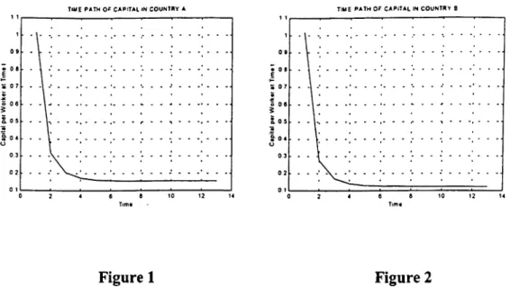
both on the transition path and at the steady state for two economies that are the same in every aspect except for population growth rates.

Figure 1 and Figure 2 show the time paths o f

k,

for two countries

A

and

В

with «.4 = 0.05 and «B= 0.2.

’ The results that are reported here are from a simulation with a = 0.4, p = 0.5, 6 = 0.7, // = 0.4, / =1,

k,=

1.0192, vv =0.8322.

TIME PATH OP CAPITAL IN COUNTRY A TIME PATH O f c a p i t a l IN COUNTRY B

Figure 1 Figure 2

The countries start with the same initial conditions in period 1. Figure 3 shows per capita capital stock in both countries starting from the second period onwards and until steady state is reached. It is clear from the figure that per capita capital stock in country

A

is greater than that in country

B,

at any point in time on the transition path as well as at the steady state.

TIME PATH OF CAPITAL IN BOTH COUNTRIES

Figure 3

The corresponding graphs for wages in countries

A

and

B

are given in Figures 4 and 5.

TIME PATH OF WAGE RATE IN COUNTRY A TIME PATH OF WAGE RATE IN COUNTRY B

Figure 4 Figure 5

Figure 6 excludes period 1, which is identical in both countries, and compare wage rates in the following periods. Again, we see that wages in the low population growth country

(A)

are always greater than those in the high population growth country at any time.

TIME PATH OF W AGES IN BOTH COUNTRIES

Figure 6

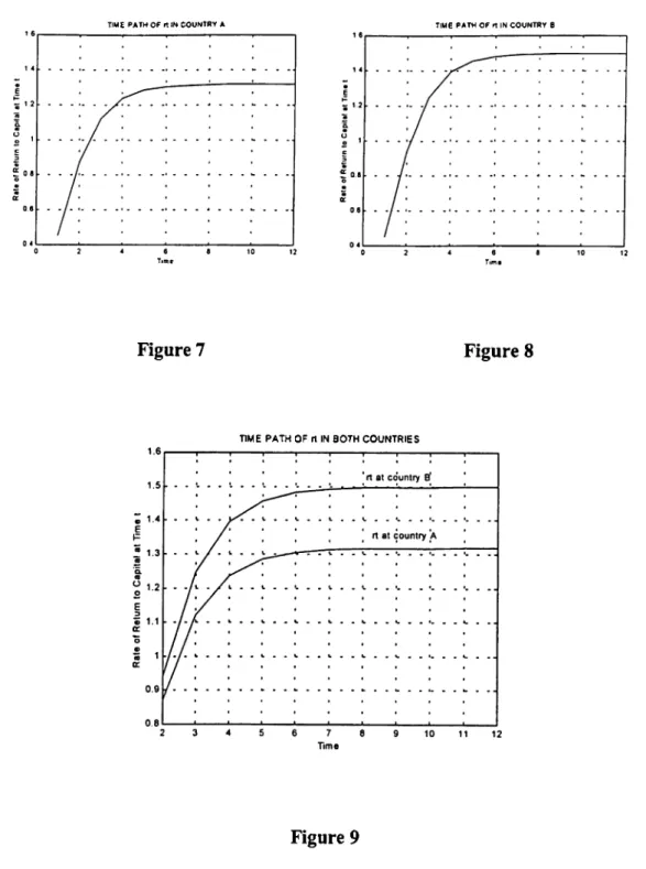
Figures 7, 8 and 9 contain the corresponding graphs for rental rate on capital

(r,)

in both countries. As expected, return on capital is lower on the relatively capital abundant country

(A)

in each period, as well as on the steady state.

TIME PATH OF f1 IN COUNTRY A TIME PATH OF ft IN COUNTRY B

Figure 7 Figure 8

TIME PATH OF r1 IN BOTH COUNTRIES

Figure 9

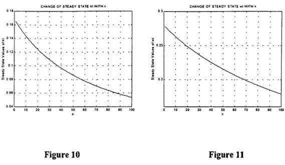
If we concentrate on the steady state values o f

k,

and

w,

corresponding to different values o f

n,

we reach the following result;

Steady state values of

kt

and w, are both decreasing functions o f

n,

for given values of constants a, p, 0, n, / and initial conditions ^, , vv. Figures 10 and 11 show this relationship between

kt

at the steady state and

n\

and W/ at the steady state and

n,

respectively.

CHANGE OF STEADY STATE M WITH n CHANGE OF STEADY STATE wt WITH n

Figure 10 Figure 11

The steady state values o f variables in both countries under autarky conditions are presented in Table 1.

Table 1

S te a d y State V a lue s

C o u n try A C ou ntry B

k

0 .1549

0.1244

w

0 .2710

0.2488

r

1.3175

1.4983

u

0 .11 78

0.1124

Our results show that, if the two countries are exactly the same initially, country

B

(i.e. the one with the higher

n)

ends up with a younger population

composition, lower

k,

and w, at the steady state when compared to country

A.

If full labor mobility between the two countries were allowed, one would expect a movement of labor from country

B

to country

A,

since the wage and utility differentials between these countries would provide an incentive for workers in

B

for migration to

A.

This migration and its consequences are discussed in Chapter 4.

CHAPTER 4

MIGRATION

In this chapter, we consider the results of allowing for labor mobility between these countries under two distinct scenarios. In the first scenario, the decision to migrate is based upon the difference between the lifetime utilities obtained in two countries and the migration is assumed to be from country

B

to country >4. In the second scenario, we allow for two-sided migration (i.e., either from 5 to ^ or from

A

to

B

in any given period) and the decision to migrate depends only on the wage difference. The process of migration, which is similar in both scenarios is as follows:

At time

t,

there are 2 kinds o f new-born workers in the source country: Workers that are able to migrate (which we call mobile workers) and workers that are unable migrate. A mobile worker bom at time

t

decides on whether to migrate or not by considering the current state o f the economy and the next two periods (in which he will live) under the assumption that none o f his fellow coimtrymen will choose to migrate to the other country during his lifetime. Immediately after birth, a mobile worker evaluates the variables o f concern (which are lifetime utilities in scenario 1 and wages in scenario 2) and compare the values that these variables

would attain in both countries, had there been no migration. We call these "variables under no migration"'® and denote them by adding the superscript

NM.

If the

To avoid a possible confusion, we would like to clarify one point. The phrase “variables under no migration” does not mean that these values are calculated by assuming that there is no migration at all, which would have made them equal to the autarky values. Rather, it suggests that these values are calculated by counterfactually assuming that there will be no migration in the next two periods. Since the mobile worker knows the current state of both economies and uses this information, the effects of actual labor movement up to this period are implicitly taken into account in his decision.

migration criteria is satisfied, the mobile workers will migrate from the source country to the receiving country and live both periods o f their lives there. The ratio o f mobile workers to the whole worker population in period

t

will be denoted by C/· h will be a function of in the first scenario and in the second scenario, as explained below.

Note that the change in number of workers due to migration results in a change in the values o f all variables in both countries, therefore the values that the workers use to make their decisions are not realized. Here, we relax the perfect foresight assumption by assuming that the value o f

Ct

is not common knowledge, so that a mobile worker is unaware of the other workers' decisions. Simply put, a worker looks at the future o f both countries and chooses one o f them to live in, by realistically assuming that his choice would have a negligible effect in this future, without knowing and taking into account how many others are making the same decision as him self

4.1.MIGRATION SCENARIO 1

The decision rule in this scenario is based on lifetime utilities o f workers in both coimtries that would have been realized if there had been no migration

^^BNM

j Ujjijifg Galor (1986) and Karayalcin (1994), where the workers from

country

B

migrate if

U f > U f

, we assume that there is a fixed cost associated with migrating permanently and the workers migrate only if the percentage increase in their utility is greater than a certain value. So, the decision rule for a mobile worker in country

B

is:

Migrate if

Tj ASM ^ Tj BNM

U.

BNM > T (4.1)

where t is an exogenously set constant.I I

The share o f mobile workers in the generation bom at time

t

in country

B

is given by

^ U BNM ^

ANM , T jB N M

+ f/

(4.2)

where z and

y

are positive constants.

After the migration, worker population in country

A

becomes

rjf

+

· rjf

) and the worker population in country

B

becomes (l - ^ , ) ·

r jf

, and the markets in both countries continue to work under autarky conditions.

Before moving on to the results o f this scenario, we should note how the values o f variables z and

y

characterize the process o f migration. If the workers in country

B

are very reluctant to migrate (i.e. z is very small and/or

y

is very big), the resulting migration will be very small when compared to the aggregate populations, therefore will not have a big impact. At the other extreme, if the workers in country

B

have a great tendency to migrate (with a very big value for z and/or y very small), a small difference in utilities may induce a large wave o f migrants, radically change

" T is taken as 0.01 in the simulation.

the number of workers in both countries and cause huge jum ps in the values o f variables, which is not a case that we are willing to consider. We stay away from these extremes and we z=l and y=1.5. The resulting steady state values in both coimtries are given in Table 2.

Table 2

M I G R A T I O N 1

A U T A R K Y

Steady State Values A B A B

k 0 . 1 24 6 0 . 1 2 4 6 0 . 1 5 4 9 0 . 1 2 4 4

w 0 .2 48 9 0 . 2 4 8 9 0 . 2 7 1 0 0 . 2 4 8 8

r 1.4969 1 .4 96 9 1 . 3 17 5 1 .4 98 2

u 0 . 1 12 4 0 . 1 1 2 4 0 . 1 1 7 8 0 . 1 1 2 4

Population Growth Rate 0 . 1 98 9 0 . 1 9 8 9

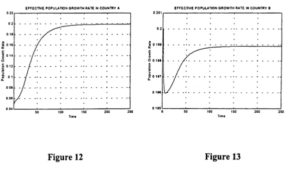
EFFECTIVE POPULATION GROWTH RATE IN COUNTRY A EFFECTIVE POPULATION GROWTH RATE IN COUNTRY B

Figure 12 Figure 13

One important result we obtain is that migration continues at the steady state with value o f ^ converging to a specific value (0.00090 in this simulation) which equalizes population growth rates in both countries. This result is different from the

results of the Galor (1986), who, in a different setting, modeled a migration scheme which results in whole population of a country migrating to another country. Time paths o f population growth rates in both countries are given in Figures 12 and 13.

We may interpret the resulting steady state as the case o f two countries under autarky conditions, each with a population growth rate o f 0.1989. This is very close to ns = 0.2, as expected, since country

B's

population grows so large when compared to country

A

that only a small portion o f its increment is enough to equalize the population growth rates. Still, the effective population growth rate (which is the after migration population growth rate) in country

B

is less than the autarky case and the residents o f country

B

are slightly better off’^ with higher utility, wage rate and per capita capital stock at each period. However, the migrants in the early periods benefit a great deal.

A COMPARISON OF UTILITIES OF MIGRANTS AND NONMIGRANTS

Figure 14

In this simulation, the percentage increase in utility of a resident o f country B is on the order of

0

.

01

%.

Figure 14 shows the graphs o f lifetime utility o f a migrant to country

A

and the lifetime utility of a worker staying at country

B.

While these converge to the same level at the steady state, the benefit o f the migrants in early periods are clearly visible in the figure.

Obviously, residents of country

A

experience an effective population growth rate that is much higher than nA = 0.05 and are made worse off in each period as well as in steady state as a consequence o f facing smaller

kt, w,

and

Ui

values.

4.2.MIGRATION SCENARIO 2

In this scenario, we allow for bilateral migration with decision criteria being the "wages under no migration" in both countries. So, the decision rule is:

( I )If >

w¡

BUM Migration is from

B io A

C = ^

( II )if > w;

Am

Migration is from

A to B

r am

_{-w ,}

ANM Y

(4.3)

The results o f this scenario is given in Table 3, with which is the rate o f migration from

A io B

being 0 at all times and

if,

the rate of migration from

B to A

converging to 0.00422 at the steady state.

Table 3

M I G R A T I O N 2

A U T A R K Y

Steady State Values B B

0.1252 0 .1 25 2 0 . 1 5 4 9 0 . 1 2 4 4

w 0 . 24 94 0 . 2 4 9 4 0 . 2 7 1 0 0 . 2 4 8 8

1.4921 1.4921 1 . 3 1 7 5 1 .4982

0 .1 12 6 0 . 1 1 26 0 . 1 1 7 8 0 . 1 1 2 4

Population Growth Rate 0 .1949 0 . 1 9 4 9

First thing to note is that the qualitative results are same in both migration scenarios. This is due to the fact that we restrict the migration process to be a smooth one, i.e. one that does not cause large jumps in population compositions. As a result, the gap between the wages in both countries decreases gradually and finally disappears. Note that.

which is the case at the steady state. Therefore, wages in country

B

can never pass the wages in country

A,

causing the migration to be one sided in practice, even though migration in the opposite direction is theoretically possible.

Making a comparison between two migration scenarios is not meaningful, since the relative positions of the countries in steady state under these two different scenarios depend on the initial states. The important point here is that comparing either migration scenario with autarky cases (and the trade scenarios as we will explain in the next chapter) gives the same results.

CHAPTER 5

TRADE

In this chapter, we examine the results of trade between these two countries under the assumption that both countries are equal in size initially. A second trade scenario where country A is taken to be a large country (in the same sense as used in the trade literature) and country

B

is taken to be a small country is discussed in Appendix B.

A natural result of free trade will be the equalization o f prices in both countries in each period so

V/ (5.2)

In the present version o f our model, we do not allow for foreign direct investment and factor movements between countries. However, given that good 1 is used for both consumption and investment purposes, capital stock at time

t

comes from good 1 produced at time

t-1.

Therefore, while installed capital itself is immobile between countries, some of good 1 traded in the previous period may be used as

capital in the current period.

The capital abundant country (country

A)

specializes in the production o f the relatively more capital intensive good (good 2) and exports it, while the labor

abundant country (country

B)

specializes in the production o f and exports the relatively more labor intensive good (good 1).

Instead of market clearing conditions in each country (as in the autarky case), we require that world-wide demand to both goods is equal to the world-wide supply, meaning that the amount of good 2 (good 1) that country

A

exports (imports) is equal to the amount o f good 2 (good 1) that country

B

imports (exports). This requires that the following equations hold.

x^,

+ k

:^ -

-

Tif ■

c - 7,1. · C =

rif ■

C + ·

c l ,

+

K l , - X l - K f

(5.3)

\ r A A f-^A A ^ A b . B y-B

^ 2 / V / ’ ^2jy/ V i-1 ' ^ 2 o i “ V / *^ 2> 'r V /-1 ' ^ 2 o t ^ 2 / (5.4)

enabling us to determine the world price once

k f

and

k f

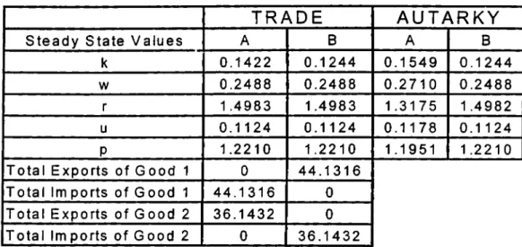
are known. The resulting steady state values for both countries are reported in Table 4.

Table 4

T R A D E

A U T A R K Y

s t e a d y State Values A B A B k 0 .1 42 2 0 . 12 44 0 . 1 5 4 9 0 . 1 2 4 4 w 0 .2 48 8 0 . 2 4 88 0 . 2 7 1 0 0 . 2 4 8 8 r 1.4983 1.4983 1 .3175 1 .4982 u 0 . 11 24 0 . 1 1 24 0 . 1 1 7 8 0.1 124 P 1.2210 1.2210 1.1951 1 .2210

Total Exports of Good 1 0 4 4 . 1 3 1 6

Total Imports o f G o o d 1 4 4 . 1 3 1 6 0

Total Exports o f G o o d 2 3 6 .1 4 32 0

Total Im ports of Good 2 0 3 6 . 1 4 3 2

We see that all o f the variables in country

B

converge to their steady-state autarky values. Wages, rental rates, prices and utility in country

A

have the same steady state values as country

B.

Capital per worker in

A

is higher than that o f

B,

but it is smaller than the value it would have attained under autarky. The results indicate that, in the long run, country

B

behaves as if it were a large country, while country

A

becomes and acts like a small country. This is due to the large population difference that occurs between

A

and

B

over time. Resulting from the high population growth rate in country

B,

this population difference between the two countries grows bigger as time passes. Although country

A

is advantageous in terms o f per capita variables, its aggregate production and demand remains very small when compared to aggregate production and demand o f country

B.

After a certain time, country

A ’s

contribution to the world economy becomes negligible, so the results obtained by solving the model for the world become nearly the same as the results obtained by solving only for coimtry

B.

This means that although we did not require any country to be large in the beginning, the difference in demographics cause country

B

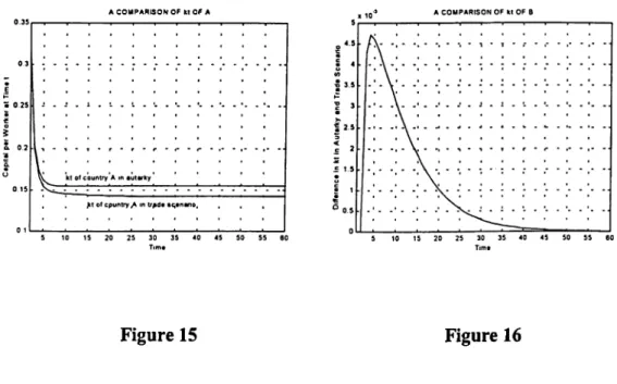
to practically become the large country.

A COMPARISON OP M OP A

Figure 15 Figure 16

Figure 15 contains a graph comparing the time path o f

k f

under autarky and under the trade scenario. Comparison of time paths o f

k f

in these two cases is given

in Figure 16 which plots the difference between

k f

imder the trade scenario and

k f

under autarky

{kf^'‘“‘‘ - k f

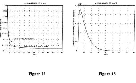
^“'"'^') better inspection. Similar plots comparing lifetime utilities in both countries are given in Figures 17 and 18.

A COMPARISON OF Ut of A A COMPARISON OF Ut of B

Figure 17 Figure 18

In the initial periods, where the effect o f the differences in population growth rates are relatively small, country

B

actually benefits from trade, as in the previous scenario. Trading with country

A,

which has higher

kt

and tower

p,,

results in lower prices and higher capital per worker for country

B

during the initial stages o f transition. However, the effect of the difference between population growth rates induces country

B

to start behaving as a large country after some time and therefore diminishes the benefits of trade for that country. The effect of population growth differences grow stronger as time passes, totally dominating the process eventually and causing the values o f all variables in country

B

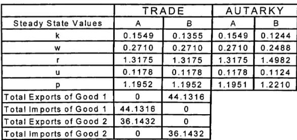
to converge to their autarky values.

When we compare the current trade scenario with the one presented in Appendix B (i.e., the one where country

A

is the large country), we see that the one in Appendix B is more realistic in two main aspects. First o f all, the scenario presented here results in a net welfare loss for country

A,

implying that this country will have no intention to take part in such a trade in the first place. One justification o f such a scenario may be a case where country

A

faces a choice between trading with country

B

and accepting migrants from country

B.

I f country

A

has no other means o f avoiding full labor mobility between these countries (as in the European Union), it may be willing to bear the burden of such a trade if the consequences o f migration are more severe for it.

However, when we compare the case o f migration with that o f trade, we see that the argument in favor o f the trade scenario can not be Justified immediately. Figure 19 clearly shows that the residents o f country

A

are also better off under migration scenario 1 on the transition path as well as at the steady state. However, the difference in steady state values is too small to provide a basis for a clear-cut decision, so that we can consider them as equal and this may lead to a justification o f the current trade scenario. The fact is that most o f the social factors that are non­ existent in our model (such as cultural differences, increasing crime rates, etc.) do not favor accepting migrants. This may motivate country

A

to engage in trade with coimtry

B

to avoid migrants, since the economic outcome for country

A

would be the same in the long run.

Figure 19

Of course, if country

A

is actually a large country when compared to country

B,

the trade would take place and would not cause a welfare loss for either country (see Appendix B). In such a case, the equalization o f prices would eliminate the motive for migration, with country

B

moving up to the level o f country

A

rather than country

A

moving down to the level o f country

B,

which would happen in the case o f migration.

Trade scenario in Appendix B has another advantage over the one in this chapter in terms o f its relevance to real life examples o f the issue under consideration. When we consider such examples (such as EU vs. Turkey, USA vs. Mexico), we see that country that we model as

A

has a much bigger aggregate economy than that of country

B.

Therefore taking country .,4 as a large country becomes a much more realistic assumption.

these modifications have absolutely no effect in the autarky case, they may turn out to be important in a trade scenario, where the relative sizes o f populations affect the outcome in a particular period. However, such an effect does not exist in the long run. We observe that the steady state values o f the per capita variables are completely unaffected and turn out be equal to the values reported in Table 5.

Clearly, as time passes, the effect caused by differences in population growth rates dominate the effect of initial population differences. As a result, the initial population compositions may weaken (or strengthen if initial population o f country

B

is bigger) the effect o f n ’s, alter the time path and change the length o f the transition period until the steady state is reached, but have no effect on the level o f steady state values of variables.

CHAPTER 6

CONCLUSION

In this thesis, we examined the effects o f differing population growth rates and resulting age composition differences across countries on the m igration and trade patterns. We considered two countries that have the same initial conditions and exactly the same properties except for the population growth rates, and compared the time paths and steady state values of variables like capital per worker, wage rate, rate o f return to capital and lifetime utility. We showed that a difference in population growth rates is enough to provide incentives for flow o f labor and/or commodities across countries. We modeled international labor migration and examined its effects on both the source and the host country. International trade is also modeled under two different assumptions (with and without allowing for one o f the countries to be large) and the consequences o f trade are compared with those o f migration.

Before moving on to our main results regarding migration and the comparison o f trade and migration scenarios, we briefly comment on the autarky cases. Since the countries start with exactly the same initial conditions, the values o f variables for both of them are the same at the end o f the first period. At the beginning o f the second period, while they continue to have the same total capital, population (and hence, labor supply) in country

B

becomes higher than country

A,

causing capital per worker in country

A

to rise above country

B.

As a result, country

B

becomes the labor abundant country with a comparative advantage in producing the relatively more labor intensive good (good 1). Country

A,

on the other hand, turns

into the capital abundant country with a comparative advantage in producing the relatively more capital intensive good (good 2), as reflected by the difference

between the relative prices in both countries.'^

The simulation results suggest that the wage rate and capital per worker are lower in country

B

(where labor is abundant), while the return on capital is lower in country

A

(where capital is abundant). Moreover, the representative consumer in country

A

always attains a higher level o f lifetime utility than his counterpart in country

B.

The first result that we obtain from migration scenarios is that the two scenarios are the same in practice. The difference between these scenarios is that migration scenario 1 only allows for one-sided migration (from

B

to

A)

whereas two- sided migration is theoretically possible in migration scenario 2. However, the two scenarios become essentially the same if no incentive to migrate from

B Xo A

arises (i.e., if the wage rate in

B

never exceeds that in

A),

which is exactly what happens in the present simulation. This is due to the restriction that the migration scheme we consider be a smooth one so as not to observe discontinuity in the values o f variables, which is a fairly realistic restriction. This migration scheme does not lead to any irregularities such as a large amount o f people migrating in one period followed by no migration in the next period, as instantaneous jumps are ruled out. Given that the wages in

A

are initially higher than those in

B,

if the wages in

B

were ever to exceed

A,

they should first become equal (or at least sufficiently close). At first, the large difference between

wf

and wf (in favor of

A)

provides a big

A similar argument applies to all periods, meaning that country A should always have comparative advantage in producing more capital intensive good, which is indeed the result of the simulation.

incentive for migration from

B to A.

As the system moves closer to steady state, the difference between

wf

and

wf

gradually decreases, reducing the incentive to migrate. At the steady state when

wf

and wf become virtually equal (note that there is still incentive to migrate from

B to A

since ), the amount o f migration is not enough to push wa lower than wb

.

Therefore, no migration from

A

to

B

ever occurs, reducing the effects observed under migration scenario 2 to those observed imder migration scenario 1.

Another important result obtained from the migration scenarios is the convergence o f the rate o f migrating workers in country 5 to a value that equalizes

population growth rates in both countries at the steady state. This result is significantly different than Galor (1986), where the migration does not affect wages causing the incentive to migrate to persist on the adjustment path. This, in turn, results in the migration o f the whole population of one country to the other. In our model, migration serves to equalize relative prices and factor prices. The welfare effects are in line with Galor (1986) and Karayal9in (1999) in that the host country

gets worse-off while the source country remains at least as well-off (becomes slightly better-off to be exact).

One feature of the adjustment path in migration scenarios is that the length o f the transition period is much longer than that o f the autarky cases. This causes the resulting common population growth rate (0.1989 in scenario 1 and 0.1949 in scenario 2) to be very close to hb

,

which is 0.2. Since the ratio o f the youngs bom in country

B

to those bom in country

A

grows larger and larger over time, the length o f the path to steady state makes the movement o f only a small portion o f youngs in

B

sufficient to equalize population growth rates across countries. As a result, citizens of

A

incur a great welfare loss due to the migration while the welfare o f citizens o f

B

at the steady state is almost the same under autarky and migration. This, however does not suggest that the migrants’ decisions to migrate are without justification. The time paths of the welfare o f the migrants and the non-migrants show that the migrants benefit greatly from migrating, especially in the initial periods.

We also see that we were not mistaken to assume that individuals decide whether to migrate or not by comparing the “imder no migration” values o f utilities (or wages in migration scenario 2) and ignore the fact that these values would not be

realized after migration. While the individuals do ignore some effects by doing so and the improvements in their welfare turn out to be smaller than they anticipated, they are stilt better-off as compared to the non-migrants, justifying that they were right to decide in favor o f migrating in the first place.

Our trade scenarios exhibit the usual characteristics o f Heckscher-Ohlin type models with each country specializing in and exporting the good in the production of which it has a comparative advantage and importing the other good. Before moving on to the more interesting case o f the comparison o f results o f trade scenarios with those of migration scenarios, we would like to comment on a few things.

Clearly, results of trade scenario in chapter 5 imply a Pareto deterioration for country

A

and are contrary to a common result in the trade literature which suggests that none of the parties involved in international trade should face welfare losses. This result might have changed if we had considered compensation schemes or transfer payments between countries. Some studies using OLG models, such as

Kemp and Wong (1995) and Roy and Rassouli (1991), argue that the absence o f these mechanisms may result in free trade being inferior to autarky. Bohm and Keiding (1985) also present an OLG model with inflation where all agents o f one country are made worse off under free trade. However, the real reason behind the welfare loss in our trade scenario is that country

A

is essentially forced to act as a small country in the long run and take the prices realized in country

B

because o f the significantly faster population growth in this country. This increases the relative price in country A while the wages fail to compensate the effect o f this increase. This result is in line with Galor (1988a, 1988b), who suggest that free trade may cause a Pareto deterioration for a small country in the absence o f international transactions in financial assets.

Since migration is also Pareto inferior to autarky, the best solution for country

A

seems to close its borders to both labor and good movements if it is not a large country. A possible reason for not doing so may be country

A ’s

inability to prevent legal (which would probably be the case should Turkey be accepted as a full member by the EU) or illegal (which is the case between Mexico and the U.S.) migration o f labor. What country

A

may do instead may be to try to eliminate motives for migration by engaging in trade with country

B.

(We would like to remind that one o f the arguments raised in the U.S. in defense of NAFTA was that it would slow down labor migration from Mexico to the U.S. by increasing wages in Mexico.)

At a first glance, engaging in trade to avoid migration does not seem to be a rational choice for country .,4, if it does not have the power o f imposing its own prices

as a large country, as in the scenario in chapter 5. While migration, which pushes country

A

close to the welfare level o f country

B

under autarky and causes a net