Gravity anomaly separation using 2 - D wavelet approach and average depth calculation

GRAVITY ANOMALY SEPARATION USING 2-D

WAVELET APPROACH AND AVERAGE DEPTH

CALCULATION

A. Muhittin Albora

Istanbul University, G eophysics D epartm ent

Osman N. Uçan

Istanbul University, Electric and Electronics D epartm ent

A B S TR A C T: In this paper, 2-D Multi-Resolution Analysis (MRA) is used to per­ form Discrete-Parameter Wavelet Transform (DPWT) and applied to gravity anom­ aly separation problem. The advantages of this method are that it introduces little dis­ tortion to the shape of the original image and that it is not effected significantly by fac­ tors such as the overlap power spectra of regional and residual fields. The pro­ p o s ed method is tested using a synthetic example and satisfactory results have been found. Then average depth of the buried objects have been estimated by power spectrum analysis.

Keywords: Wavelet, Gravity anomaly, Power spectrum analysis.

ÖZET: Bu makalede, gravite anomalilerinin ayrım problemi için Discrete- Parameter Wavelet Transform (DPWT) 2-B Multi-Resolution Analizi (MRA) kullanıldı. Yüzeye yakın kürelerin ortalama derinliklerini bulmak için güç spekturum analizi kullanıldı. Yöntemin geçerliliğini test etmek için sentetik yapılar kullandık ve memnun edici neticeler bulduk. Gömülü cisimlerin ortalama derinliklerinin hesaplanması için güç spektumu kullanıldı.

Geophysical maps usually contain a number of features (anomalies, structures, etc.) which are superposed on each other. For instance, a magnetic map may be composed of regional, local, and micro-anomalies. The aim of an interpretation of such maps is to extract as much useful information as possible from the data. Since one type of anomaly often masks another, the need arises to separate the various features from each other.

One of the main purposes of geophysical mapping is the identification of units that can be related to the unknown geology. On a regional scale, aeromagnetic and gravity maps are most useful tools presently available, although other techniques such as conductivity mapping (Palacky, 1986) or remote sensing (Watson 1985) are very helpful in locating lithologic boundaries. The interpretation which makes extensive use of enhanced maps of gravity data often involves initial steps to eliminate or attenuate unwanted field components in order to isolate the desired anomaly (e.g., residual-regional separations). These initial filtering operations include the radial weights methods (Griffin, 1989), least squares minimisation (Abdelrahman et al., 1991), the Fast Fourier Transform methods (Bhattacharyya, 1976) and recursion filters (Vaclac et’al, 1992) and rational approximation techniques (Agarwal and Lal, 1971). Gravity anomaly separation can be effected by such wavelength filtering when gravity response from the geologic feature of interest (the signal) dominates one region (or spectral band) of the observed gravity field’s power spectrum. R.S. Pawlowski et’al (1990) has investigated a gravity anomaly separation method based on frequency-domain Wiener filtering. S. Hsu et’al (1996) has presented a method for geological boundaries from potential-field anomalies.

In this paper, 2-D Wavelet is applied to gravity anomaly map on real time. This modern and real time signal processing approach is tested using synthetic examples and perfect results have been found. So we can offer 2-D wavelet as an alternative to classical gravity anomaly separation methods.

This paper is organised as follows. In Section II, Problem Statement at Gravity Anomaly Map is presented. In Section III, 2-D Wavelet Transforms and M ulti­ Resolution Analysis (MRA) is explained. In Section IV, Wavelet Application on Gravity Anomaly Map is tested using a synthetic examples and satisfactory results have been observed. In the last Section, average depth of the buried objects have been estimated using power spectral approach.

H PROBLEM ST ATEMENT AT GRAVITYANOMAL Y MAP

Traditionally, magnetic and gravity maps are subjected to operations approximating certain functions such as second derivative and downward continuation (Pick et'al, 1973). Gravity data observed in geophysical surveys are the sum of gravity fields produced by all underground sources. The targets for specific surveys are often small-scale structures buried at shallow depths, and these targets are embedded in a regional field that arises from residual sources that are usually larger or deeper than

the targets or are located farther away. Correct estimation and removal of the regional field from initial field observations yields the residual field produced by the target sources. Interpretation and numerical modelling are carried out on the residual field data, and the reliability of the interpretation depends to a great extent upon the success of the regional-residual separation.

In literature some classical methods are proposed for the seperation of gravity maps. The simplest is the graphical method in which a regional trend is drawn manually for profile data. Determination of the trend is based upon interpreter’s understanding understanding of the geology and related field distribution This is a subjective approach and also becomes increasingly difficult with large 2-D data sets. In the s econd approach, the regional field is estimated by least-squares fitting a low-order of the observed field (Abdelrahman et al., 1991) . This reduces subjectivity, but still needs to specify the order of the polynomial and to select the data points to be fit. The third approach applies a digital filters such as Wiener filtering to the observed (R.S. Pawlowski et’al, 1990).

In this study, one of the very update 2-D image processing technique, Wa v e l e t approach is applied to gravity anomaly map and satisfactory results are observed. m . 2-D WAVELET TRANSFORMS AND MULTI-RESOLUTION ANALYSIS The wavelets, first mentioned by Haar in 1909, had compact support which means it vanishes outside of the finite interval, but Haar wavelets are not continuously differentiable. Later wavelets are with an effective algorithm for numerical image processing by an earlier discovered function that can vary in scale and can conserve e nergy when com puting the functional energ y. In betw een 1960 and 1980, mathematicians such as Grossman and Morlet (1985) defined wavelets in the context of quantum physics. Stephane M allat (1989) gave a lift to digital signal processing by discovering pyramidal algorithms, and orthonormal wavelet bases. Later Daubechies (1989, 1990) used M allat’s work to construct a set of wavelet orthonormal basis functions that are the cornerstone of wavelet applications today. A- Wavelet Transforms:

The class of functions that present the wavelet transform are those that are square integrable on the real line. This class is denoted as L 2 (R).

The set of functions that are generated in the wavelet analysis are obtained by dilating (scaling) and translating (time shifting) a single prototype function, which is called the mother wavelet. The wavelet function \j/ ( x ) e L 2 ( R ) has two characteristic parameters, called dilation (a) and translation (b), which vary continuously. A set of wavelet basis function y/ b ( x ) may be given as

Here, the translation parameter, "b", controls the position of the wavelet in time. The "narrow" wavelet can access high frequency information, while the more dilated wavelet can access low frequency information. This means that the parameter "a" varies for different frequencies. The continuous wavelet transform is defined by

+00

wa,b( f ) = < f ’¥<,*>= \ f { x ) y / atb{ x) dx.

(3)

—oo

The wavelet coefficients are given as the inner product of the function being transformed with each basis function.

Daubechies (1990) invented one of the most elegant families of wavelets. They are called compactly supported orthonormal wavelets, which are used in discrete wavelet transform (DWT). In this approach, the scaling function is used to compute the (if. The scaling function $0) and the corresponding wavelet ((c (x) are defined by

(/>{x) = Ÿ Jck </>{2x-k)

(4>

k = 0

N - 1

0 ( 2 x + k - N + 1)

<5>

k=0

where N is an even number of wavelet coefficients, c . . k= 0 )o N- ) . The discrete presentation of an orthonormal compactly supported wavelet basis of

L \ R )

V j , k

(*) =

(6>

and, the discrete-parameter wavelet transform (DPWT) is defined as

DPW T(f) =< f,v|/j k >= Jf(x)a0_ j /2 \|/(a0_ jx - k b 0)dx

(7)

The dilations and translations are chosen based on power of two, so called dyadic scales and positions, which make the analysis efficient and accurate. In this case, the frequency axis is partitioned into bands by using the power of two for the scale parameter "a". Considering samples at the dyadic values, one may get bQ = 1 and a 0 = 2 , and then the discrete wavelet transform becomes

1-W . , ^ .

Here, ¥ j , k ( * ) is defined as

¥ j , k (* ) = 2_7/2 y ( X j x - k )>

M e Z

(9)

B- Multi-resolution Analysis (MRA)

Mallat (1989) introduced an efficient algorithm to perform the DPWT known as the Multi-resolution Analysis (MRA). It is well known in the signal processing area as the two-channel sub-band coder. The MRA of .¿2 ( * ) consists of successive approx­ imations of the space y 0.. j0- c ^ \ There exist a scaling function ^ ( (..) e y such

that J 0

(/>Jtk(x) = 2~j n ^(2~j x - k ) ;

j , k e Z (

)

For the scaling function G

V0 d Vx

{hk

t ( x ) = 2 '£ l hk </>{2x-k).

(

11

)

k

This equation is known as two-scale difference equation. Furthermore, let us define j y as a complementary space of y . ( . y . , such that y . = y . 0 fy , and

+ 0 0

© Wj = L \ R ) . Since the (() . is a wavelet and it is also an element of V0 , a sequence ( g ( ■ exists such that

V ' ( x ) = 2 ' £ i g k 0 ( 2 x - k )

k

It is concluded that the multiscale representation of a signal f(x ) may be achieved in different scales of the frequency domain by means of an orthogonal family of functions ^ (

x

f

Pvf i (x) = Y . cj,k<l>j,k (x )

(

)

k

Here, C. k = < f . ( j . ( X( > • Similarly, the projection of the function f(x ) on the subspace is also defined by

pj

1( x ) = Y é d i * y ' J x )

(i4)

where d j k =< f , ^(c j k ( x ( >. Because of V ■ = V _x © W -_x , the original function e V can be rewritten as

J - 1

f { x ) = ^ cJJk ÿ j t (x) + £ Y s d j,k ¥j,k (*)

J > Jo

(

)

The coefficients C j _ j and d j ^j are given by ( 16) i and dj,k — ^ &j~2k CJ-k ' (17) y

The m ultiresolution representation is linked to Finite Impulse Response (FIR) filters. The scaling function j and the wavelet Ware obtained using the filter theory and consequently also the coefficients are defined by these last two equations. If at x=t/2, j | j (jj) } is considered and

As ^ ( 0) ^

0

H (a> )G *(a> ) + H (co + 7t) G * (co + n ) = 0 . Here, H (o) and G)oo) are quadrature mirror filters for MRA solution.

G {co) - - e x p ( - j a ) ) H * ( a > + n ) (19) Substituting #(0)=1 and H(n)=0, it yields G(0)=0 and G(n) =1, respectively. This means that Q)oo) is a high pass filter. As a result, the MRA is a kind of two-channel sub-band coder used in the high-pass and low-pass filters, from which the

original signal can be reconstructed.

Since a major potential application of wavelets is in image processing, 2-D wavelet transform is a necessity. The subject, however, is still in an evolving stage and this section will discuss only the extention of 1-D wavelets to the 2-D case. The idea is to first form a 1-D sequence from the 2-D image row sequences, do a 1-D MRA, restore the MRA outputs to a 2-D format and repeat another MRA to the 1-D column sequences. The two steps of restoring to a 2-D sequence and forming a 1-D column sequence can be combined efficiently by appropriately selecting the proper points directly from the 1-D MRA outputs. As seen in Figure 1, after the 1 -D row MRA, each lowpass and highpass output goes through a 2-D restoration and 1-D column formation process and then move on to another MRA. Let t, and t2 , be the 2-D coordinates and L=lowpass, H=highpass. Then the 2-D separable scaling function is

(18)

G restoration of 2-D and form H H restoration of 2-D and form G H

s3

s4

* <w( t l . t 2) = * ( t l ) t ( t 2) , LL

original signal can be reconstructed. Then 2-D separable wavelets are V <V(h>t 2 ) = ^ ( t\ ) v ( h ) > L H

V (V( h ’t2) = W(t\)<l>(t2) ’ HL

V (4) ( t l , t 2) = i ( t l M t 2) , H H

with the corresponding wavelet coefficients s2, s3 and s4. It is easy to verify that the j'' nn are orthonormal wavelets, i.e.,

\ \ v (i)( t v t2) d t x dt2

=0

The scheme of separable 2-D processing, while simple and uses available 1-D filters, has disadvantages when compared to a genuine, 2-D MRA with non-separable filters. The latter possesses more freedom in design, can provide a better frequency and even linear phase response, and have non-rectangular sampling.

IV. WAVELETAPPLICATION ON GRAVITYANOMAL Y MAP

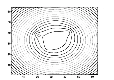
In this section, we have tested our proposed approach to some synthetic data and perfect results have been obtained. All the units used in examples are normalized values. In the first example (Table I) four spherical structures are used. For increas­ ing regional effects on Bouguer anomaly map (Figure 2), the big sphere with the biggest radius is replaced deeper than the others. Also to increase the residual effect, the other spheres are closer to the ground. At wavelet output, the residual map is extracted satisfactory as shown in Figure 3.

Parameters sphere 1 sphere 2 sphere 3 sphere 4

Coordinate (x,y) (32,32) (44,42) (24,40) (30,26)

h 100 5 4 4

r 30 4 4 3

p (gr / cm3) 1.8 1.2 1 1.3

Table 1 : Parameters of Bouguer anomaly map of an Example.

Figure 2. Bouguer Anomaly of four spheres with parameters as in Table I.

Figure 3. 2-D Wavelet output of the Bouguer Anomaly given in Figure 2 (Level 2, Daubechies 2).

V. DEPTH ESTIMATION USING POWER SPECTRAL PROPERTIES

One of the main researches on gravity anomaly maps is to estimate the average depth of the buried objects resulting the anomaly. In interpretation of gravity anomalies by means of local power spectra, there are three main parameters to be considered. These are, depth , thickness and density of the disturbing bodies. In direct interpretation, the information such as the maximum depth at which the body could lie and depth estimates of the centre of the body are obtained directly from the gravity anomaly map. It is clear that infinite number of different configurations can result in identical gravity anomalies at the surface and in general, gravity modelling is ambigous. In indirect interpretation the simulation of the causative body of the gravity anomaly is computed by simulation. The variables defining the shape, location, density etc. of the body are altered until the computed anomaly closely matches the observed anomaly. As it is well known potential fields obey Laplace's equation which allows for the manipulation of the gravity in the wavenumber domain. Many scientists have used the calculation of the power spectrum from the Fourier coefficients to obtain the average depth to the distirbing surface or eqivalently the average depth to the top of the disturbing body (A. Spector and Grant 1970).

It is necessary to define the power spectrum of a gravity anomaly in relation to the average depth of the disturbing interface. It is also important to point out that the final equations are dependent on the definition of the wavenumber in the Fourier transform. For an anomaly with n data points the solution of Laplace equation in 2D is,

n - 1

i27tkx:

+ ')-\C7

g ( x : , z ) = I A k e

J e -

(26)

j = 0

where wavenumber k is defined as (; = ) / ^ 00o ( are therefore the amplitude

coefficients of the spectrum, ^

n - 1

— i2itkx :

+

-W

A k = I g ( x | , z ) e

J e - 27Tkz.

(27)

j = o J

for z=0, equation (27) can be written as,

n - 1

- i2rckx :

(A k ) 0 = 2 g ( x : ,0 ) e

J .

(28)

j = 0

J

Then equation (27) can be rewritten in terms of (28) as,

A k = ( A k ) 0 e±27lkZ-

(29>

Then the power spectrum Pk is defined as,

Taking logarithm of both sides,

l°Se Pt = lo g e(-Pt )o± 4 ? r k z (31)

we can plot wavenumber, k, against

l°Se pk

The interpretation of the 1 o g e against wavenumber k requires the best fit line through the lowest wavenumbers of the spectrum. The wavenumbers included in this procedure are those smaller than the wavenumber where a change in gradient is observed. Then average depth can be estimated from plotting of Equation (31) as,

h = i ^ k (32)

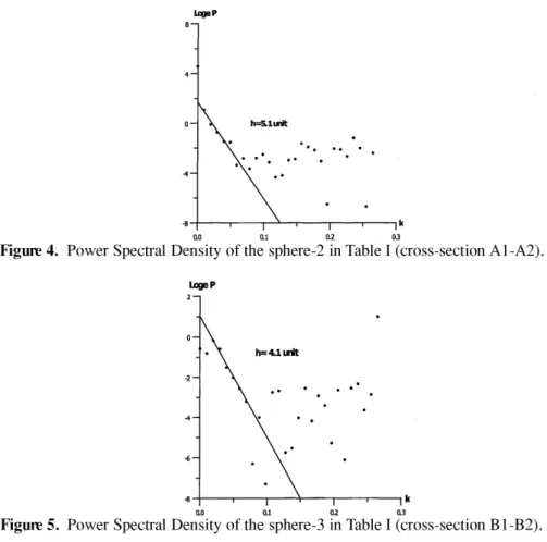
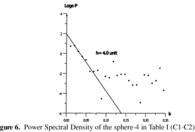
where h is the average depth, AP and A k are derivative of P and k respectively. In this paper, we have estimated the spheres depths using power spectral approach with high accuracy as shown in Figures (4-6).

LogeP

Figure 4. Power Spectral Density of the sphere-2 in Table I (cross-section A1-A2).

LogeP

LogeP

Figure 6. Power Spectral Density of the sphere-4 in Table I (C1-C2). VI. CONCLUSION

In this paper, wavelet approach has been applied to gravity anomaly separation problem. The proposed method is tested using a synthetic example and satisfactory results have been found. Then average depth of the buried objects have been estimated by power spectrum analysis.

ACKNOWLEDGEMENT

This project is supported by Research Fund of University of Istanbul. Project No.1409/05052000.

REFERENCES

ABDELRAHMAN, E.M., A.I., BAYOUMI, H.M. EL-ARABY. (1991), "A l e ast­ squares minimization approach to invert gravity data”, Geophysics, 56, 115-118

AGARWAL, B.N.P., AND LAL, L.T. (1971), "Application of rational approximation in the ca lc u latio n of the second deriv ativ e of the g ravity field", Geophysics, 36, 571-581.

A. SPECTOR AND F. S. GRANTI. (1970), "Statistical models for interpreting aeromagnetic data", Geophysics, 35, 293-302.

BHATTACHARRYYA, B.K., AND NAVOLIO,M.E.(1976), "A Fast Fourier Transform method for rapid computation of gravity and magnetic anomalies due to arbitrary bodies",Geophysics, Prosp., 20, 633-649.

CHAN Y.T. (1996), "Wavelet Basics",Kluwer Academic Publishers, USA.

DAUBECHIES,I. (1990), "The Wavelet Transform, Time-Frequency Localization and Signal Analysis", IEEE Trans. On Information Theory, 36.

E. ISING, (1925), "Zeitschrift Physik", 31, 253.

GABOR, D. (1946), "Theory of Communications", J.IEEE, 93, 3, 429.

GRIFFIN, W.P. (1989), "Residual gravity in theory and practice", Geophysics, 14, 39-56.

GROSSMAN,A.,MORLET,J. (1985), " Mathematics and Physics", 2, L. Streit, Ed., World Scientific Publishing, Singapore.

MALLAT, S. (1989), "A Theory for Multiresolution Signal Decomposition the Wavelet Representation", IEEE Trans. Pattern Anal. And Machine Intelligence, 31, 679-693.

PALACKY, G.J.(1986), "Geological background to resistivity mapping, in, Ed., Palacky, G.J., Airborne resistivity mapping",G.S.C. Paper 86-22,19-27. PICK, M., PICHA,J., AND VYSKOCIL, V. (1973), "Theory of Earth’s gravity

field", Academia

R.S.PAWLOWSKI, AND R.O. HANSEN, (1990), "Gravity anomaly separatiin by Wiener filtering", Geophysics , 55, 539-548.

RICHARD C. DOBES, ANIL JAIN, (1989), "Random field models in image analysis", Journal of Applied Statistics, 16, 131-162.

SHU-KUN HSU, JEAN-CLAUDE S., AND CHUEN-TIEN S. (1996), "High­ resolution detection of geological boundaries from potential-field anom­ alies; An enhanced analytical signal technique", Geophysics, 61, 373-386. VACLAC B., JAN H., AND KARELS. (1992), "Linear filters for solving the direct

problem of potential fields", Geophysics, 57, 1348-1351.

WATSON, K., (1985), "Remote sensing: A geophysical perspective",Geophysics. 55, 843-850.

YAOGUO LI., AND DOUGLES W. O. (1998), "Separation of regional and residual magnetic field data",Geophysics, 63, 431-439.