Consequences of COVID-19 on the social isolation of the Chinese
economy: accounting for the role of reduction in carbon emissions
Daniel Balsalobre-Lorente1 &Oana M. Driha2&Festus Victor Bekun3,4&Avik Sinha5&Festus Fatai Adedoyin6
Received: 4 July 2020 / Accepted: 29 July 2020 # Springer Nature B.V. 2020
Abstract
The main contribution of the present study to the energy literature is to explore the relationship between economic growth and pollution emission amidst globalization. In contrast to the existing studies, this research examines the effects of economic and social isolation as dimensions of globalization. The present paper allows underpinning the impact on the Chinese economic development of the isolation phenomenon as a consequence of coronavirus (COVID-19). To this end, annual time–frequency data is used to achieve the hypothesized claims. The study resolutions include (1) the existence of a long-run association between the outlined variables; (2) the long-run estimates suggest that the Chinese economy, over the investigated period, is inelastic to pollutant-driven economic growth; and (3) the Chinese isolation is less responsive to its economic growth while the country political willpower is elastic as demonstrated by a government commitment to dampen the effect of the COVID-19 pandemic. This confinement is marked by the aggressive response by the government officials resolute by flattening the exponential impact of the pandemic. Based on these robust results, some far-reaching policy implications are underlined in the concluding remarks section.
Keywords Economic growth . COVID-19 . CO2emissions . Isolation . Globalization . China
Introduction
Only a decade ago, the global economy made some ef-forts to recover from the Great Recession, where globali-zation played an essential role in the scale of the crisis. In 2019, Asia was the engine of global economic growth, wherein China and India count with the highest growth rates (IMF 2020). However, recently both IMF and OECD
revised down projections for 2019 and 2020. In the case of China, an ongoing structural slowdown is underlined despite its growth rate close to 5% (OECD 2020). Like the majority of the economies, China is mostly integrated globally (OECD2020). In addition, the Chinese economy is a significant commodity importer, and by taking advan-tage of the globalization phenomenon, it became the larg-est manufactory exporter.
* Daniel Balsalobre-Lorente [email protected] Oana M. Driha
[email protected] Festus Victor Bekun [email protected] Avik Sinha
[email protected] Festus Fatai Adedoyin [email protected]
1 Department of Political Economy and Public Finance, Economics
and Business Statistics and Economic Policy, University of Castilla-La Mancha, 13001 Ciudad Real, Spain
2 Department of Applied Economics, International Economy Institute,
Institute of Tourism Research, University of Alicante, Alicante, Spain
3
Faculty of Economics and Administrative Sciences, Istanbul Gelisim University, Istanbul, Turkey
4
Department of Accounting, Analysis and Audit, School of Economics and Management, South Ural State University, 76, Lenin Ave, Chelyabinsk 454080, Russia
5
Centre for Excellence in Sustainable Development, Goa Institute of Management, Goa, India
6 Department of Accounting, Finance and Economics, Bournemouth
University, Poole, UK
However, the evolution of the world economic growth is linked to the development of Asian economies, mainly the Chinese economy. The outbreak of the COVID-19 has spread the virus not just at the national level but also around the globe. Given the speed and scale of COVID-19, the effects go far beyond mortality (Fernandes2020). Under the declara-tion of the pandemic crisis, China, followed by many other economies, had to isolate both socially and economically through severe lockdowns. Like in previous outbreaks, the impact of COVID-19 might provoke an economic crisis (Keogh-Brown and Smith2008), which is expected to be a lot more dramatic than the one caused by SARS (OECD
2020). The economic confidence in the Chinese economy has decreased and seems to intensify financial stress (OECD
2020). Thus, it is expected to affect economic growth as well as trade activity (Leiva-Leon et al.2020), which are closely linked to globalization, energy consumption, and CO2 emissions.
The globalization process is declining in China, with per-n i c i ou s e c o per-n om i c co per-n s eq u e per-n ce s o f t h e o u t b r e a k . Industrialization, social interactions, and tourism are also put on hold, and restricting these activities is expected to cause a decline in globalization and its impacts. In addition, change in trade patterns is one of the challenges to be faced lately by the industry. This problem is even more intense in the case of China, which is a net exporter with high dependence on im-ports. China is a major importer of commodities (OECD
2020), especially from Africa. However, with the outbreak, China is experiencing a considerable reduction in consump-tion and producconsump-tion, as well as in trade.
Consequently, the COVID-19 outbreak and the need for lockdowns have led to a decrease in energy consumption. The economic and industrial activities have been put on hold, and therefore, a drastic reduction in energy consumption is experienced, followed by a decrease in CO2emissions. The mitigation of trade, as a proxy of globalization, under the current context, is also expected to be linked with energy consumption (Solarin et al.2016). Since the increase of glob-alization in China and its consequent entrance into the World Trade Organization in 2001, the Chinese economy started to develop faster via exports. This move put China as the leader not just in manufacturing trade, but also among one of the earliest economies to have sustained positive current account balance.
With the outbreak and spread of COVID-19, Chinese trade started reducing drastically due to bans imposed by many countries on business and social activities with China. Moreover, steps taken to curb the spread of COVID-19 have led to 15–40% reductions in output across different sectors, which might have reduced at least a quarter of the country’s CO2emissions in the past 2 weeks, the period within which activities would usually have resumed after the Chinese new year holiday.
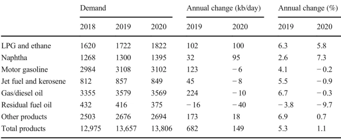
Over the same period, COVID-19 could have cut global emissions by 100 MtCO2(MtCO2) to date (see Figs.1and2), while China released around 400 MtCO2in 2019 whether the impacts of CO2emissions are diminished or reversed along, where the government’s response to the crisis is among the main aspects to consider (Table1). COVID-19 could cut 50% of global oil demand in January–September 2020 (IEA2020). Under the crisis scenario, the Chinese government’s policies and strategies, aimed to curb the disruption caused by COVID-19 outbreak, may balance these short-term impacts on energy and CO2emissions, the same way as was the case in the global financial crisis (GFC) and the internal economic slowdown in 2015.
The negative impact of the COVID-19 outbreak on energy consumption pattern will lead to a reduction in the emission of CO2emissions, as reported in the recent study of Zambrano-Monserrate et al. (2020). A decline in CO2emissions in de-veloped countries can also be said to be a consequence of the rise in services and information-intensive industries, instead of high-energy intensive and carbon-intensive industries (Huang et al. 2018). Before the COVID-19 lockdown, global CO2 emissions were expected to be like those in 2019, but the effect of confinement on CO2emissions are estimated to de-crease about 17% globally (Le Quéré et al.2020).
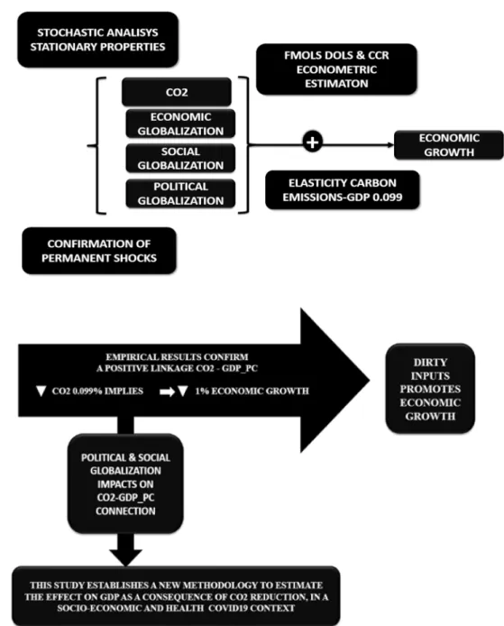
The present study seeks to analyze further the impact of COVID-19 outbreak over the Chinese economy. Hence, the focus is on determining the effects of the cut-offs of carbon emissions on Chinese economic growth during confinement. In doing so, carbon emissions are assumed to be dirty inputs. The lack of data implies adopting a strategy based on the study of stochastic process and elasticity, following a cointegration framework. These allow predicting the current situation and might be a proper tool for policymakers. Hence, econometric tools are used to determine the degree to which carbon emis-sions impact the Chinese economy and if the reduction in emissions levels will induce a decrease in income levels. This way, it is expected to identify warning signs, as well as to project the impacts of changes in carbon emission and globalization on the Chinese economy.
While carbon emissions and their implications are consid-ered in previous literature for testing the Environmental Kuznets Curve (Sidneva and Zivot2014), the present study assumes carbon emissions as a dirty input. It looks for how stationarity trend of carbon emissions helps to predict the adoption of new regulations. Furthermore, the study of Gil-Alana and Solarin (2018) outlined the variances between a trend and difference stationarity data generating process (DGP), which aid in ascertaining the possibility of long-run effects as it concerns environmental blueprints. As such, these approaches rely on the projection of forwarding pollutant emissions and affirming precision of the forecast. In addition, in the econometrics literature, dealing with stable and non-stable series, the long-term properties emanate from its
deterministic trend components. The series containing unit root generates uncertainty in the long term, while stationary (permanent) variables are free of uncertainty in GDP. On the contrary, modeling with non-stationary variable possess traits of uncertainty.
Three approaches are proposed for the Chinese economy: (1) examining the stationarity properties of the CO2emissions by both traditional and novel Fourier ADF-GLS, LM unit root test; (2) the linkage between economic growth and carbon emissions, under a globalization setting. Empirical outcomes might help policymakers on whether they should implement environmental restrictions. It would lead to reduce emissions or allow economic activities to address the pollution control automatically, where (3) cointegration is considered a suitable technique in this context based on the provision for elasticities
to induce the impact of carbon emissions over economic growth in China since December 2019, after confirmation of the first case of COVID-19 in Wuhan. This method will en-sure more flexibility in the dynamic specification of the mod-el. Furthermore, by considering globalization, additional in-formation about the nature of the shocks is included. Transitory isolation of the Chinese economy, both economic and social, as components of globalization, must be consid-ered for approximating to the real situation.
The structure of the paper is as follows: the second section reviews previous literature, the third section presents dataset and methodology, while the results of the analyses are pre-sented in the fourth section. The fifth section compiles the discussion of the findings, and the final section provides con-clusions and policy recommendations.
Fig. 1 Daily coal consumption at six major power firms in China (March 2020). Source: China Coal Transport & Distribution Association (2020), showing daily coal consumption for 6 major coastal power groups. Note: Right now, estimates are ranging between just under 60% and more than 70%. Bloomberg (2020):https://www.bloomberg. com/news/articles/2020-03-05/a- new-number-to-watch-for-china-s-economy-the-resumption-rate
Fig. 2 Greenhouse gas emissions in China. Source: The European Space Agency (2020). Note: The decline in economic activity in China is now visible from space. This trend is confirmed in China’s big cities. In the second half of February, there was no activity
Literature review
Limited studies exist on the stationarity assessment of carbon emissions. Reviews by Aldy (2006) or Lee and Chang (2009) have explored the carbon emissions movement of the devel-oped, and industrialized countries and non-stability of the de-veloping countries was assessed through the stationarity test-ing procedure proposed by Carrion-i-Silvestre et al. (2009). Several studies tested the stationarity properties of carbon emissions (e.g., Romero-Avila2008; Ahmed et al. 2016). Christidou et al. (2013) applied a non-linear panel unit root test confirming the stationary for 33 nations during 1870– 2006. On the other hand, there is an impressive entirety of papers that provide the proof for the non-stationary of carbon discharges (Criado and Grether2011). Different investiga-tions confirm that carbon emanainvestiga-tions follow unit root process (Li and Lin2013; Presno et al.2018). Under these outcomes, Jaunky (2011) demonstrated that CO2emissions for high-earning nations are I(1) integrated. Yamazaki et al. (2014) indicated that in the OECD countries, per capita CO2 emis-sions follow unit root. Barros et al. (2016) applied fragmen-tary combination for the global series of carbon discharges and arrangement of every one of its five segments (gas, fluids, solids, concrete creation, and gas flaring). The observational outcomes indicated that the arrangement is non-stationary with the integration order fundamentally over 1.
Furthermore, on the literature trajectory between globaliza-tion, energy consumpglobaliza-tion, and economic growth, several stud-ies analyzed the relationship between globalization, energy consumption, and economic growth (see Solarin et al.2016; Alola et al.2019; Wu et al. 2019). However, studies have ignored mainly a various aspect of globalization, i.e., political globalization, social globalization, and economic globalization. Solarin et al. (2016) discovered that there exists a positive correlation between globalization and energy con-sumption in the long term. Energy concon-sumption, urbanization, financial development, and economic growth have positive effects on emissions, in the presence of globalization. On the
contrary, openness to trade, foreign direct investment, and innovation have exhibited negative impacts on emissions, as reported by Shahbaz et al. (2019).
Furthermore, Alola et al. (2019) show that energy con-sumption is strongly related to globalization in the long run while adopting the Autoregressive distributed lag approach. Tourism can be considered a form of social globalization, which promotes CO2emissions in both the short and long term, while the real income and level of globalization promote CO2emissions only in the long term. Thus, ensuring the sus-tainability of global energy use, it is pertinent to shift from import-oriented economies to export-based economies.
In addition, export-oriented and emerging economies, such as China, need to adjust trade pattern to ensure economic and ecological competence in the global market, aside from im-proving production efficiencies (Wu et al.2019). As energy is an essential factor for economic growth, its conservation may harm growth pattern (Ouedraogo2013).
Furthermore, tourism exposure, as a consequence of the globalization process, and the amount of energy consumed is in long-run equilibrium relationship with CO2emissions. Development of tourism has led not only to a considerable increase in energy use but also to climate change (Katircioglu2014, Katircioglu et al.2020). Energy consump-tion, level of real income/output, and globalization play essen-tial roles in achieving environmental sustainability. Trade openness leads to an increase in globalization while having an inverse impact on pollution (Akadiri et al.2019).
While considering the effects of carbon emissions associ-ated with consumption of electricity from non-renewable sources, Apergis and Payne (2012) found a unidirectional causal relationship between economic growth and renewable electricity consumption in the short run and bidirectional cau-sality between them in the long run. Second, there exists a two-way causal relationship between non-renewable electric-ity consumption and economic growth both in the short and long run. Economic growth has a positive and statistically significant effect on energy consumption in the short run.
Table 1 Chinese demand by-product (thousand barrels per day)
Demand Annual change (kb/day) Annual change (%) 2018 2019 2020 2019 2020 2019 2020 LPG and ethane 1620 1722 1822 102 100 6.3 5.8
Naphtha 1268 1300 1395 32 95 2.6 7.3
Motor gasoline 2984 3108 3102 123 − 6 4.1 − 0.2 Jet fuel and kerosene 812 857 849 45 − 8 5.5 − 0.9 Gas/diesel oil 3355 3579 3569 224 − 10 6.7 − 0.3 Residual fuel oil 432 416 375 − 16 − 40 − 3.8 − 9.7 Other products 2503 2676 2694 173 18 6.9 0.7 Total products 12,975 13,657 13,806 682 149 5.3 1.1 Source: IEA (2020)
An increase in real GDP is likely to affect energy demand since energy is a considerable input in the production process (Ouedraogo2013). Finally, there is a positive correlation be-tween globalization and energy consumption in the long term (Solarin et al.2016). To our knowledge, no study has looked at the influence of the COVID-19 outbreak on energy con-sumption, economic growth, and globalization. This process is what the present study is aimed at investigating.
Empirical methodology and data
Over the last decade, the Chinese economy has been plagued with air pollution (Zhang et al.2014) due to massive industri-alization and anthropogenic activities. To this end, the present study attempts to validate a direct relationship between eco-nomic growth and carbon emissions in China between 1981 and 2014, to establish the elasticity relationship between car-bon emissions and economic growth for policy formulation. We also explore the impact of economic, social, and political globalization on economic growth, and the effect of confine-ment, isolating both economic and social globalization. We assume that carbon emissions, as dirty input (Emir and Bekun
2019), exert a direct impact over economic growth. In other words, we expect to confirm that rising carbon emissions will lead to ascending economic growth (Balsalobre et al.2020) to determine the elasticity relationship between these variables and induce the impact of the reduction in carbon emissions on economic growth in China during 2020 confinement. To strengthen the model toward a closed economy, the empirical model proposes the omission of the economic and social glob-alization variables, which are more related to the movement of people, businesses, intermediate goods, and raw materials.
On the premise of the highlighted literature, the present study is also motivated by the campaign of United Nations Sustainable Development Goals (UN-SDG-3, 8, 11, 13, and 17) that borders around sustainability, good health, economic expansion, climate change mitigation issues, and global part-nership in the context of our study. The SDGs informed the construction of variables adopted for the econometric analy-sis, and subsequently, the following hypotheses were present-ed to tie study aim properly:
H1: There is a direct connection between per capita CO2 and per capita GDP in China.
The present study seeks to underpin if economic activities in a highly industrialized nation (such as China) trigger pollu-tion emission. In addipollu-tion, several studies have validated the relationship (Adedoyin et al.2020) without considering the interconnectedness of countries. This validation led to the construction of the next hypothesis:
H2: There is a direct linkage between globalization and economic growth. According to the UN-SDG-17 that outlined the role of partnership for sustainability, the present study seeks to understand the directional nature of connection in a cointegrated framework for China. H3: The economic and social isolation, as a consequence of the COVID-19 pandemic, present an adverse effect over the Chinese economic growth.
This hypothesis is in line with UN-SDG-3, where the em-phasis is placed on sustainable health for national prosperity. In the context of the global pandemic for the case of China, the present study seeks to understand the effect of social isolation and its implications on economic growth while considering health status.
For testing these hypotheses, we propose two models (Eqs.
1and2), as follows:
LGDPt¼ α0þ α1LCO2tþ α3LEGtþ α4LSGt
þ α5LSPtþ εit ð1Þ
Equation 1 contains logarithm expression of per capita gross domestic product— LGDPt, and per capita carbon emis-sions—LCO2t−(World Bank2020), considered as dirty input, to investigate the relationship between these variables. Equation1also includes the economic (LEGt), social (LSGt), and political (LPGt)globalization (KOF2020) in logarithm form.
Our primary model (Eq.2) represents the effects of both economic and social globalization are isolated, to understand the lockdown assumed for Chinese Administration during COVID-19 crisis:
LGDPt¼ α0þ a1LCO2tþ a5LSPtþ εit ð2Þ An essential aspect of the present study is to validate the existence of a decoupling that varies over time and therefore invalidates the long-term predictions. To do this, we first an-alyze the processes and stochastic properties of the variables used. In consequence, we need to examine the stationarity properties of the selected variables to formulate long-term policy implications. In time series analysis, changes in a mod-el parameter in temporal stationarity signifies that variance and average are constant. In consequence, we assume that when a model parameter alters its individual projected value and the mean, policy-level shocks have no permanent impact on them, and those shocks are not sturdy. However, in case a model parameter demonstrates non-stationarity, policies lean-ing toward adoptlean-ing that parameter will be useful (Perron
1989). Consequently, policy-level standpoint requires to be deliberated to the tenure of the effect.
In the incidence of stationarity, every policy shock needs not to endure transitory impact, or they might not prove to be
impactful. Fleeting policies—the ones to alter the capacity of applicable model parameters—will be likely to demonstrate individual momentary impacts. Perpetual fluctuations conse-quently call for a more enduring policy-level standpoint in a condition of this kind. Conversely, in the incidence of non-stationarity, transitory shocks will demonstrate lasting impacts (Belbute and Pereira2017).
The present study follows this methodology; if unit root analysis is suitable for checking stationarity properties of the series and in consequence, it will disclose appropriate policy recommendations. Even traditional unit root tests—ADF test (Dickey and Fuller1981), PP test (Phillips and Perron1988), KPSS test (Kwiatkowski et al.1992), DF-GLS test (Elliott et al.1996), or NP test (Ng and Perron2001)—follow their
test procedures; these tests are likely to assent to the null hypothesis that is mostly grounded on the presence of unit root, while the model parameters contain structural breaks (Perron1989). Another unit root tests by Lee and Strazicich (2003) recommend a bi-break lowest Lagrange multiplier (LM) unit root test, with alternative hypothesis unequivocally inferring trend stationarity.
Furthermore, Zivot and Andrews (1992) (ZA) and Lumsdaine and Papell (1997) (LP) unit root tests ponder upon the same number of structural breaks. Also, ZA and LP un-dertake no breaks as the null hypothesis, while stemming the critical points. Accordingly, alternative hypothesis signifies the persistence of structural breaks, although model parame-ters might demonstrate non-stationarity. Consequently, LM test admits breaks and deliberates the occurrence of unit root where the ideal count of breaks is endogenously governed. Hence, LM test outcome is more agreeable in the incidence of two structural breaks. In econometric literature, we also find a variant of Gallant’s (1981) Flexible Fourier Form, Enders and Lee (2012a, 2012b), or Rodrigues and Taylor (2012) proposed Fourier unit root test, where, rather than choosing specific break periods, their count, and arrangement, the measurement issue is transmuted into slotting in the appli-cable frequency modules within the empirical model (Enders and Lee2012b).
So, Fourier unit root tests count on estimations while de-liberating deviances from the average in measurable expres-sions using trigonometric expresexpres-sions. In the pursuit, Enders and Lee (2012a) applied LM regression, which was promoted initially by Schmidt and Phillips (1992). On the other hand, Rodrigues and Taylor (2012) opted for GLS regression based on Elliott et al. (1996), while Enders and Lee (2012b) e m p l o y e d D i c k e y a n d F u l l e r (1 9 8 1) r e g r e s s i o n . Consequently, these estimation procedures will be recognized as Fourier LM, Fourier GLS, and Fourier ADF, correspond-ingly. Once we have checked the stochastic properties of the proposed variables to be allowed to establish long-run policy recommendations, the primary aim of the present paper is to estimate the emissions–GDP elasticities (Cohen et al.2018),
so as to establish a robust pattern for considering how the reduction in emissions will infer over economic growth, via long-run elasticities. Cohen et al. (2018) used the standard decomposition cycle or trend used in many other fields of economics. A panel cointegration model was used by Narayan and Narayan (2010) to evaluate the elasticities of emissions in the short and long run as regards the developing economies’ output.
Fisher–Johansen’s cointegration test (1991) joins separate estimation procedures while associating estimation proce-dures from distinct cross-sections.Πiis thep value of a spe-cific cointegration module for cross-section i. The null hy-pothesis for the panel thus turns out to be
−2∑N
i¼1logð Þ→χΠi 22N ð3Þ
χ2 values are built upon MacKinnon–Haug–Michelis (1999), and p values are calculated by Johansen’s cointegration trace and maximum eigenvalue tests.
FMOLS (fully modified least squares) and the DOLS (dy-namic ordinary least squares) methods are used for validating the hypotheses. These econometric methods can tackle the endogeneity and serial correlation issues. They are also valid for samples with lesser size by disregarding inaccuracy caused by sample bias (Narayan and Narayan2005).
Empirical results and discussions
This section presents and interprets the study’s empirical re-sults, as highlighted in the“Empirical methodology and data” section. These sections proceed with tests of variables station-arity properties and subsequent tests accordingly.
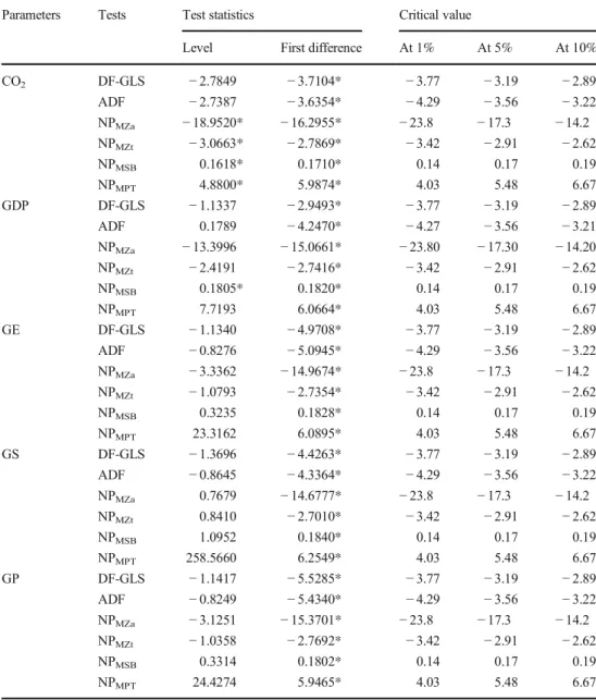
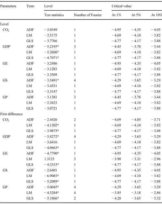
As the starting point of the analysis, we have analyzed the unit root properties of the model parameters, and in this pur-suit, we have employed the DF-GLS, ADF, and LM unit root tests, and the test outcomes are recorded in Table2. The test outcome divulges that the model parameters are stationary after first difference, and thereby indicating their order on integration to be unity. However, these tests cannot produce a robust outcome in the presence of unknown structural breaks, and therefore, we have employed Fourier unit root test (see Table3). The result of Fourier unit root test divulges that the model parameters are integrated into the presence of struc-tural breaks. From empirical results, we can induce the select-ed variables for prselect-edicting long-term effect.
In consequence, the stationarity properties of carbon emis-sions determine whether the policies will be useful or not. Our study also presents limitations, as we are not considering the technical effect (Alvarez et al.2017) and the effects of renew-able energy use. However, the present study focuses on the carbon emissions–GDP elasticities and how the absence of the globalization process infers. In consequence, our empirical
results (Tables2 and3) may be misleading to make policy recommendations if we only consider carbon emissions– economic growth consequence. Therefore, we also consider the effects of economic, social, and political globalization, and absence of economic and social globalization caused by so-cioeconomic isolation imposed by the Chinese authorities as a result of the COVID-19 outbreak.
Subsequently, we have obtained evidence of a long-term relationship that allows us to make recommendations that are more than temporary in nature. The next step is to estimate the connection between carbon emissions and economic growth through cointegration. To proceed, we need to confirm the long-run relationship between proposed variables through cointegration tests (see Table4).
After ascertaining the long-run association among the mod-el parameters, three different tests are applied: fully modified
ordinary least squares (FMOLS) suggested by Phillips and Hansen (1990), dynamic ordinary least squares (DOLS) pro-posed by Saikkonen (1991) and Stock and Watson (1993), and conical cointegration regression (CCR) based on Park (1992). This battery of tests is capable of endowing us with consistent and robust test outcomes, given the small volume of data. FMOLS outcomes are robust in the presence of serial correlation and endogeneity, which might be arising out of the probable cointegrating association among the model parame-ters (Phillips 1995), while DOLS allows the elimination of possible feedback persistent in the cointegrating association among the model parameters.
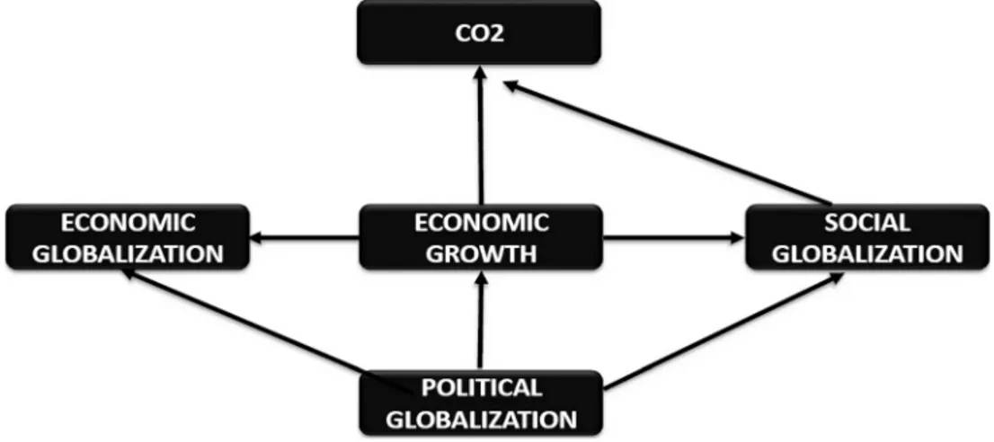
The results of causality analysis (Table5) highlight the degree of predictability of each variable on another. A one-way causal relationship between economic and social global-ization and CO2emissions is endorsed. This result suggests
Table 2 Traditional unit root test
outcome Parameters Tests Test statistics Critical value
Level First difference At 1% At 5% At 10% CO2 DF-GLS − 2.7849 − 3.7104* − 3.77 − 3.19 − 2.89 ADF − 2.7387 − 3.6354* − 4.29 − 3.56 − 3.22 NPMZa − 18.9520* − 16.2955* − 23.8 − 17.3 − 14.2 NPMZt − 3.0663* − 2.7869* − 3.42 − 2.91 − 2.62 NPMSB 0.1618* 0.1710* 0.14 0.17 0.19 NPMPT 4.8800* 5.9874* 4.03 5.48 6.67 GDP DF-GLS − 1.1337 − 2.9493* − 3.77 − 3.19 − 2.89 ADF 0.1789 − 4.2470* − 4.27 − 3.56 − 3.21 NPMZa − 13.3996 − 15.0661* − 23.80 − 17.30 − 14.20 NPMZt − 2.4191 − 2.7416* − 3.42 − 2.91 − 2.62 NPMSB 0.1805* 0.1820* 0.14 0.17 0.19 NPMPT 7.7193 6.0664* 4.03 5.48 6.67 GE DF-GLS − 1.1340 − 4.9708* − 3.77 − 3.19 − 2.89 ADF − 0.8276 − 5.0945* − 4.29 − 3.56 − 3.22 NPMZa − 3.3362 − 14.9674* − 23.8 − 17.3 − 14.2 NPMZt − 1.0793 − 2.7354* − 3.42 − 2.91 − 2.62 NPMSB 0.3235 0.1828* 0.14 0.17 0.19 NPMPT 23.3162 6.0895* 4.03 5.48 6.67 GS DF-GLS − 1.3696 − 4.4263* − 3.77 − 3.19 − 2.89 ADF − 0.8645 − 4.3364* − 4.29 − 3.56 − 3.22 NPMZa 0.7679 − 14.6777* − 23.8 − 17.3 − 14.2 NPMZt 0.8410 − 2.7010* − 3.42 − 2.91 − 2.62 NPMSB 1.0952 0.1840* 0.14 0.17 0.19 NPMPT 258.5660 6.2549* 4.03 5.48 6.67 GP DF-GLS − 1.1417 − 5.5285* − 3.77 − 3.19 − 2.89 ADF − 0.8249 − 5.4340* − 4.29 − 3.56 − 3.22 NPMZa − 3.1251 − 15.3701* − 23.8 − 17.3 − 14.2 NPMZt − 1.0358 − 2.7692* − 3.42 − 2.91 − 2.62 NPMSB 0.3314 0.1802* 0.14 0.17 0.19 NPMPT 24.4274 5.9465* 4.03 5.48 6.67 *Signifies stationarity
that economic and social integration with the rest of the world drives CO2 emissions over the sampled period. However, there is a deviation since December 2019, after the first case of the COVID-19 was reported in Wuhan. These translate into low emissions level over the recent months. This outcome resonates the novel and recent findings of Zambrano-Monserrate et al. (2020). However, this finding has further impact given the isolation of China from the rest of the world to ameliorate the health issues, which also have its environ-mental implication. These revelations are suitable for proper policy contrition with synergy with other macroeconomic in-dicators of China. Further insights on causality results are highlighted in Fig.3.
Table 3 Fourier ADF, LM, and
GLS unit root test outcome Parameters Tests Level Critical value
Test statistics Number of Fourier At 1% At 5% At 10% Level CO2 ADF − 3.0349 1 − 4.95 − 4.35 − 4.05 LM − 3.5175 1 − 4.69 − 4.10 − 3.82 GLS − 3.7766 1 − 4.77 − 4.17 − 3.88 GDP ADF − 5.2195* 3 − 4.45 − 3.78 − 3.44 LM − 5.2606* 1 − 4.69 − 4.10 − 3.82 GLS − 4.7071* 1 − 4.77 − 4.17 − 3.88 GE ADF − 3.2486 1 − 4.95 − 4.35 − 4.05 LM − 3.1283 1 − 4.69 − 4.10 − 3.82 GLS − 3.3508 1 − 4.77 − 4.17 − 3.88 GS ADF − 3.5491* 4 − 4.29 − 3.65 − 3.29 LM − 3.4531 1 − 4.69 − 4.10 − 3.82 GLS − 3.3147 1 − 4.77 − 4.17 − 3.88 GP ADF − 3.1381 3 − 4.45 − 3.78 − 3.44 LM − 2.2623 1 − 4.69 − 4.10 − 3.82 GLS − 3.0721 1 − 4.77 − 4.17 − 3.88 First difference CO2 ADF − 2.4426 2 − 4.69 − 4.05 − 3.71 LM − 4.1202* 1 − 4.69 − 4.10 − 3.82 GLS − 3.9875* 1 − 4.77 − 4.17 − 3.88 GDP ADF − 5.8272* 4 − 4.29 − 3.65 − 3.29 LM − 3.6416 1 − 4.69 − 4.10 − 3.82 GLS − 4.0663* 1 − 4.77 − 4.17 − 3.88 GE ADF − 4.7790* 1 − 4.95 − 4.35 − 4.05 LM 1.3125 3 − 3.98 − 3.31 − 2.96 GLS − 4.3315* 1 − 4.77 − 4.17 − 3.88 GS ADF − 2.6401 1 − 4.95 − 4.35 − 4.05 LM − 6.9083* 1 − 4.69 − 4.10 − 3.82 GLS − 5.2089* 1 − 4.77 − 4.17 − 3.88 GP ADF − 5.0045* 4 − 4.29 − 3.65 − 3.29 LM − 4.5284* 4 − 3.85 − 3.18 − 2.86 GLS − 5.1866* 2 − 4.28 − 3.65 − 3.32 *Signifies stationarity
Table 4 Cointegration test results Unrestricted cointegration rank test (trace) Hypothesized Trace 0.05
Number of CE(s) Eigenvalue Statistic Critical value Probability r ≤ 0 0.756518*** 116.3903 69.81889 (0.0000) r ≤ 1 0.670621*** 72.59616 47.85613 (0.0001) r ≤ 2 0.493293*** 38.16927 29.79707 (0.0043) r ≤ 3 0.283929** 17.09479 15.49471 (0.0285) r ≤ 4 0.195448*** 6.741543 3.841466 (0.0094) 5 cointegrating vectors are considered; ***, **, and * represent statistical level of significance value at 1, 5, and 10%, respectively
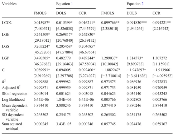
Table6shows all the values obtained from the FMOLS, DOLS, and CCR estimations for the proposed Eqs.1and2. The empirical results confirm the direct connection between selected explanatory variables (CO2, EG, SG, PG) and eco-nomic growth (LGDP). At the same time, Eq.1 considers globalization process, and in Eq.2, we omit the impact of economic and social globalization (we found that political globalization is maintained during COVID-19 crisis).
The outcome of Eqs. 1 and 2 across three methodo-logical procedures demonstrate that CO2 emissions have
a direct impact on the GDP. If we compare both models, we can observe that when we isolate the effects of both economic and social globalization, the connec-tion between carbon emissions and economic growth is higher (0.099766), and even the explanatory power of the adjusted R2 has been reduced (Fig. 4). The primary concern, however, is to find the nature of GDP and CO2 relationship under a confinement scenario, which explains that an increase in 1% of carbon emissions (considered as dirty input) (Balsalobre et al. 2020) will increase economic growth by 0.09%. This result evi-dences that the Chinese economy is inelastic to econom-ic growth in the presence of economeconom-ic and social isola-tion. Interestingly, the long-run regression of DOLS, FMOLS, and CCR all resonates higher magnitudes of the impact of political willpower of dirty economic rel-ative to model (1) with the interaction with rest of the world by the incorporation of the economic and social dimension of globalization as reported in Table 6.
These results suggest that the Chinese economy does not respond to pollutant emission over the sampled peri-od. This outcome echoes the study of Emir and Bekun (2019) for the case of Romania. Table 5 reports the cau-sality analysis over the outlined variables. We see a uni-directional causality running from economic globalization to CO2 emissions. Similarly, one-way causality is ob-served between social globalization and CO2 emissions, while no causality is seen between political globalization and CO2emissions. These results help us understand the predictive power of one variable over another. We ob-serve that both social and economic interaction of eco-nomics response to increases in pollution economy. At the same time, political willpower is crucial to mitigating pollution economy, which has been demonstrated in the current study as no causal interaction is seen between economic growth and CO2. The plausible explanation could be the current disposition of the Chinese economy to be insulated from the rest of the nations.
Fig. 3 Pairwise Granger causality tests scheme
Table 5 Causality test results
Null hypothesis: Observed F statistic Probability LGDP≠> LCO2 32 1.659** (0.04855) LCO2≠> LGDP 0.329 (0.37095) LGE≠> LCO2 32 4.54151** (0.0417) LCO2≠> LGE 1.22505 (0.2775) LGP≠> LCO2 32 0.39555 (0.5343) LCO2≠> LGP 0.05798 (0.8114) LGS≠> LCO2 32 3.39011* (0.0758) LCO2≠> LGS 1.99034 (0.1689) LGE≠> LGDP 32 1.04018 (0.3162) LGDP≠> LGE 6.11637** (0.0195) LGP≠> LGDP 32 3.37740* (0.0764) LGDP≠> LGP 0.12886 (0.7222) LGS≠> LGDP 32 0.83329 (0.3689) LGDP≠> LGS 6.87025* (0.0138) LGP≠> LGE 32 5.90930** (0.0215) LGE≠> LGP 0.00978 (0.9219) LGS≠> LGE 32 1.53949 (0.2246) LGE≠> LGS 2.13349 (0.1549) LGS≠> LGP 32 0.20806 (0.6517) LGP≠> LGS 11.3896*** (0.0021) ***, **, and * represent statistical level of significance value at 1%, 5%, and 10% respectively. Here≠> means “Granger cause another” the null hypothesis for the causality test
Conclusion and policy implications
In more recent times, the world has experienced several un-certainties ranging from the Great Depression in the 1930s, Global Food Crises of 2006 to the Great Recession burn of the global financial crisis (2008–2009) to the very recent pandem-ic of COVID-19, whpandem-ich stem from the Republpandem-ic of China at Wuhan. As an extreme event, the outbreak of COVID-19 has damaged the global economic growth generating a specific impact on the environment. The COVID-19 pandemic has radically altered patterns of energy demand in both China and around the rest of the world. Current estimations have assessed the decrease in CO2emissions during forced confine-ments. These mentioned uncertainties have a ripple effect on socioeconomic and macroeconomic indicators of any nation. Thus, given the current happening and isolation of the Republic of China from the rest of the community of nations to mitigate the effect of the COVID-19 pandemic, we focus on the Chinese economy. For testing the highlighted hypotheses proposed in the present study, conventional and current econometrics tools were adopted over annual time frequency from 1981 to 2014. Assuming that COVID-19 significantly has reduced the concentration of emission in the atmosphere (Wang and Su2020), the empirical estimation traces and val-idates the cointegration relationship between economic
growth and pollutant emission (CO2), all dimensions of glob-alization (social, economic, and political) in China oversampled period. The long-run regressions of DOLS, FMOLS, and CCR validate a positive and inelastic relation-ship between economic growth and pollutant emission in China. This outcome is indicative to government officials of China, as it implies that the Chinese economy is not respon-sive to dirty (CO2) economic growth. This is seen in the re-duction of pollutant emissions in recent times because of less industrial activities that pollute the environment (see Fig.1for more insights into this argument). This position of carbon reduction admits COVID resonates the recent declaration by the report of Carbon Brief about the reduction of CO2 emis-sions based on the decline in coal consumption.
Furthermore, the current study constructed twin models, where model 2 is the baseline, focused on the isolation effects of both social and economic globalization on economic growth in recent time. The regression indicates that the polit-ical willpower of the government administrators of Chinese economy to curb the wild spread of health challenges that cut across the globe. This is endorsed by the positive and elastic effect of the political wave of globalization to economic growth. Thus, despite the Chinese economy isolation from the rest of the world, economic growth was still experienced, given the positive and significant growth trajectory (see
Table 6 FMOLS, DOLS, and CCR estimation of long-run coefficient
Variables Equation1 Equation2
FMOLS DOLS CCR FMOLS DOLS CCR
LCO2 0.015987* 0.015399* 0.016211* 0.099766** 0.091830*** 0.094221** [7.480671] [6.526038] [7.445579] [2.385010] [1.944264] [2.216742] LGE 0.261509* 0.269817* 0.262830* [29.18012] [20.76840] [26.39132] LGS 0.205224* 0.205458* 0.204685* [45.23206] [47.57804] [46.67654] LGP 0.490505* 0.482779 0.489244* 1.299037* 1.314573* 1.307272 [46.37683] [29.16463] [47.58904] [10.30842] [9.890783] [11.15901] C 0.089991* 0.094005 0.092400* − 1.882247* − 1.947697* − 1.913966 [2.919269] [2.297708] [3.274027] [− 3.718014] [− 3.611626] [− 4.095952] R2 0.999888 0.999982 0.999887 0.973575 0.986936 0.972833 AdjustedR2 0.999871 0.999959 0.999871 0.971753 0.981959 0.970959 SE of regression 0.003014 0.001624 0.003018 0.044623 0.034140 0.045245 Log likelihood 6.45E−06 1.84E−06 6.45E−06 0.003766 0.002808 0.003766 Mean dependent variable 3.874410 3.880246 3.874410 3.874410 3.880246 3.874410 SD dependent variable 0.265502 0.254175 0.265502 0.265502 0.254175 0.265502 Sum squared residual 0.000245 3.43E−05 0.000246 0.057745 0.024476 0.059367 Dependent variable:LGDP (1981–2014)
Table 6). However, the more inclusive model displays a significant impact of social and economic globalization on Chinese economic growth as confirmed by the causality analysis; both economic and social globalization predicts pollutant emissions. This result suggests that interaction with the rest of the world contains externalities directly connected with the environment. It is worth mentioning that isolation from the rest of the world does not show any causality with pollutant emission in the present study. These calls for intensive policy mix linked to the environ-ment, as isolation from the rest of the world has its im-plications, and given the trade-off between economic growth and pollutant emissions, there is a need for caution when liberalizing the economy, as well as strong political
willpower aiming to mitigate the adverse effect of global-ization at all time.
Recent studies (Le Quéré et al.2020; Wang and Su2020) confirm the reduction in emissions in China since the begin-ning of COVID-19 crisis, as result of the implementation of strict confinement measure amend the spread of the virus at both national and international level (e.g., restrictions on trade and international tourism). This should shorten the spread of the pandemic. However, the laydown restrictions come with some economic (negative) implications.
While OECD countries are expected to register an econom-ic decrease of their real GDP between 7.5 and 9.3% depending on single- or double-hit scenario caused by COVID-19 crisis, China presents a more optimistic situation with a range of
Fig. 4 FMOLS, DOLS, and CCR estimation results scheme
decrease between 2.6 and 3.7% (OECD2020). These projec-tions are in line with our study results for the Chinese econo-my. Even this research on COVID-19 crisis was in full swing, and limitations were faced for such an analysis. Despite this, our study aims to establish a methodology that serves as a tool for predicting the economic impact of COVID-19 not just in China but globally. Obtaining data on the reduction of emissions monthly allows us to adapt the growth forecasts according to the levels of CO2, under a model that has considered the isolation caused by this crisis and its effects for the economy. Moreover, this methodology might be considered for other economies strongly affected by COVID-19 (e.g., EU, USA, Brazil, or India), but also for more local predictions regarding the levels of water pollution (PME) or the levels of NO2or GHG.
The current study is not void of policy direction for all stakeholders and the government administrator in China. The isolation of the Chinese economy from the rest of the world makes both conventional and health sense. This action is timely and worthwhile to help flatten the rise of the spread of COVID-19 and after that, reduce the working and active (workforce) population as results of infection from the virus. We observe that the willpower of the Chinese government is significant, and there is no causality between political global-ization and pollutant emission against contract expectation where both social and economic globalizations engender CO2emissions. The current study employed the government of the day to sustain the current momentum.
References
Adedoyin FF, Gumede MI, Bekun FV, Etokakpan MU, Balsalobre-Lorente D (2020) Modelling coal rent, economic growth and CO2
emissions: does regulatory quality matter in BRICS economies? Sci Total Environ 710:136284
Ahmed M, Khan AM, Bibi S (2016) Convergence of per capita CO2
emissions across the globe: insights via wavelet analysis. Renew Sust Energ Rev 75:86–97
Akadiri AC, Akadiri S, Saint GH (2019) The role of natural gas consump-tion in Saudi Arabia’s output and its implicaconsump-tion for trade and envi-ronmental quality. Energy Policy 129:230–238
Aldy JE (2006) Per capita carbon dioxide emissions: convergence or divergence? Environ Resour Econ 33:533–555
Alola AA, Yalçiner K, Alola UV, Akadiri S (2019) The role of renewable energy, immigration and real income in environmental sustainability target. Evidence from Europe largest states. Sci Total Environ 674: 307–315
Alvarez HA, Balsalobre D, Shahbaz M, Cantos JM (2017) Energy inno-vation and renewable energy consumption in the correction of air pollution levels. Energy Policy 105:386–397
Apergis N, Payne JE (2012) Renewable and non-renewable energy consumption-growth nexus: Evidence from a panel error correction model. Energy Econ 34(3):733–738
Balsalobre-Lorente D, Driha OM, Shahbaz M, Sinha A (2020) The ef-fects of tourism and globalization over environmental degradation in developed countries. Environ Sci Pollut Res 27(7):7130–7144
Barros CP, Gil-Alana LA, De Gracia FP (2016) Stationarity and long-range dependence of carbon dioxide emissions: evidence for disag-gregated data. Environ Resour Econ 6:45–56
Belbute JM, Pereira AM (2017) Do global CO2emissions from fossil-fuel
consumption exhibit long memory? A fractional-integration analy-sis. Appl Econ 49(40):4055–4070
Carrion-i-Silvestre JL, Kim D, Perron P (2009) GLS-based unit root tests with multiple structural breaks under both the null and the alterna-tive hypotheses. Economic Theory 25(6):1754–1792
Christidou M, Panagiotidis T, Sharma A (2013) On the stationarity of per capita carbon dioxide emissions over a century. Econ Model 33: 918–925
Cohen G, Jalles JT, Loungani P, Marto R (2018) The long-run decoupling of emissions and output: evidence from the largest emit-ters. Energy Policy 118:58–68
Criado CO, Grether JM (2011) Convergence in per capita CO2emissions:
a robust distributional approach. Resour Energy Econ 33:637–665 Dickey BYDA, Fuller WA (1981) Likelihood ratio statistics for
autoregressive time series with a unit root. Econometrica 49(4): 1057–1072
Elliott G, Rothenberg TJ, Stock JH (1996) Efficient tests for an autoregressive unit root. Econometrica. 64:813–836
Emir F, Bekun FV (2019) Energy intensity, carbon emissions, renewable energy, and economic growth nexus: new insights from Romania. Energy Environ 30(3):427–443
Enders W, Lee J (2012a) A unit root test using a Fourier series to approx-imate smooth breaks. Oxf Bull Econ Stat 74(4):574–599
Enders W, Lee J (2012b) The flexible Fourier form and Dickey–Fuller type unit root tests. Econ Lett 117(1):196–199
European Space Agency, (2020). COVID-19: nitrogen dioxide over China.https://www.esa.int/Applications/Observing_the_Earth/ Copernicus/Sentinel-5P/COVID-19_nitrogen_dioxide_over_China
(Accessed June 2020)
Fernandes N (2020) Economic effects of coronavirus outbreak (COVID-19) on the world economy. Available at SSRN 3557504. Gil-Alana LA, Solarin SA (2018) Have US environmental policies been
effective in the reduction of US emissions? A new approach using fractional integration. Atmos Pollut Res 9:53–60
Huang WJ, Hung K, Chen CC (2018) Attachment to the home country or hometown? Examining diaspora tourism across migrant genera-tions. Tour Manag 68:52–65
IEA (2020). Oil Market Report—March 2020. Retrieved fromhttps:// www.iea.org/reports/oil-market-report-march-2020, March 2020. Jaunky V (2011) The CO2emissions–income nexus: evidence from rich
countries. Energy Policy 39:1228–1240
Katircioglu ST (2014) International tourism, energy consumption, and environmental pollution: the case of Turkey. Renew Sust Energ Rev 36:180–187
Katircioglu ST, Saqib N, Katircioglu S, Kilinc CC, Gul H (2020) Estimating the effects of tourism growth on emission pollutants: empirical evidence from a small island, Cyprus. Air Qual Atmos Health 13:1–7
Keogh-Brown MR, Smith RD (2008) The economic impact of SARS: how does the reality match the predictions? Health Policy 88(1): 110–120
KOF Swiss Economic Institute, KOF Globalisation Index (2020) Retrieved fromhttps://kof.ethz.ch/en/forecasts-and-indicators/ indicators/kof-globalisation-index.html
Kwiatkowski D, Phillips PCB, Schmidt P, Shin Y (1992) Testing the null hypothesis of stationarity against the alternative of a unit root. How sure are we that economic time series have a unit root? J Econ 54(1-3):159–178
Le Quéré C, Jackson RB, Jones MW, Smith AJ, Abernethy S, Andrew RM et al (2020) Temporary reduction in daily global CO2 emissions during the COVID-19 forced confinement. Nat Clim Chang 10:1–7
Lee CC, Chang CP (2009) Stochastic convergence of per capita carbon dioxide emissions and multiple structural breaks in OECD countries. Econ Model 26:1375–1381
Lee J, Strazicich MC (2003) Minimum Lagrange multiplier unit root test with two structural breaks. Rev Econ Stat 85(4):1082–1089 Leiva-Leon D, Perez-Quiros G, Rots E (2020) Real-time weakness of the
global economy: a first assessment of the coronavirus crisis. Working Paper Series 2381. European Central Bank.
Li X, Lin B (2013) Global convergence in per capita CO2emissions.
Renew Sust Energ Rev 24):357–363
Lumsdaine RL, Papell DH (1997) Multiple trend breaks and the unit-root hypothesis. Rev Econ Stat 79(2):212–218
MacKinnon JG, Haug AA, Michelis L (1999) Numerical distribution functions of likelihood ratio tests for cointegration. J Appl Econom 14(5):563–577
Narayan PK, Narayan S (2005) Estimating income and price elasticities of imports for Fiji in a cointegration framework. Econ Model 22(3): 423–438
Narayan P, Narayan S (2010) Carbon dioxide emissions and economic growth: panel data evidence from developing countries. Energy Policy 38(1):661–666
Ng S, Perron P (2001) A note on the selection of time series models. Working Papers in Economics, 116.
OECD (2020). Coronavirus: the world economy at risk. OECD Interim Economic Assessment. Retrieved from https://www.oecd.org/ berlin/publikationen/Interim-Economic-Assessment-2-March-2020.pdf, April 2020
Ouedraogo NS (2013) Energy consumption and economic growth: evi-dence from the Economic Community of West African States (ECOWAS). Energy Econ 36:637–647
Park JY (1992) Canonical cointegrating regressions. Econometrica. 60(1):119–143
Perron P (1989) The great crash, the oil price shock, and the unit root hypothesis. Econometrica. 57(6):1361–1401
Phillips PC, Perron P (1988) Testing for a unit root in time series regres-sion. Biometrika 75(2):335–346
Phillips PC, Hansen BE (1990) Statistical inference in instrumental var-iables regression with I(1) processes. Rev Econ Stud 57(1):99–125 Presno MJ, Landajo M, Fernandez Gonzalez P (2018) Stochastic conver-gence in per capita CO2emissions. An approach from nonlinear
stationarity analysis. Energy Econ 70:563–581
Rodrigues PMM, Taylor RAM (2012) The flexible Fourier form and local generalized least squares de-trended unit root tests. Oxf Bull Econ Stat 74(5):736–759
Romero-Avila D (2008) Convergence in carbon dioxide emissions among industrialized countries revisited. Energy Econ 30:2265– 2282
Saikkonen P (1991) Asymptotically Efficient Estimation of Cointegration Regressions. Econom Theory 7(1):1–21
Schmidt P, Phillips PCB (1992) LM tests for a unit root in the presence of deterministic trends. Oxf Bull Econ Stat 54(3):257–287
Shahbaz M, Balsalobre-Lorente D, Sinha A (2019) Foreign direct Investment–CO2 emissions nexus in Middle East and North African countries: Importance of biomass energy consumption. J Clean Prod 217:603–614
Sidneva N, Zivot E (2014) Evaluating the impact of environmental policy on the trend behavior of US emissions of nitrogen oxides and vol-atile organic compounds. Nat Resour Model 27:311–337 Solarin SA, Shahbaz M, Shahzad SJH (2016) Revisiting the electricity
consumption-economic growth nexus in Angola: the role of exports, imports and urbanization. Int J Energy Econ Policy 6(3):501–512 Stock JH, Watson MW (1993) A simple estimator of cointegrating
vec-tors in higher order integrated systems. Econometrica. 61(4):783– 820
Wang Q, Su M (2020) A preliminary assessment of the impact of COVID-19 on environment—a case study of China. Sci Total Environ 138915
World Bank (2020) World Development Indicators. http://data. worldbank.org/indicator
Wu XD, Guo JL, Meng J, Chen GQ (2019) Energy use by globalized economy: total-consumption-based perspective via multi-region input–output accounting. Sci Total Environ 662:65–76
Yamazaki S, Tian J, Doko Tchatoka F (2014) Are per capita CO2
emis-sions increasing among OECD countries? A test of trends and breaks. Appl Econ Lett 21:569–572
Zambrano-Monserrate MA, Ruano MA, Sanchez-Alcalde L (2020) Indirect effects of COVID-19 on the environment. Sci Total Environ 138813
Zhang L, Yuan Z, Maddock JE, Zhang P, Jiang Z, Lee T et al (2014) Air quality and environmental protection concerns among residents in Nanchang, China. Air Qual Atmos Health 7(4):441–448
Zivot E, Andrews DWK (1992) Further evidence on the great crash, the oil-price shock, and the unit-root hypothesis. J Econ Bus 10(3):251– 270
Publisher’s note Springer Nature remains neutral with regard to jurisdic-tional claims in published maps and institujurisdic-tional affiliations.